An Unsupervised Cascade Fusion Network for Radiometrically-Accurate Vis-NIR-SWIR Hyperspectral Sharpening

Abstract

Hyperspectral sharpening has been considered an important topic in many earth observation applications. Many studies have been performed to solve the Visible-Near-Infrared (Vis-NIR) hyperpectral sharpening problem, but there is little research related to hyperspectral sharpening including short-wave infrared (SWIR) bands despite many hyperspectral imaging systems capturing this wavelength range. In this paper, we introduce a novel method to achieve full-spectrum hyperspectral sharpening by fusing the high-resolution (HR) Vis-NIR multispectral image (MSI) and the Vis-NIR-SWIR low-resolution (LR) hyperspectral image (HSI). The novelty of the proposed approach lies in three points. Firstly, our model is designed for sharpening the full-spectrum HSI with high radiometric accuracy. Secondly, unlike most of the big-dataset-driven deep learning models, we only need one LR-HSI and HR-MSI pair for training. Lastly, per-pixel classification is implemented to test the spectral accuracy of the results.

1. Introduction

The hyperspectral imaging sensor captures material-specific information as a function of the optical wavelength, which delivers rich information with the high-resolution spectrum. However, to ensure a high per-pixel signal-to-noise (SNR) ratio, the pixel size of the hyperspectral image (HSI) is larger than that of the multispectral image (MSI) or panchromatic image. Low spatial resolution masks the HSI has many mixed pixels, and thus hinder the application of the hyperspectral data. Therefore, many requests have raised for developing effective algorithms to increase the spatial details in the HSI.

In the past decades, various hyperspectral sharpening techniques based on different theories have been proposed. These include, Component substitution (CS) [1,2,3], multiresolution analysis (MRA) [4,5], spectral unmixing [6,7,8,9], the Bayesian approaches [10,11,12], and tensor representation [13,14,15,16]. A major limitation of these conventional sharpening algorithms is they only considered a HSI that covers the visible-near-infrared (Vis-NIR) bands in the experiments, but ignored the situation when the HSI covers the short-wave infrared (SWIR) bands. When considering MS/HS fusion with the HSI covered SWIR bands, the problem becomes more challenging because the MSI usually has no SWIR coverage or lower-spatial-resolution SWIR. To this end, several new fusion schemes [17,18,19,20] are proposed to generate high-resolution SWIR images from VNIR data.

Recently, the tremendous development of deep learning brings revolutionary achievements in many applications. Specifically, many effective unsupervised single-image super-resolution convolutional neural networks (CNN) have been proposed [21,22,23]. Inspired the great success of these RGB image super-resolution methods, numbers of deep learning models has been investigated to solve the MSI-HSI fusion problem [24,25,26]. Meanwhile, several methods are introduced for spatial enhancement of the Sentinel-2 multispectral data [27,28,29]. However, the above deep-learning-based methods only considered data covering the VNIR bands, but fail to discuss their implementation of data which has the Vis-NIR-SWIR HSI bands coverage. Based on this, very limited studies have been made for full-spectrum hyperspectral sharpening. For instance, Lanaras et al. [30] infer all the spectral bands in the highest available resolution of the sensor by minimizing the convex objective function with an adaptive (edge-preserving) regulariser. Lanaras et al. [31] employ a globally applicable CNN to perform end-to-end upsampling of HSI that covered the SWIR bands. Huang et al. [32] introduced a GAN-based model for the hyperspectral image super-resolution, which is conducted on SWIR hyperspectral remote sensing images.

In this paper, an unsupervised cascade fusion network (UCFNet) is proposed. It focuses on improving the spatial resolution of the full-spectrum HSI, while maintaining high per-pixel spectral accuracy. This study mainly contributes four aspects.

(1)

We proposed an image-specific unsupervised model for sharpening the Vis-NIR-SWIR hyperspectral image. Our method only needs one low-resolution hyperspectral image (LR-HSI) and high-resolution multispectral image (HR-MSI) pair in any sizes to perform the sharpening, which frees us from the requirements of a large dataset or a large image size in real-life tasks. In the training phase, the spectral loss is calculated as the difference between the spatially down-sampled reconstructed HR-HSI and the LR-HSI. For the spatial loss, due to the unavailability of the HR-MSI with SWIR bands covered, we spectrally integrate the Vis-NIR part of the reconstructed HR-HSI to compare it to the HR-MSI. This way, both high spatial and spectral precision are ensured.

(2)

A cascaded training strategy is used to progressively increase the spatial resolution of the LR-HSI, which considerably improves the robustness of the proposed method against large up-scale factors. Furthermore, the self-supervising loss is implemented under the cascade sharpening framework. The reconstructed HR-HSI obtained in the previous stage is used to calculate the loss between it and the degraded output obtained in the next stage. In this way, the stability of our method is further enhanced.

(3)

We implement the per-pixel classification on the reconstructed results yielded by the competing approaches to evaluate the radiometric accuracy from the task-based perspective. The details of this step are introduced in Section 4.2.

The rest of this paper is organized as follows. Section 2 introduces the background concepts of hyperspectral image sharpening algorithms. Section 3 explains the proposed sharpening strategy and describes the network architecture in details. Section 4 presents the experimental results and the corresponding discussions. Finally, the conclusion is given in Section 5.

2. Related Works

Hyperspectral sharpening has been a prominent topic in the field of remote sensing in recent years. In particular, the fusion of LR-HSI and HR-MSI represents a potential approach that yields satisfactory results. We divide and discuss the related works into two groups: conventional methods and deep-learning-based methods.

We categorize the conventional methods as five categories: component substitution (CS) [1,2,3], multiresolution analysis (MRA) [4,5], spectral unmixing [6,7,8,9], the Bayesian approaches [10,11,12], and tensor representation [13,14,15,16]. The above algorithms only considered the cases in which the HSI covers the visible-near-infrared (Vis-NIR) bands for the hyperspectral sharpening task, but ignored situations when the HSI also covers the short-wave infrared (SWIR) bands. SWIR bands are equally important to VNIR bands, but their spatial information is more challenging to be enhanced because the HR-MSI, used to provide the spatial details, usually has no SWIR coverage or only has lower-spatial-resolution SWIR. Based on this fact, Selva et al. [17] first applied a hyperspectral sharpening method (termed GLP-HS) to fuse SWIR data to VNIR resolution. Kwan et al. [18] studied different fusion approaches to generate high-resolution VNIR and SWIR bands, respectively, and merge them to obtain the full-spectrum HR-HSI. Park et al. [19] explored three band schemes with traditional algorithms to sharpen full-spectrum WorldView-3 HSI. Selva et al. [20] proposed a new fusion scheme for generating WorldView-3 high-resolution SWIR images from VNIR data. The above approaches are conceptually straightforward, but they often cause high spectral distortions in the results.

For the deep-learning-based approaches, we specifically consider the unsupervised image-specific super-resolution networks. Ulyanov et al. [21] proposed a new deep learning strategy that uses a randomly initialized prior to achieve unsupervised image recovery. Shocher et al. [22] introduced an image-specific “Zero-Shot” super-resolution CNN (ZSSR) to improve the spatial resolution of the image. Haut et al. [23] introduced a generative single-image super-resolution model to sharpen remote sensing images. Shaham et al. proposed SinGAN [33], which uses the pyramid of fully convolutional generative adversarial networks (GAN) to learn the patch distribution at a different scale of the single image. Furthermore, there are many deep models have been specifically investigated for the hyperspectral sharpening. Sidorov et al. [24] introduced the Deep Hyperspectral Prior (DHP) to achieve hyperspectral sharpening, which is an extension of the DIP. Uezato et al. [34] proposed the guided deep decoder network (GDD) to fuse LR-HSI and HR-MSI, which further improves the performance of DIP-based models. Nguyen et al. [27] designed a symmetric skip connection CNN for Sentinel-2 sharpening, which follows the ZSSR training scheme. Jiang et al. [25] proposed the Spatial-Spectral Prior for Super-Resolution network to sharpen HSI. Nguyen et al. [28] designed a Single Unsupervised Convolutional Neural Network (S2SUCNN) to achieve spatial resolution improvement of the Sentinel-2 data. Huang et al. [35] proposed an unsupervised Laplacian Pyramid Fusion Network (LPFNet) to achieve accurate hyperspectral sharpening. However, these learning-based methods also ignored the case in which the low-resolution image has SWIR band coverage.

It is particularly challenging for hyperspectral sharpening on SWIR bands, because the spectral features on SWIR bands for some datasets are not significant, or not consistent with those in the VIS-NIR or the corresponding HR-MSIs for some fusion models are not available. Very limited works discuss the situation for the case of sharpening HSI including SWIR bands. Lanaras et al. [30] infer all the spectral bands in the highest available resolution of the sensor by minimizing the convex objective function with an adaptive (edge-preserving) regulariser. Gargiulo et al. [36] present a CNN to improve the resolution of the SWIR band from 20 to 10 m. Pouliot et al. [37] tested shallow and deep CNNs for Landsat image spatial resolution enhancement, and their training dataset Sentinel-2 has the SWIR bands coverage. Lanaras et al. [31] employ a globally applicable CNN to perform end-to-end up-sampling of HSI, which considered the SWIR bands. Huang et al. [32] designed a GAN-based model for hyperspectral image super-resolution, which is conducted on the full-spectrum hyperspectral remote sensing images. The above models also face some challenging problems. Firstly, they are not capable to obtain the reconstructed image with high radiometric accuracy, especially on the SWIR bands. Secondly, their performances tend to destabilize as the up-scale ratio goes up.

To overcome the aforementioned issues, an unsupervised cascade fusion network (UCFNet) is proposed to achieve accurate-radiometric Vis-NIR-SWIR hyperspectral sharpening. First, to yield reliable results, only one pair of LR-HSI and HR-MSI is needed to train the network, which eases the problem of lacking large datasets in practice. Second, an innovative cascade sharpening strategy is deployed to progressively improve the spatial resolution of the full-spectrum HSI, which significantly boosts the robustness of UCFNet. Furthermore, the self-supervising loss is developed based on the cascade sharpening framework, so the spectral accuracy is further improved. Lastly, we explored the classification results of the reconstructed images to evaluate the per-pixel spectral accuracy. Seven different approaches are implemented as baselines, two different datasets, and three different scale factors are applied. All results presented in Section 4 consistently show the superiority of our UCFNet.

3. Proposed Method

3.1. Problem Formulation

Consider an HR-MSI cube $\mathbf{X}\in {\mathbb{R}}^{b\times W\times H}$, where W and H denote the spatial dimensions and b is the number of multispectral bands, which only covers the Vis-NIR spectrum. Furthermore, given an LR-HSI cube $\mathbf{Y}\in {\mathbb{R}}^{B\times w\times h}$, where w and h ($w<W,h<H$) denote the width and height. B ($B>b$) is the number of hyperspectral bands, which covers the Vis-NIR-SWIR spectrum. The goal is to reconstruct a HR-HSI $\widehat{\mathbf{Z}}\in {\mathbb{R}}^{B\times W\times H}$. This can be formulated as

$$\widehat{\mathbf{Z}}=f_{\theta }(\mathbf{X},\mathbf{Y})$$

(1)

where $\theta$ are the weights of the convolutional neural network $f_{\theta }$.

The fusion flowchart of UCFNet is shown in Figure 1. First of all, with the HR-MSI $\mathbf{X}$ and LR-VNIR-HSI ${\mathbf{Y}}_V$, a conventional hyperspectral sharpening algorithm GLP-HS is used to generate the preliminary HR-VNIR-HSI ${\tilde{\mathbf{Z}}}_V$. Next, the HR-MSI $\mathbf{X}$, the preliminary HR-VNIR-HSI ${\tilde{\mathbf{Z}}}_V$ and the LR-SWIR-HSI ${\mathbf{Y}}_S$ are input to the generative CNN. Finally, the reconstructed HR-HSI $\widehat{\mathbf{Z}}$ is acquired by training the generative network.

Note that we can also use bilinear interpolation to produce the preliminary HR-VNIR-HSI ${\tilde{\mathbf{Z}}}_V$, which leads to the best results among the competing approaches and costs less running time comparing to GLP-HS. However, the final results of using bilinear interpolation are worse than using GLP-HS in terms of spectral accuracy. The ablation study is shown in Section 4.6.

3.2. Network Structure

The generating network is illustrated in Figure 2. The network consists of two distinct parts to process different inputs and yield different outcomes. The first part has the preliminary HR-VNIR-HSI and the LR-SWIR-HSI as the inputs to estimate the preliminary HR-SWIR-HSI. First, the bilinear-interpolated LR-SWIR-HSI is concatenated with the preliminary HR-VNIR-HSI. Next, they are fed into a plain CNN that consists of four blocks in a fashion of $3\times 3$ Conv-BatchNorm-LeakyReLU. Meanwhile, the preliminary HR-VNIR-HSI is passed through a skip connections network to guide the estimation of the preliminary HR-SWIR-HSI. Specifically, the feature maps learned from the skip-connection network are shared with the plain CNN, so the high-quality spatial details in the estimated preliminary HR-SWIR-HSI are ensured.

In turn, the second part learns to reconstruct the full-spectrum HR-HSI. The preliminary HR-VNIR-HSI, the preliminary HR-SWIR-HSI, and the HR-MSI are concatenated together and processed by a plain CNN, which is consist of four blocks in the fashion of $3\times 3$ Conv-BatchNorm-LeakyReLU and one module in the form of $1\times 1$ Conv-Sigmoid. Similarly, the skip connection CNN learns feature maps of the HR-MSI to refine the spatial and spectral details in the estimated full-spectrum HR-HSI. All the convolutional layers in the whole network have 256 kernels.

3.3. Loss Function

When the up-scale factor is two, with three inputs, the preliminary HR-VNIR-HSI ${\tilde{\mathbf{Z}}}_V\in {\mathbb{R}}^{B_V\times W\times H}$, the LR-SWIR-HSI ${\mathbf{Y}}_S\in {\mathbb{R}}^{B_S\times \frac{W}{2}\times \frac{H}{2}}$ and the HR-MSI $\mathbf{X}\in {\mathbb{R}}^{b\times W\times H}$, the estimated HR-HSI $\widehat{\mathbf{Z}}\in {\mathbb{R}}^{B\times W\times H}$ is obtained. $B_V$ is the number of VNIR bands, $B_S$ is the number of SWIR bands, and $B=B_V+B_S$. When training the network, the losses are calculated between $\widehat{\mathbf{Z}}$ and the reference LR-HSI $\mathbf{Y}$ and the reference HR-MSI $\mathbf{X}$. Specifically, the Gaussian filter h [5] is used to spatially blurred and down-sample $\widehat{\mathbf{Z}}$ to obtain $\widehat{\mathbf{Y}}\in {\mathbb{R}}^{B\times \frac{W}{2}\times \frac{H}{2}}$. The spectral loss can then be calculated between $\mathbf{Y}$ and $\widehat{\mathbf{Y}}$. Meanwhile, the VNIR bands of $\widehat{\mathbf{Z}}$ are selected and integrated with the Worldview-3 Spectral Response Functions (SRFs) to obtain $\widehat{\mathbf{X}}\in {\mathbb{R}}^{b\times W\times H}$, so the spatial loss is calculated between $\widehat{\mathbf{X}}$ and $\mathbf{X}$. The cost function is defined below as,

$$\ell (\widehat{\mathbf{Z}}\ast h,\mathbf{Y})+\ell ({\widehat{\mathbf{Z}}}_V\times SRFs,\mathbf{X})$$

(2)

where ℓ denotes the joint-loss function, * is the convolution operator, h is the low-pass Gaussian filter, ${\widehat{\mathbf{Z}}}_V$ is the VNIR part of the estimated HR-HSI $\widehat{\mathbf{Z}}$, and × denotes the inner product.

More precisely, the joint-loss function ℓ is designed as the combination of the mean square error (MSE) and the spectral angle mapper (SAM) [38]. The MSE constrains the overall errors, while SAM drives the model to yield accurate spectral reconstruction in the results. The averaged MSE loss (${\ell }_{MSE}$) function is

$${\ell }_{MSE}=\frac{1}{B}\sum _{b=1}^B\frac{1}{HW}\sum _{i=1}^H\sum _{j=1}^W{({\mathbf{h}}_{i,j,b}-{\widehat{\mathbf{h}}}_{i,j,b})}^2$$

(3)

where B is the total number of hyerspectral bands, ${\mathbf{h}}_{i,j,b}$ and ${\widehat{\mathbf{h}}}_{i,j,b}$ denote the b-th band value on the [$i,j$] pixel of the ground truth and the estimated high-resolution image.

The definition of the averaged SAM loss (${\ell }_{SAM}$) is as follow

$${\ell }_{SAM}=\frac{1}{HW}\sum _{i=1}^H\sum _{j=1}^W\left(arccos\left(\frac{{\mathbf{h}}_{i,j}{\widehat{\mathbf{h}}}_{i,j}^T}{{\Vert {\mathbf{h}}_{i,j}\Vert }_2{\Vert {\widehat{\mathbf{h}}}_{i,j}\Vert }_2}\right)\right)$$

(4)

where ${\mathbf{h}}_{i,j}$ and ${\widehat{\mathbf{h}}}_{i,j}$ represent the corresponding spectral vectors of the ground truth and the estimated HR-HSI. ‖ · ‖ denotes the $l_2$-norm.

The total loss ℓ is the weighted sum of ${\ell }_{MSE}$ and ${\ell }_{SAM}$, which is defined as

$$\ell =\mu {\ell }_{MSE}+\lambda {\ell }_{SAM}$$

(5)

where $\mu$ is the weight for ${\ell }_{MSE}$ and $\lambda$ is the weight for ${\ell }_{SAM}$.

3.4. The Cascade Strategy

Based on work [35], the cascade sharpening strategy has been found as an effective tool to improve the robustness of a sharpening model. Intuitively speaking, the cascade sharpening method allows the model to iteratively learn to expand the spatial resolution of the HSI by a factor of two, instead of directly jumping to the target resolution with a large ratio. This coarse-to-fine fashion not only facilitates the network to better fuse the LR-HSI and HR-MSI, but also makes the sharpening process more stable. Therefore, in this work, the cascade up-sampling method is performed to make the UCFNet better handle large up-scale ratios.

As is demonstrated in the fusion diagram Figure 3, when the scale ratio is raised to 8, $\mathbf{X}$ and $\mathbf{Y}$ are gradually fused in three stages by one generative network to learn the two-times spatial resolution expansion. Before training, $\mathbf{X}$ is blurred and down-sampled with the low-pass filter h to create an image pyramid {${\mathbf{X}}_{HR1},{\mathbf{X}}_{HR2},{\mathbf{X}}_{HR3}$}, where ${\mathbf{X}}_{HR1}$ is spatially-blurred and down-sampled by a factor of 4, ${\mathbf{X}}_{HR2}$ is spatially-blurred and down-sampled by a factor of 2, ${\mathbf{X}}_{HR3}$ has the original resolution. Then, with the image pyramid and the LR-HSI as inputs, the preliminary HR-VNIR-HSIs {${\tilde{\mathbf{Z}}}_{V1},{\tilde{\mathbf{Z}}}_{V2},{\tilde{\mathbf{Z}}}_{V3}$} are obtained with GLP-HS, respectively.

In stage one, three inputs ${\mathbf{X}}_{HR1}$, ${\tilde{\mathbf{Z}}}_{V1}$ and $\mathbf{Y}$, are passed into the generator to obtain ${\widehat{\mathbf{Z}}}_1$. The spatial resolution of ${\widehat{\mathbf{Z}}}_1$ is improved by a factor of 2 comparing to $\mathbf{Y}$. $L_{sp{a}_1}$ denotes the spatial loss, which is obtained by calculating the errors between ${\mathbf{X}}_{HR1}$ and the spectrally-integrated ${\widehat{\mathbf{Z}}}_1$. $L_{sp{e}_1}$ denotes the spectral loss, which is determined by calculating the difference between $\mathbf{Y}$ and the spatially-degraded ${\widehat{\mathbf{Z}}}_1$. The total loss in this stage is

$${\ell }_{total}=L_{sp{e}_1}+L_{sp{a}_1}$$

(6)

In the second stage, the self-supervising loss is added to better handle small errors, which is defined as

$$\ell ({\widehat{\mathbf{Z}}}_2^{I_i}\ast h,{\widehat{\mathbf{Z}}}_1^{I_i})$$

(7)

where $I_i$ denotes the $I_i$-th iteration. ${\widehat{\mathbf{Z}}}_1^{I_i}$ denotes the $I_i$-th output in the first stage and ${\widehat{\mathbf{Z}}}_2^{I_i}$ denotes the $I_i$-th output in the second stage.

In other words, the first stage needs to be trained for $I_i-1$ epochs solely, then the second stage starts training on the $I_i$-th iteration. In stage two, three inputs ${\mathbf{X}}_{HR2}$, ${\tilde{\mathbf{Z}}}_{V2}$ and the SWIR parts of ${\widehat{Z}}_1$ are passed into the the generator. The output ${\widehat{\mathbf{Z}}}_2$ has the spatial resolution improved by a ratio of 4 comparing to $\mathbf{Y}$. The calculation of spatial loss $L_{sp{a}_2}$ spectral loss $L_{sp{e}_2}$ is similar to stage one. The self-supervising loss $L_{spe-sel{f}_2}$ is calculated between ${\widehat{\mathbf{Z}}}_2$ degraded by h with a factor of 2 and ${\widehat{\mathbf{Z}}}_1$. The total loss in stage two is

$${\ell }_{total}=L_{sp{e}_1}+L_{sp{a}_1}+L_{sp{e}_2}+L_{spe-sel{f}_2}+L_{sp{a}_2}$$

(8)

Finally, after stage one and two trained for $I_j-1$ ($I_j>I_i$) iterations, the third stage starts training. Similarly, three inputs ${\mathbf{X}}_{HR3}$, ${\tilde{\mathbf{Z}}}_{V3}$ and the SWIR part of ${\widehat{Z}}_2$ are fed to the generator. The reconstructed image ${\widehat{\mathbf{Z}}}_3$ has the spatial resolution increased by the factor of 8 comparing to $\mathbf{Y}$. The spatial loss $L_{sp{a}_3}$ and spectral loss $L_{sp{e}_3}$ are, respectively, calculated between ${\widehat{\mathbf{Z}}}_3$ and ${\mathbf{X}}_{HR3}$ and $\mathbf{Y}$. The self-supervising loss $L_{spe-sel{f}_3}$ is calculated between ${\widehat{\mathbf{Z}}}_3$ degraded by h with the factor of 2 and ${\widehat{\mathbf{Z}}}_2$. The total loss in this stage is

$${\ell }_{total}=L_{sp{e}_1}+L_{sp{a}_1}+L_{sp{e}_2}+L_{spe-sel{f}_2}+L_{sp{a}_2}+L_{sp{e}_3}+L_{spe-sel{f}_3}+L_{sp{a}_3}$$

(9)

4. Experiments and Results

Even though there are several approaches discussed the SWIR bands for hyperspectral sharpening as it introduced in Section 2, we did not obtain any reliable results with these methods. Therefore, in our experiment, the sharpening methods that originally only considered the visible or VNIR bands are extended to sharpen the full-spectrum HSI. They are, the Gram–Schmidt adaptive (GSA) [3], the generalized Laplacian pyramid - hyperspectral sharpening (GLP-HS) [17], the Coupled Nonnegative Matrix Factorization Unmixing (CNMF) [6], LTMR [15], CMS [14], the guided deep decoder network (GDD) [34], and “Zero-Shot” super-resolution (ZSSR) [22].

To validate the effectiveness of the proposed UCFNet, experiments are carried out on two different datasets, AVIRIS-NextGeneration-Cuprite dataset [39] and SHARE-2010 dataset [40]. Furthermore, Both qualitatively and quantitatively comparisons are performed for different results of competing algorithms obtained with three scaling factors, 2, 4, and 8. Finally, the ablation experiments are conducted to verify the contribution of the unique components in our approach.

4.1. Synthetic Datasets

Followed by the Wald’s protocol [41], we synthesize the LR-HSI and HR-MSI based on the reference full-spectrum HR-HSI. More precisely, the spatial down-sampling is performed on the reference HR-HSI with the Gaussian filter h to obtain the LR-HSI in different spatial resolutions. Furthermore, the spectral integration is performed over the Vis-NIR bands of the reference HR-HSI with the Worldview-3 SRFs to acquire the HR-MSI. Next, the simulated LR-HSI and HR-MSI are used as inputs for different testing methods. Finally, the errors between the generated and reference HR-HSI are assessed by various quality metrics. The following are the details of the reference images.

(1)

Dataset AVIRIS-NG-Cuprite [39] was acquired by the AVIRIS-NextGeneration sensor, which is an imaging spectrometer that records reflected radiance in the 380–2510 nm Visible to Shortwave Infrared (SWIR) spectral range. AVIRIS-NG-Cuprite is a diverse geologic dataset with more than 200 mineral classes. Several minerals have significant spectral characteristics in the SWIR bands that enable us to effectively test the performance of different approaches on the SWIR bands. A 360 × 360 region of interest (ROI) of the reference HR-HSI is selected for experiments.

(2)

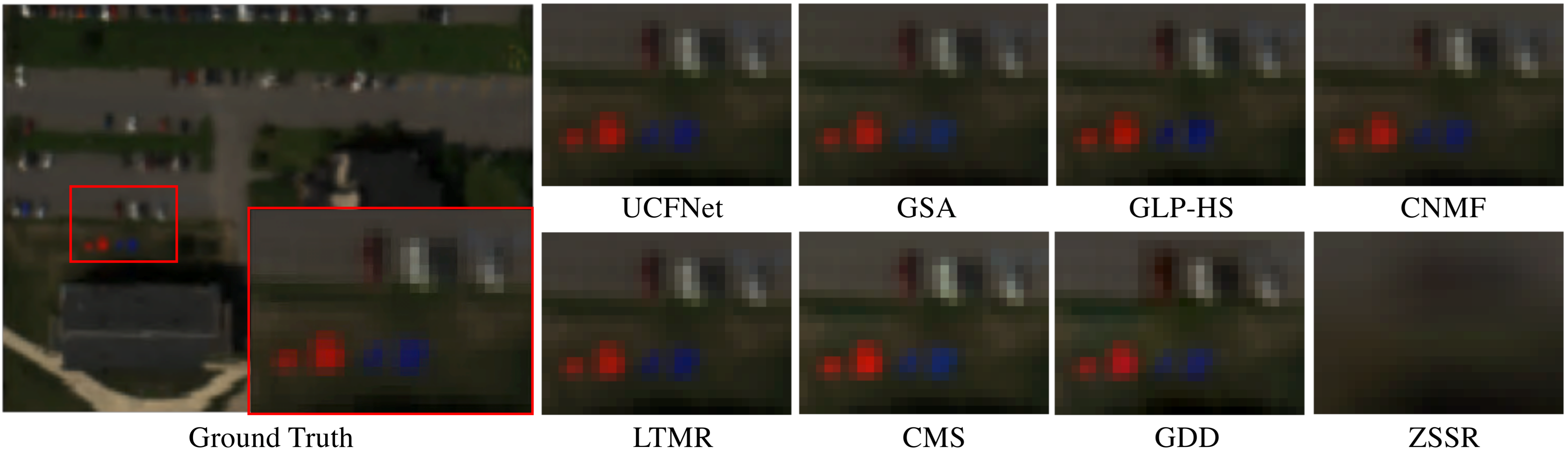
Dataset SHARE2010 [40] was collected by the ProSpecTIR-VS sensor over the city of Rochester, NY, USA, in July 2010. The sensor was configured to collect the radiance ranging from 390 to 2450 nm with a spectral resolution of 5 [nm]. Sites for data collection include the Genesee River, sections of downtown Rochester, and the Rochester Institute of Technology (RIT) campus, and the ROI we selected in this paper is a 120 × 160 region of RIT.

4.2. Evaluation Criterion

Three quantitative metrics are used to evaluate the quality of the reconstructed full-spectrum HR-HSI, including peak signal-to-noise ratio (PSNR), the structural similarity (SSIM) [42], and Spectral Angle Mapper (SAM) [38]. Among these metrics, the average PSNR and SSIM of all bands in the reconstructed hyperspectral images are reported. The higher averaged PSNR/SSIM value, the better. Meanwhile, the averaged SAM of all pixels is used to evaluate the global spectral accuracy. The visualization of SAM is used to assess the per-pixel spectral reconstruction performance. The lower SAM value indicates better spectral accuracy. Additionally, to focus on the application-oriented accuracy issues, a classification algorithm is employed. The closest test accuracy of reconstructed HR-HSI to that of the round-truth image indicates the best per-pixel spectral accuracy achieved by the corresponding sharpening method.

We adopt per-pixel classification here as a measurement of the per-pixel accuracy from an application perspective. Since the class map of dataset AVIRIS-NG-Cuprite is unavailable, we use the MaxD and Gram matrix algorithms [43,44] to extract distinct materials (called endmembers) and then use SAM to create the ground truth training data for the support vector machine classifier. The detailed steps are: First, the MaxD and Gram matrix algorithms are implemented to extract endmembers from the ground-truth HR-HSI. Second, we generate the classification map by individual thresholding the spectral angle between each pixel and each endmember. That is, the pixel is labeled as the class number of the endmember giving the smallest spectral angle. If none of the spectral angle errors between each endmember are below a small threshold (such as 0.1 radians), then the pixel is un-labeled. Third, 70 percent of the labeled pixels are used for the linear Support Vector Classification (SVC) [45] training, and the rest of the 30 percent of data are used for testing. When the test accuracy is approaching 100 percent, we call the classifier well-trained. Then, the trained SVC is applied to different generated HR-HSIs. By comparing the accuracy and confusion matrix, we can tell which image has the best radiometric accuracy as measured in the application of classification. Our goal is to find the sharpened result which has the closest test accuracy to the ground truth data, which demonstrates the corresponding sharpening method has the capability to generate the image with the highest per-pixel spectral accuracy.

4.3. Experiment Setup

Our UCFNet is trained with 50,000 epochs. ADAM optimizer [46] is used to optimize the network parameters, the learning rate is $7\times {10}^{-3}$. Moreover, the weights $\mu$ and $\lambda$ of the loss function shown in Equation (5) are set to 1 and $1\times {10}^{-2}$, respectively. The experiments of the conventional methods were implemented in MATLAB R2020b on macOS with an Intel Core i7 2.2GHz CPU. The learning-based methods are performed in Pytorch with a Tesla P100 GPU.

4.4. Results

(1) Dataset AVIRIS-NG-Cuprite:

Table 1. Quantitative performance comparison of different algorithms on dataset AVIRIS-NG-Cuprite. The up-arrow means the higher the value, the better the performance. The down-arrow means the lower the value, the better the performance. S denotes the value of the up-scale factor. The best performances are highlighted in bold.

S		UCFNet	GSA	GLP-HS	CNMF	CMS	LTMR	GDD	ZSSR
2	Mean SAM ↓	0.0084	0.0091	0.0120	0.0093	0.0204	0.0118	0.0101	0.0102
	Mean SSIM ↑	0.9962	0.9944	0.9920	0.9948	0.9458	0.9931	0.9949	0.9734
	Mean PSNR ↑	49.0772	47.2153	45.3593	49.0620	36.6297	47.2524	47.7830	38.6947
4	Mean SAM ↓	0.0109	0.0134	0.0158	0.0130	0.0192	0.0163	0.0180	0.0153
	Mean SSIM ↑	0.9924	0.9874	0.9831	0.9871	0.9556	0.9843	0.9758	0.9281
	Mean PSNR ↑	47.0997	43.9079	42.8805	43.2027	38.1846	45.0513	39.8599	34.1080
8	Mean SAM ↓	0.0141	0.0180	0.0208	0.0174	0.0248	0.0271	0.0303	0.0225
	Mean SSIM ↑	0.9872	0.9799	0.9737	0.9774	0.9387	0.9581	0.9481	0.8819
	Mean PSNR ↑	44.6770	41.5907	40.6665	39.4293	37.1484	41.5918	34.4552	30.9458

summarizes the averaged SAM, PSNR and SSIM of the compared approaches. From this table, we can see that the proposed UCFNet has the best performance across all scale factors. It is worth noticing that, as the up-scale ratio goes up, rapid performance degradations are measured for GSA, GLP-HS, GDD and ZSSR, which reveals the ineffectiveness of these approaches in the challenging scenarios. The color composites of the obtained outcomes are displayed in Figure 4. It can be seen that no obvious spatial distortions are observed in the testing approaches, except ZSSR. However, according to the spectral angle maps shown in Figure 5, UCFNet has the smallest spectral errors, while other competitors have worse performance.

In order to demonstrate the spectral quality of the sharpened images, we plot some spectral reflectance difference curves (up-scale factor = 8) in Figure 6. Similar to the method of creating the class map introduced in Section 4.2, the target map of four different materials is obtained by strictly thresholding the SAMs between the reference HR-HSI and each endmember. Then, the locations of these materials on the generated HR-HSI can be easily found based on the target map. Finally, the spectrum difference is calculated between the averaged target pixels in the reference HR-HSI and that in the reconstructed HR-HSI. Figure 6 illustrates that, for both VNIR and SWIR bands, our UCFNet has the best spectral patterns approximation to the ground truth. CMS, GDD and ZSSR fail in spectral reconstruction among the whole spectrum, while GSA, GLP-HS, CNMF, and LTMR have better spectral reconstruction on Vis-NIR bands, but high spectral distortion on the SWIR bands.

Lastly, the linear Support Vector Classification (SVC) is implemented to evaluate how the per-pixel accuracy impacts classification results. Due to the fact that a class map of the AVIRIS-NG-Cuprite dataset is unavailable, we created the class map based on the method introduced in Section 4.2, which is shown in Figure 7. Label 0 represents all of the un-labeled pixels and labels 1 to 11 represent the class endmember 1 to endmember 11. Next, 70 percent per-class of the labeled pixels are used for the linear SVC training, and the rest of the data forms the test set. Once the accuracy is approaching 100 percent, we call the classifier well-trained. Then, the trained SVC classifier is applied to the generated HR-HSI delivered by the different testing methods. Both overall accuracy and averaged per-class accuracy are listed in

Table 2. Test accuracy of classification results of the compared approaches. The scaling factor is 8. The best performances are highlighted in bold.

Methods	Reference	UCFNet	GSA	CNMF	GLP-HS	LTMR	CMS	GDD	ZSSR
Overall Accuracy (%)	99.61	90.11	86.88	84.20	87.48	79.60	82.52	80.79	81.83
Averaged Per-class Accuracy (%)	98.39	80.23	70.54	62.51	76.77	70.08	63.42	70.95	66.61

. This shows that UCFNet outperforms competitors, which means that the HR-HSI generated by UCFNet has the best per-pixel radiometric accuracy when assessed for the task of classification. For CNMF, CMS and ZSSR, their per-class accuracy is significantly lower than the overall accuracy, which indicates they are ineffective in recovering accurate spectra of rare-distributed materials. Furthermore, the confusion matrices of three methods, that have top-ranked classification accuracy, are presented in Figure 8 allowing us to observe the classification and mis-classification status for each individual endmember. Our method performs well on spectra reconstruction for endmembers 2, 3, 6, and 10. However, endmember 1 and 5, endmember 1 and 9, and endmember 7 and 9 have high percentages being wrongly classified, which may result from the fact that these endmembers have high spectral-similarity between each other. Meanwhile, GSA and GLP-HS have more mis-classifiions compared to UCFNet. For instance, they have higher mis-classified pixels between endmember 2 and 5, endmember 5 and 7, and endmember 9 and 10, which further supports the advantage of the proposed approach.

(2) Dataset SHARE-2010:

Table 3. Quantitative performance comparison of different algorithms on dataset SHARE-2010. The up-arrow means the higher the value, the better the performance. The down-arrow means the lower the value, the better the performance. The best performances are highlighted in bold. S represents the value of up-scale ratio.

S		UCFNet	GSA	CNMF	GLP-HS	LTMR	CMS	GDD	ZSSR
2	Mean SAM ↓	0.0197	0.0282	0.0295	0.0292	0.0300	0.0703	0.0226	0.0404
	Mean SSIM ↑	0.9979	0.9960	0.9964	0.9969	0.9968	0.9729	0.9967	0.9681
	Mean PSNR ↑	49.7991	46.1933	46.9932	49.9470	49.2730	38.8847	49.7782	40.6667
4	Mean SAM ↓	0.0240	0.0468	0.0375	0.0420	0.0401	0.0773	0.0519	0.0628
	Mean SSIM ↑	0.9965	0.9889	0.9923	0.9905	0.9938	0.9637	0.9845	0.9138
	Mean PSNR ↑	48.5506	41.9736	44.3017	42.3004	47.2764	38.2235	41.2772	30.3932
8	Mean SAM ↓	0.0348	0.0735	0.0478	0.0537	0.0596	0.0981	0.0672	0.0961
	Mean SSIM ↑	0.9923	0.9805	0.9876	0.9764	0.9767	0.9392	0.9815	0.8040
	Mean PSNR ↑	43.1981	38.0056	42.0831	36.4299	44.4230	35.0870	39.6866	25.9654

shows the quantitative performance comparison between different methods, clearly reveals that our UCFNet has the most stable and best performance. Moreover, the RGB images of the sharpened results and the spectral angle maps are displayed in Figure 9. It shows that all the compared methods provide good qualitative results, except ZSSR. However, in Figure 10, the SAMs shows that GSA and GDD have serious spectral distortions in the shadows. CMS and ZSSR have high spectral errors happen on the edges and shadows as well. The darkest SAM of UCFNet indicates the best spectral information reconstruction.

4.5. Discussion

The proposed UCFNet outperforms the compared approaches because the cascade training strategy is employed to gradually improve the spatial resolution of the image. Furthermore, the sharpened HR-HSI in the previous stage is used to calculate the loss between it and the degraded output in the next stage. In this way, the robustness of the proposed method is further improved. Furthermore, the proposed network uses the combined MSE and SAM as the total loss, which effectively improves the ability of UCFNet to better correct small errors during the training.

One common reason for the ineffectiveness of the compared methods is they are not specifically designed for sharpening the LR-HSI that covers Vis-NIR-SIWR bands. When the HR-MSI covers the Vis-NIR-SWIR bands, but the HR-MSI only covers the VNIR bands, the correlation between the LR-HSI and HR-MSI decreased dramatically. Moreover, the inconsistent edge distributions in the VNIR and SWIR bands of the hyperspectral data make the problem more challenging. Therefore, failing to consider these problems makes the baselines defeated by our UCFNet.

4.6. Ablation Study

In order to test how a change in the method of generating the preliminary HR-VNIR-HSI will impact the reconstructed results of UCFNet, experiments are conducted using GLP-HS and bilinear interpolation to separately generate preliminary HR-VNIR-HSI. From the quantitative results with dataset SHARE-2010 shown in

Table 4. The effect of using different up-sampling methods to initialize the preliminary HR-VNIR-HSI. The up-arrow means the higher the value, the better the performance. The down-arrow means the lower the value, the better the performance. The best performances are highlighted in bold.

	S	Mean SAM ↓	Mean PSNR ↑	Mean SSIM ↑
GLP-HS	4	0.0240	48.5506	0.9965
Bilinear	4	0.0243	48.1867	0.9929
GLP-HS	8	0.0348	43.1981	0.9923
Bilinear	8	0.0355	42.6240	0.9913

, we can see that using GLP-HS achieves better radiometric accuracy in the final results.

The main difference between using bilinear and GLP-HS for initializing the HR-VNIR-HSI is that bilinear upsampling is a simple mathematic interpolation algorithm that only utilizes the spatial information of the LR-HSI, while GLP-HS is designed for hyperspectral sharpening, which fully exploits the spectral and spatial correlations between HSI and MSI. Moreover, regarding conventional sharpening algorithms, the experiment results in work [35] show that GLP-HS has the most effective and stable performance with small spatial resolution ratios. Therefore, we chose GLP-HS to initialize the HR-VNIR-HSI in this paper.

5. Conclusions

We have presented a novel method, an unsupervised cascade fusion convolutional neural network (UCFNet), for Vis-NIR-SWIR hyperspectral sharpening. With the spectral information provided by the LR-HSI and the spatial details offered by the HR-MSI, our method is able to effectively improve the spatial resolution of the full-spectrum LR-HSI while maintaining high radiometric accuracy. Furthermore, to ensure a robust performance with large scaling ratios, we designed a cascade sharpening framework to progressively sharpen the image. Furthermore, the self-supervising loss is applied between the adjacent cascade stages, which further boosts the radiometric accuracy of the reconstructed image.

Seven baseline algorithms, GSA [3], GLP-HS [17], CNMF [6], LTMR [15], CMS [14], GDD [34], and ZSSR [22] are implemented. The AVIRIS-NG-Cuprite and SHARE-2010 Dataset are used for testing different approaches and different up-scale factors. According to the results of averaged SAM, PSNR, and SSIM, the proposed approach obtains a stable and high performance over the experiments presented. Furthermore, the reflectance difference plots show our UCFNet has the best performance on the reconstruction of the spectral details, especially on the SWIR part. Moreover, the test accuracy and the confusion matrix of classification result show the highest per-pixel spectral accuracy is achieved by the proposed method. All of the consistent results indicate a promising improvement of the performance of using the reconstructed HR-HSI for further spectral analysis.

References

1. Carper, W.; Lillesand, T.; Kiefer, R. The use of intensity-hue-saturation transformations for merging SPOT panchromatic and multispectral image data. Photogramm. Eng. Remote Sens. 1990, 56, 459–467. [Google Scholar]
2. Laben, C.A.; Brower, B.V. Process for Enhancing the Spatial Resolution of Multispectral Imagery Using Pan-Sharpening. U.S. Patent 6,011,875, 4 January 2000. [Google Scholar]
3. Aiazzi, B.; Baronti, S.; Selva, M. Improving component substitution pansharpening through multivariate regression of MS + Pan data. IEEE Trans. Geosci. Remote Sens. 2007, 45, 3230–3239. [Google Scholar] [CrossRef]
4. Liu, J. Smoothing filter-based intensity modulation: A spectral preserve image fusion technique for improving spatial details. Int. J. Remote Sens. 2000, 21, 3461–3472. [Google Scholar] [CrossRef]
5. Aiazzi, B.; Alparone, L.; Baronti, S.; Garzelli, A.; Selva, M. MTF-tailored multiscale fusion of high-resolution MS and Pan imagery. Photogramm. Eng. Remote Sens. 2006, 72, 591–596. [Google Scholar] [CrossRef]
6. Yokoya, N.; Yairi, T.; Iwasaki, A. Coupled nonnegative matrix factorization unmixing for hyperspectral and multispectral data fusion. IEEE Trans. Geosci. Remote Sens. 2011, 50, 528–537. [Google Scholar] [CrossRef]
7. Akhtar, N.; Shafait, F.; Mian, A. Sparse spatio-spectral representation for hyperspectral image super-resolution. In Proceedings of the European Conference on Computer Vision, Zurich, Switzerland, 6–12 September 2014; Springer: Cham, Switzerland, 2014; pp. 63–78. [Google Scholar]
8. Simoes, M.; Bioucas-Dias, J.; Almeida, L.B.; Chanussot, J. A convex formulation for hyperspectral image superresolution via subspace-based regularization. IEEE Trans. Geosci. Remote Sens. 2014, 53, 3373–3388. [Google Scholar] [CrossRef]
9. Lanaras, C.; Baltsavias, E.; Schindler, K. Hyperspectral super-resolution by coupled spectral unmixing. In Proceedings of the IEEE International Conference on Computer Vision, Santiago, Chile, 7–13 December 2015; pp. 3586–3594. [Google Scholar]
10. Wei, Q.; Dobigeon, N.; Tourneret, J.Y. Bayesian fusion of multi-band images. IEEE J. Sel. Top. Signal Process. 2015, 9, 1117–1127. [Google Scholar] [CrossRef]
11. Wei, Q.; Dobigeon, N.; Tourneret, J.Y. Fast fusion of multi-band images based on solving a Sylvester equation. IEEE Trans. Image Process. 2015, 24, 4109–4121. [Google Scholar] [CrossRef]
12. Akhtar, N.; Shafait, F.; Mian, A. Bayesian sparse representation for hyperspectral image super resolution. In Proceedings of the IEEE Conference on Computer Vision and Pattern Recognition, Boston, MA, USA, 7–12 June 2015; pp. 3631–3640. [Google Scholar]
13. Dian, R.; Fang, L.; Li, S. Hyperspectral image super-resolution via non-local sparse tensor factorization. In Proceedings of the IEEE Conference on Computer Vision and Pattern Recognition, Honolulu, HI, USA, 21–26 July 2017; pp. 5344–5353. [Google Scholar]
14. Zhang, L.; Wei, W.; Bai, C.; Gao, Y.; Zhang, Y. Exploiting clustering manifold structure for hyperspectral imagery super-resolution. IEEE Trans. Image Process. 2018, 27, 5969–5982. [Google Scholar] [CrossRef]
15. Dian, R.; Li, S. Hyperspectral image super-resolution via subspace-based low tensor multi-rank regularization. IEEE Trans. Image Process. 2019, 28, 5135–5146. [Google Scholar] [CrossRef]
16. Dian, R.; Li, S.; Kang, X. Regularizing hyperspectral and multispectral image fusion by CNN denoiser. IEEE Trans. Neural Netw. Learn. Syst. 2020, 32, 1124–1135. [Google Scholar] [CrossRef] [PubMed]
17. Selva, M.; Aiazzi, B.; Butera, F.; Chiarantini, L.; Baronti, S. Hyper-sharpening: A first approach on SIM-GA data. IEEE J. Sel. Top. Appl. Earth Obs. Remote Sens. 2015, 8, 3008–3024. [Google Scholar] [CrossRef]
18. Kwan, C.; Budavari, B.; Bovik, A.C.; Marchisio, G. Blind quality assessment of fused worldview-3 images by using the combinations of pansharpening and hypersharpening paradigms. IEEE Geosci. Remote Sens. Lett. 2017, 14, 1835–1839. [Google Scholar] [CrossRef]
19. Park, H.; Choi, J. A Comparison of Hyper-Sharpening Algorithms for Fusing VNIR and SWIR Bands of WorldView-3 Satellite Imagery. In Proceedings of the IGARSS 2018—2018 IEEE International Geoscience and Remote Sensing Symposium, Valencia, Spain, 22–27 July 2018; IEEE: Piscataway, NJ, USA, 2018; pp. 5124–5127. [Google Scholar]
20. Selva, M.; Santurri, L.; Baronti, S. Improving hypersharpening for WorldView-3 data. IEEE Geosci. Remote Sens. Lett. 2018, 16, 987–991. [Google Scholar] [CrossRef]
21. Ulyanov, D.; Vedaldi, A.; Lempitsky, V. Deep image prior. In Proceedings of the IEEE Conference on Computer Vision and Pattern Recognition, Salt Lake City, UT, USA, 18–22 June 2018; pp. 9446–9454. [Google Scholar]
22. Shocher, A.; Cohen, N.; Irani, M. “zero-shot” super-resolution using deep internal learning. In Proceedings of the IEEE Conference on Computer Vision and Pattern Recognition, Salt Lake City, UT, USA, 18–22 June 2018; pp. 3118–3126. [Google Scholar]
23. Haut, J.M.; Fernandez-Beltran, R.; Paoletti, M.E.; Plaza, J.; Plaza, A.; Pla, F. A new deep generative network for unsupervised remote sensing single-image super-resolution. IEEE Trans. Geosci. Remote Sens. 2018, 56, 6792–6810. [Google Scholar] [CrossRef]
24. Sidorov, O.; Yngve Hardeberg, J. Deep hyperspectral prior: Single-image denoising, inpainting, super-resolution. In Proceedings of the IEEE/CVF International Conference on Computer Vision Workshops, Seoul, Korea, 27–28 October 2019. [Google Scholar]
25. Jiang, J.; Sun, H.; Liu, X.; Ma, J. Learning spatial-spectral prior for super-resolution of hyperspectral imagery. IEEE Trans. Comput. Imaging 2020, 6, 1082–1096. [Google Scholar] [CrossRef]
26. Qu, Y.; Qi, H.; Kwan, C. Unsupervised sparse dirichlet-net for hyperspectral image super-resolution. In Proceedings of the IEEE Conference on Computer Vision and Pattern Recognition, Salt Lake City, UT, USA, 18–22 June 2018; pp. 2511–2520. [Google Scholar]
27. Nguyen, H.V.; Ulfarsson, M.O.; Sveinsson, J.R.; Sigurdsson, J. Zero-shot sentinel-2 sharpening using a symmetric skipped connection convolutional neural network. In Proceedings of the IGARSS 2020—2020 IEEE International Geoscience and Remote Sensing Symposium, Waikoloa, HI, USA, 26 September–2 October 2020; IEEE: Piscataway, NJ, USA, 2020; pp. 613–616. [Google Scholar]
28. Nguyen, H.V.; Ulfarsson, M.O.; Sveinsson, J.R.; Dalla Mura, M. Sentinel-2 Sharpening Using a Single Unsupervised Convolutional Neural Network With MTF-Based Degradation Model. IEEE J. Sel. Top. Appl. Earth Obs. Remote Sens. 2021, 14, 6882–6896. [Google Scholar] [CrossRef]
29. Salgueiro, L.; Marcello, J.; Vilaplana, V. Single-Image Super-Resolution of Sentinel-2 Low Resolution Bands with Residual Dense Convolutional Neural Networks. Remote Sens. 2021, 13, 5007. [Google Scholar] [CrossRef]
30. Lanaras, C.; Bioucas-Dias, J.; Baltsavias, E.; Schindler, K. Super-resolution of multispectral multiresolution images from a single sensor. In Proceedings of the IEEE Conference on Computer Vision and Pattern Recognition Workshops, Honolulu, HI, USA, 21–26 July 2017; pp. 20–28. [Google Scholar]
31. Lanaras, C.; Bioucas-Dias, J.; Galliani, S.; Baltsavias, E.; Schindler, K. Super-resolution of Sentinel-2 images: Learning a globally applicable deep neural network. ISPRS J. Photogramm. Remote Sens. 2018, 146, 305–319. [Google Scholar] [CrossRef]
32. Huang, Q.; Li, W.; Hu, T.; Tao, R. Hyperspectral image super-resolution using generative adversarial network and residual learning. In Proceedings of the ICASSP 2019—2019 IEEE International Conference on Acoustics, Speech and Signal Processing (ICASSP), Brighton, UK, 12–17 May 2019; IEEE: Piscataway, NJ, USA, 2019; pp. 3012–3016. [Google Scholar]
33. Shaham, T.R.; Dekel, T.; Michaeli, T. Singan: Learning a generative model from a single natural image. In Proceedings of the IEEE International Conference on Computer Vision, Seoul, Korea, 27–28 October 2019; pp. 4570–4580. [Google Scholar]
34. Uezato, T.; Hong, D.; Yokoya, N.; He, W. Guided deep decoder: Unsupervised image pair fusion. In Proceedings of the European Conference on Computer Vision, Glasgow, UK, 23–28 August 2020; Springer: Berlin/Heidelberg, Germany, 2020; pp. 87–102. [Google Scholar]
35. Huang, S.; Messinger, D.W. An Unsupervised Laplacian Pyramid Network for Radiometrically Accurate Data Fusion of Hyperspectral and Multispectral Imagery. IEEE Trans. Geosci. Remote Sens. 2022, 60, 5527517. [Google Scholar] [CrossRef]
36. Gargiulo, M.; Mazza, A.; Gaetano, R.; Ruello, G.; Scarpa, G. A CNN-based fusion method for super-resolution of Sentinel-2 data. In Proceedings of the IGARSS 2018—2018 IEEE International Geoscience and Remote Sensing Symposium, Valencia, Spain, 22–27 July 2018; IEEE: Piscataway, NJ, USA, 2018; pp. 4713–4716. [Google Scholar]
37. Pouliot, D.; Latifovic, R.; Pasher, J.; Duffe, J. Landsat super-resolution enhancement using convolution neural networks and Sentinel-2 for training. Remote Sens. 2018, 10, 394. [Google Scholar] [CrossRef] [Green Version]
38. Kruse, F.A.; Lefkoff, A.; Boardman, J.; Heidebrecht, K.; Shapiro, A.; Barloon, P.; Goetz, A. The spectral image processing system (SIPS)-interactive visualization and analysis of imaging spectrometer data. In AIP Conference Proceedings; American Institute of Physics: College Park, MD, USA, 1993; Volume 283, pp. 192–201. [Google Scholar]
39. The AVIRIS Next Generation Data.
40. Herweg, J.A.; Kerekes, J.P.; Weatherbee, O.; Messinger, D.; van Aardt, J.; Ientilucci, E.; Ninkov, Z.; Faulring, J.; Raqueño, N.; Meola, J. Spectir hyperspectral airborne rochester experiment data collection campaign. In Proceedings of the Algorithms and Technologies for Multispectral, Hyperspectral, and Ultraspectral Imagery XVIII, Baltimore, MD, USA, 23–27 April 2012; International Society for Optics and Photonics: Bellingham, WA, USA, 2012; Volume 8390, p. 839028. [Google Scholar]
41. Wald, L.; Ranchin, T.; Mangolini, M. Fusion of satellite images of different spatial resolutions: Assessing the quality of resulting images. Photogramm. Eng. Remote Sens. 1997, 63, 691–699. [Google Scholar]
42. Wang, Z.; Bovik, A.C.; Sheikh, H.R.; Simoncelli, E.P. Image quality assessment: From error visibility to structural similarity. IEEE Trans. Image Process. 2004, 13, 600–612. [Google Scholar] [CrossRef] [PubMed]
43. Canham, K.; Schlamm, A.; Ziemann, A.; Basener, B.; Messinger, D. Spatially adaptive hyperspectral unmixing. IEEE Trans. Geosci. Remote Sens. 2011, 49, 4248–4262. [Google Scholar] [CrossRef]
44. Messinger, D.W.; Ziemann, A.K.; Schlamm, A.; Basener, W. Metrics of spectral image complexity with application to large area search. Opt. Eng. 2012, 51, 036201. [Google Scholar] [CrossRef]
45. Gunn, S.R. Support Vector Machines for Classification and Regression; ISIS Technical Report; University of Southampton: Southampton, UK, 1998; Volume 14, pp. 5–16. [Google Scholar]
46. Kingma, D.P.; Ba, J. Adam: A method for stochastic optimization. arXiv 2014, arXiv:1412.6980. [Google Scholar]
Figure 1. The image fusion diagram of UCFNet.
Remotesensing 14 04390 g001
Figure 2. The architecture of the proposed generative network.
Remotesensing 14 04390 g002
Figure 3. The cascade sharpening strategy. Y is the LR-HSI and Y S is the VNIR part of Y . { X H R 1 , X H R 2 , X H R 3 } is the HR-MSI pyramid. { Z ˜ V 1 , Z ˜ V 2 , Z ˜ V 3 } are the preliminary HR-VNIR-HSIs. { Z ^ 1 , Z ^ 2 , Z ^ 3 } are the sharpened image at each stage. Z ^ S 1 and Z ^ S 2 are the SWIR parts of Z ^ 1 and Z ^ 2 . L s p e denotes the spectral loss, L s p e s e l f denotes the self-supervising loss, and L s p a denotes the spatial loss.
Remotesensing 14 04390 g003
Figure 4. Reconstructed composite images of the AVIRIS-NG-Cuprite dataset (R: 697 nm, G: 576 nm, B: 492 nm) with a scaling factor of 8.
Remotesensing 14 04390 g004
Figure 5. Error maps, AVIRIS-NG-Cuprite dataset, the scaling factor is 8.
Remotesensing 14 04390 g005
Figure 6. Spectral reflectance difference between of the reconstructed and the reference HSI. Dataset AVIRIS-NG-Cuprite with a scaling factor of 8. (a) Endmember 1. (b) Endmember 3. (c) Endmember 4. (d) Endmember 5.
Remotesensing 14 04390 g006
Figure 7. Left: The Cuprite ROI. Right: The class map.
Remotesensing 14 04390 g007
Figure 8. Confusion matrix of the linear SVM classifier. Left is the sharpened image of our method, middle is the sharpened image of GLP-HS, and right is the sharpened image of GSA.
Remotesensing 14 04390 g008
Figure 9. Reconstructed composite images of the SHARE-2010 dataset (R: 697 nm, G: 576 nm, B: 492 nm) with a up-scale factor of 8.
Remotesensing 14 04390 g009
Figure 10. Error maps, the SHARE-2010 dataset, the scaling factor is 8.
Remotesensing 14 04390 g010