Auto-Weighted Structured Graph-Based Regression Method for Heterogeneous Change Detection

Abstract

Change detection using heterogeneous remote sensing images is an increasingly interesting and very challenging topic. To make the heterogeneous images comparable, some graph-based methods have been proposed, which first construct a graph for the image to capture the structure information and then use the graph to obtain the structural changes between images. Nonetheless, previous graph-based change detection approaches are insufficient in representing and exploiting the image structure. To address these issues, in this paper, we propose an auto-weighted structured graph (AWSG)-based regression method for heterogeneous change detection, which mainly consists of two processes: learning the AWSG to capture the image structure and using the AWSG to perform structure regression to detect changes. In the graph learning process, a self-conducted weighting strategy is employed to make the graph more robust, and the local and global structure information are combined to make the graph more informative. In the structure regression process, we transform one image to the domain of the other image by using the learned AWSG, where the high-order neighbor information hidden in the graph is exploited to obtain a better regression image and change image. Experimental results and comparisons on four real datasets with seven state-of-the-art methods demonstrate the effectiveness of the proposed approach.

1. Introduction

1.1. Background

Change detection (CD) is a very important topic in remote sensing, which can detect changes occurring on the Earth’s surface by comparing images collected at different times [1]. CD has a wide range of applications, such as agricultural surveys, urban planning, environmental monitoring, and disaster assessment [2,3,4].

Previous CD methods often compare multitemporal images from the same sensor to extract changes, which can be referred to as homogeneous CD or monomodal CD, such as the homogeneous CD of SAR images [5], multispectral images [6,7], and hyperspectral images [8]. However, homogeneous CD has the limitation that the compared images from the same sensor may not always be acquired in time. In this case, we need to utilize the heterogeneous CD, i.e., using multitemporal images from different sensors to extract changes.

Heterogeneous CD can be regarded as an extension of homogeneous CD, which has two additional advantages (compared to homogeneous CD) [9,10]: first, it can reduce the response time of change analysis in emergency situations (such as floods, earthquakes, etc.) by using any available image independently of its modality, instead of having to wait for the homogeneous images to be sensed. More importantly, homogeneous images are often unavailable due to the accompanying adverse conditions of weather and lighting. Second, heterogenous CD can improve the temporal resolution of change analysis by inserting heterogeneous data.

1.2. Related Work

Compared to homogeneous CD, heterogeneous CD is more challenging because the multitemporal images are not directly comparable owing to the fact that they come from different modalities. In order to make heterogeneous images comparable, the first task addressed by heterogeneous CD is to transform them to the same domain, which is related to the topic of data transformation, feature learning, and domain adaptation [11,12,13].

As presented in [14,15,16], a more specific classification of heterogeneous CD methods is challenging. However, the distinction between using supervised data or not in the heterogeneous CD is still obvious. The supervised methods usually use the labeled unchanged data pairs to train the transformation functions [17,18,19]. However, acquiring supervised data is difficult in practice [20] as it requires high labor labeling costs and strong expert knowledge. To avoid the dependence on labeled data, unsupervised methods usually construct pseudo-training sets or use iterative methods to filter the training data [14,21,22,23]. At the same time, depending on the method used in the comparison, heterogeneous CD can also be divided into traditional machine learning-based and deep-learning-based. The former include methods using energy model [24], dictionary learning [25], copula theory [26], patch similarity graph [27,28], manifold learning [29], kernel canonical correlation analysis [30], fractal projection [15], graph learning [31], kernel regression [14,17]. The latter consist of methods using image style transferring network [32], cycle-consistent generative adversarial networks [18,33], commonality autoencoder [34], symmetric convolutional coupling network [22], self-supervised learning with Siamese networks [35,36].

Recently, a class of graph-based heterogeneous CD methods has been proposed, which usually first construct a graph for each image to capture the structure information, and then operate on the graphs to obtain changes. Specifically, Wu et al. [37] propose a semi-supervised multiscale graph convolutional network (GCN) to treat the CD problem as a node classification task, which constructs a multiscale graph for the stacked image and then propagates the information from labeled nodes to unlabeled ones by using GCN. The graph fusion-based CD method (GFBCD) [38] first constructs an approximate local graph for each image by using the Nystrom extension, and then fuses the graphs to calculate the changes by minimizing similarity between graphs. Furthermore, the GFBCD is improved in [39] by using a signal smoothness representation in the graph learning stage and a graph Laplacian-based regularization in the change estimating stage, which is referred to as GSMO-CD for short.

Based on the structure consistency between heterogeneous images, two types of graph-based methods are proposed: structure comparison methods and structure regression methods. For the former, they first construct a k-nearest-neighbors (KNN) graph for each image with Euclidean distance metric, and then directly compare the differences between the graphs by graph projection, such as the nonlocal patch similarity graph-based method (NPSG) [40], the improved nonlocal patch graph-based method (INLPG) [28], the iterative robust graph and Markovian co-segmentation-based method (IRG-McS) [23]. For the structure regression-based methods, a graph is first constructed for the pre-event image, and then the pre-event image is translated to the domain of post-event image by a structural regression or projection model, and finally, the translated image and post-event image are compared in the same domain as the homogeneous CD problem, such as the sparse-constrained adaptive structure consistency-based method (SCASC) [10], the fractal projection and Markovian segmentation method (FPMS) [15], and the adaptive graph with structure cycle consistency-based method (AGSCC) [9]. In addition, both types of the structure comparison methods and structure regression methods can be incorporated into the framework of graph signal processing for heterogeneous change detection (HCD-GSP): the structure comparison methods can be regarded as computing the difference of the same graph signal passing through different graphs in the vertex domain filtering of HCD-GSP [41], while the structure regression methods can be regarded as computing the difference of different graph signals passing through the same graph filter with the spectral domain analysis of HCD-GSP [42].

For these graph-based heterogeneous CD methods [9,10,15,23,28,37,38,39,40], there are three attractive advantages: first, they focus on structural features rather than illumination features (or pixel-wise features), which are very robust under different imaging conditions, while also being able to mitigate the effects of noise; second, they extract changes by analyzing the graph vertices, whose number is much smaller than the number of pixels, thus significantly reducing the complexity of operations; third, these methods are all very intuitive and interpretable (with clear physical meaning), while being able to be combined with other frameworks and extended to other applications.

1.3. Motivation and Contribution

Motivated by recent advances of the graph-based HCD methods, this paper proposes an auto-weighted structured graph (AWSG)-based method, which falls under the structure regression-based approach described above. Compared with the structure comparison methods that only provide the change results, i.e., difference image (DI) or the change map (CM), the structure regression methods also provide a translated image of another moment, which has a stronger visualization effect.

For the graph-based heterogeneous CD methods, two main aspects need to be solved: first, how to construct the graph to represent the image structure; second, how to detect changes by using the graph. Although the previous methods have achieved relatively promising results, they still have limitations in the above two aspects.

(1) First, the graph constructed by the previous method is not robust enough. The KNN graph is the most widely used to capture the structure information, such as INLPG [28], GSMO-CD [39], IRG-McS [23], SCASC [10], AGSCC [9]. It is well known that the KNN graph faces two challenges: the number (k) of nearest neighbors (NNs) and the distance metric. INLPG and GSMO-CD connect each vertex to its NNs with a fixed number of edges (k) without considering the proportion of objects represented by each vertex, which will under-connect the vertex with many truly similar vertices and over-connect the vertex with few truly similar vertices, thus making the graph unstable. To address this challenge, SCASC, IRG-McS, and AGSCC use an in-degree-based strategy to select an adaptive k for each vertex. However, the previous methods directly use the Euclidean distance metric and ignore the feature difference in the graph construction or graph learning, that is, these methods calculate the distance or similarity between vertices by assigning the same weight to all features while ignoring the distinguishing capability of different features in heterogeneous images.

In this paper, we learn an adaptive KNN graph for the structure regression method, which can connect each vertex to suitable similar neighbors with appropriate weights by using two techniques. First, it uses the k selection strategy proposed in IRG-McS [23] to choose the number of NNs for each vertex. Second, but more importantly, it uses an auto-weighted distance metric that adaptively assigns different weights for different features by using a self-conducted weight learning, which can make the graph more robust.

(2) Second, the graphs constructed by the previous methods cannot completely characterize the structure of the image, i.e., the representation ability of these graphs is insufficient. For example, the FPMS [15] and PSGM [27] use the self-expression property to learn the graph that can reconstruct each vertex by using other connected vertices, which can capture the global structure of an image. The SCASC [10] and INLPG [28] use the self-similarity property to construct the graph that connects each vertex with its NNs, which can capture the local structure of an image. However, from the perspective of information mining, we certainly hope that the graph can characterize richer structural information, which is more conducive to the subsequent structure comparison or structure regression for heterogeneous CD.

In this paper, we combine the local and global structure information to learn a structured graph, which uses the self-expression property to preserve the global structure of an image and uses the adaptive neighbor approach to capture the local structure of an image. In the graph learning process, we incorporate the local similarity-based regularization and global self-expression-based regularization. Then, the structured graph can find the most informative neighbors for each target vertex, which are not only the NNs of this target node, but can also reconstruct this target node using the corresponding edge weights. Therefore, the proposed graph can contain more structure information than graphs providing only global structure information [15] and graphs providing only local structure information [10].

(3) Third, previous methods have not fully utilized the information contained in the graph to detect changes. Once the graphs are constructed or learned, they are directly fused as in GFBCD [38] and GSMO-CD [39], or compared by projection as in INLPG [28] and IRG-McS [23], or transformed for structure regression as in SCASC [10]. However, these methods only use the first-order neighborhood information of the graphs, that is, they only consider the connections between each vertex and its NNs that are directly adjacent to it, but ignore the high-order neighbor information hidden in the graph. Therefore, this insufficient exploitation of graph information limits the change detection performance.

Inspired by the GSP framework of the heterogeneous CD [41,42], we exploit the high-order neighbor information of the graph in the structure regression process, that is, the information (or attributes) of vertices that are within K-hop ($K\ge 2$) away from the target vertex are also propagate to this vertex. Specifically, in the structure regression model, we decompose the post-event image into the translated pre-event image and the change image, and constrain the translated image to inherit the structure of the pre-event image by incorporating the global self-expression constraint and local similarity constraint, which are derived from the high-order information of the graph learned from the pre-event image. By effectively exploiting the information contained in the graph, the proposed method can obtain a better regression image and change image, thus improving the CD performance.

The main contribution of this paper is to improve the performance of structure regression-based heterogeneous change detection methods from two aspects: structure representation and exploiting the graph information, which can be summarized as follows:

• We learn an auto-weighted structured graph to represent the image structure by using a self-conducted weight learning;
• We combine the local and global structure information in the graph learning process to obtain a more informative graph;
• We exploit the high-order neighbor information of the graph in the structure regression process;
• We conduct comprehensive experiments on different real datasets to demonstrate the effectiveness of the proposed method.

1.4. Outline

The remainder of this paper is composed of five sections. In Section 2, we describe the graph learning model. In Section 3, we describe the structure regression model. In Section 4, the experimental results are analyzed. Finally, Section 5 concludes this paper and discusses the future work.

2. Auto-Weighted Structured Graph Learning

We consider a pair of co-registered heterogeneous images of $\tilde{\mathbf{X}}\in {\mathbb{R}}^{I\times J\times C_x}$ and $\tilde{\mathbf{Y}}\in {\mathbb{R}}^{I\times J\times C_y}$ obtained by different sensors over the same region before and after a change event, respectively, where $C_x$ and $C_y$ represent the channel numbers of $\tilde{\mathbf{X}}$ and $\tilde{\mathbf{Y}}$, respectively. The goal of heterogeneous CD is to detect the changed region.

Since the heterogeneous images of $\tilde{\mathbf{X}}$ and $\tilde{\mathbf{Y}}$ are from different domains, we cannot directly compare them to calculate the change image. Therefore, we need to find the connection between them and make them comparable. As illustrated in [23], there is structural consistency between heterogenous images. We first segment $\tilde{\mathbf{X}}$ and $\tilde{\mathbf{Y}}$ into small parts (superpixels) of ${\tilde{\mathbf{X}}}_i$ and ${\tilde{\mathbf{Y}}}_i$, $i=1,\cdots ,N$, with the same segmentation map, then the structural consistency can be described in the following way: if ${\tilde{\mathbf{X}}}_i$ and ${\tilde{\mathbf{X}}}_j$ belong to the same type of object (behaving as they are quite similar), and none of them changed during the event, then ${\tilde{\mathbf{Y}}}_i$ and ${\tilde{\mathbf{Y}}}_j$ also belong to the same type of object (behaving as they are also quite similar). If we define the similarity relationships between the superpixels within the pre-event image, i.e., the relationships between ${\tilde{\mathbf{X}}}_i$ and ${\tilde{\mathbf{X}}}_j$, $i,j=1,\cdots ,N$, as the structure of pre-event image, then this structure can be inherited by the post-event image if no change occurs. Therefore, we can employ this structural consistency to perform the image translation, that is, transform the pre-event image to the domain of post-event image and then compare the translated image and post-event image in the same domain to obtain the change map. In this way, the proposed method contains four steps: (1) pre-processing; (2) learning graph to capture the image structure; (3) translating image by using structural consistency; (4) extracting changes by binary segmentation. The framework of the proposed method is shown in Figure 1.

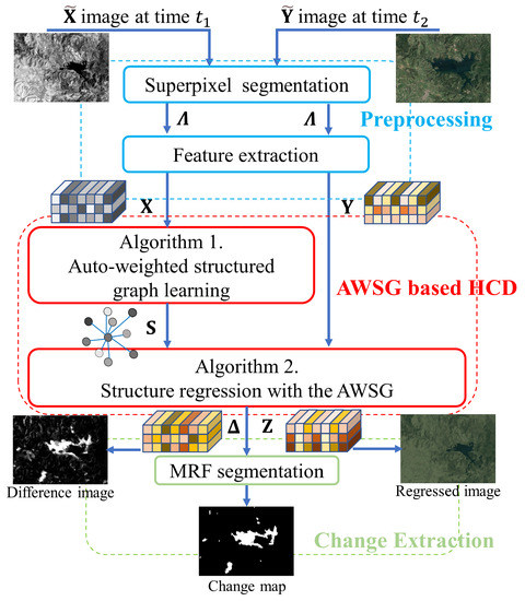
Figure 1. Framework of the proposed AWSG-based HCD method.

2.1. Pre-Processing

As the pairwise relationships is used to represent the image structure, we choose the superpixel as the basic processing unit, which has two advantages: first, it can contain sufficient contextual information and preserve the edges of the object; second, it can greatly reduce the computational complexity of the proposed method.

We choose the fractal net evolution approach (FNEA) [43] to complete the superpixel segmentation because of its good performance on both efficiency and boundary preservation. We first stack the pre-event image and post-event image into a stacked image with $C_x+C_y$ channels, then we use the FNEA to segment this stacked image into N superpixels with the segmentation map $\Lambda$. Then, we project this segmentation map to the original images to obtain the superpixels of ${\tilde{\mathbf{X}}}_i$ and ${\tilde{\mathbf{Y}}}_i$, $i=1,\cdots ,N$, so that the pair of superpixels with the same index from different image (such as ${\tilde{\mathbf{X}}}_i$ and ${\tilde{\mathbf{Y}}}_i$) represent the same spatial region.

After obtaining the superpixels, different features can be extracted, such as the spectral, spatial, and textural features. For each channel of the i-th superpixel, we extract M features and define the m-th feature extraction operator as ${\mathcal{F}}^{\left(m\right)}$, then we can obtain the feature vectors as ${\mathbf{X}}_i^m={\mathcal{F}}^{\left(m\right)}\left({\tilde{\mathbf{X}}}_i\right)\in {\mathbb{R}}^{C_x}$ and ${\mathbf{Y}}_i^m={\mathcal{F}}^{\left(m\right)}\left({\tilde{\mathbf{Y}}}_i\right)\in {\mathbb{R}}^{C_y}$. Then, we can obtain the stacked feature matrices as $\mathbf{X}\in {\mathbb{R}}^{C_x\times N\times M}$ and $\mathbf{Y}\in {\mathbb{R}}^{C_y\times N\times M}$, where ${\mathbf{X}}^m={\mathbf{X}}_{:,:,m}\in {\mathbb{R}}^{C_x\times N}$ and ${\mathbf{Y}}^m={\mathbf{Y}}_{:,:,m}\in {\mathbb{R}}^{C_y\times N}$ represents the m-th feature matrices.

2.2. Graph Learning

To capture the structure information of the pre-event image, we construct a directed weighted graph $\mathbf{G}=\left(V,E,S\right)$, where the vertex set is $V=\left\{{\tilde{\mathbf{X}}}_1,{\tilde{\mathbf{X}}}_2,\cdots ,{\tilde{\mathbf{X}}}_N\right\}$ that sets each superpixel as a vertex, and the edge set is $E=\left\{\left({\tilde{\mathbf{X}}}_i,{\tilde{\mathbf{X}}}_j\right)|S_{i,j}\ne 0;i,j=1,\cdots ,N\right\}$ that connects ${\tilde{\mathbf{X}}}_i$ to ${\tilde{\mathbf{X}}}_j$ with the weight $S_{i,j}$.

2.3. Structured Graph Learning Model

In SCASC [10], a distance-induced graph is proposed, which is based the intuitive constraint: the smaller the distance between ${\tilde{\mathbf{X}}}_i$ and ${\tilde{\mathbf{X}}}_j$, the larger the weight between them, i.e., $S_{i,j}$, should be. SCASC learns the local structure with the following model:

$$\underset{\mathbf{S}}{min}\sum _{i,j=1}^N{d}_{i,j}^x{S}_{i,j}+\alpha {\left(S_{i,j}\right)}^2,s.t.\sum _{i=1}^N{S}_{i,j}=1,S_{i,j}\ge 0$$

(1)

where $d_{i,j}^x$ is the distance between superpixels of ${\tilde{\mathbf{X}}}_i$ and ${\tilde{\mathbf{X}}}_j$ and $\alpha >0$ is a penalty parameter. As will be shown latter, the $\mathbf{S}$ is a sparse column when choosing a suitable $\alpha$. This type of graph describes the similarity relationships between each vertex and its local nearest neighbors.

Different from SCASC, the self-expression property is applied to learn the global structure in PSGM [27], which assumes that each vertex can be reconstructed by other connected vertices. PSGM learns the graph by using the following model:

$$\begin{array}{c}\hfill \underset{\mathbf{S}}{min}f\left(\mathbf{S}\right),s.t.{\mathbf{X}}^m={\mathbf{X}}^m\mathbf{S},S_{i,j}\ge 0\end{array}$$

(2)

where $f\left(\mathbf{S}\right)$ is the regularization of $\mathbf{S}$. As (2) uses all the vertices to represent each vertex with the self-weighing matrix as ${\mathbf{X}}_i^m={\mathbf{X}}^m{\mathbf{S}}_i$, this graph is expected to contain global structure information of the pre-event image.

As has been shown in many problems, such as classification [44], clustering [45,46], and feature selection [47], both global and local structural information are essential for graph performance because they can provide complementary information. In this paper, we combine the local structure learning of (1) and global structural learning of (2) into a structured graph learning model as

$$\begin{array}{c}\hfill \underset{\mathbf{S},\epsilon }{min}\sum _{i,j=1}^N{d}_{i,j}^x{S}_{i,j}^{}+\alpha {\left(S_{i,j}^{}\right)}^2+\beta \sum _{m=1}^{M}g\left({\epsilon }^m\right)\\ \hfill s.t.{\mathbf{X}}^m={\mathbf{X}}^m\mathbf{S}+{\epsilon }^m,\sum _{i=1}^N{S}_{i,j}=1,S_{i,j}\ge 0\end{array}$$

(3)

where $\beta >0$ represents tuning parameters, $\epsilon$ denotes the self-expression error caused by the noise or corruption, $g\left(·\right)$ denotes the penalty term. In the model (3), the local structure penalty term of ${\sum }_{i,j=1}^N{d}_{i,j}^x{S}_{i,j}^{}$ tends to provide a smaller weight $S_{i,j}$ to the edge $\left({\tilde{\mathbf{X}}}_i,{\tilde{\mathbf{X}}}_j\right)$ when the distance between ${\tilde{\mathbf{X}}}_i$ and ${\tilde{\mathbf{X}}}_j$ is larger. The global self-expression penalty term of ${\sum }_{m=1}^{M}g\left({\epsilon }^m\right)$ tends to reconstruct ${\mathbf{X}}_i$ from the whole $\mathbf{X}$ with ${\mathbf{S}}_i$ as ${\mathbf{X}}_i^m\approx {\sum }_{j=1}^N{\mathbf{X}}_j^m{S}_{j,i}$. The smooth regularizer of ${\sum }_{i,j=1}^N\alpha {\left(S_{i,j}^{}\right)}^2$ is used to avoid a trivial solution and make $\mathbf{S}$ column-sparse with the constraint of ${\sum }_{i=1}^N{S}_{i,j}=1,S_{i,j}\ge 0$. Specially, if we choose $\alpha =0$, we have a trivial solution for ${\mathbf{S}}_i$ as $S_{i,i}=1$ and $S_{j,i}=0$, $j\ne i$; if we set $\alpha \to \infty$, we have the trivial solution for ${\mathbf{S}}_i$ as ${\mathbf{S}}_i={\mathbf{1}}_N/N$, where ${\mathbf{1}}_N$ denotes an $N\times 1$ column vector of ones.

2.4. Weighted Graph Learning Model

In the structured graph learning model of (3), there are two points that directly affect the performance of the graph: the $\alpha$ that determines the number of NNs, and the distance metric that determines the neighbors position and weight of $\mathbf{S}$. That is, $\alpha$ controls the number of non-zero elements in $\mathbf{S}$, and $d_{i,j}^x$ and $g\left({\epsilon }^m\right)$ controls the index and value of each non-zero element of $\mathbf{S}$.

The previous methods usually connect each vertex to its NNs with a fixed number of edges (k) without considering the proportion of objects, such as INLPG [28], NPSG [40], GSMO-CD [39], which will cause under-connection or over-connection of some vertices. Meanwhile, the previous methods directly use the Euclidean distance metric and ignore the distinguishing capability of different features in heterogeneous images in the graph learning, such as SCASC [10], INLPG [28], IRG-McS [23], which is not robust and limits the structural representational capacity of the graph. To address these two problems, a weighted structured graph learning model can be used

$$\begin{array}{cc}\hfill \underset{\mathbf{S},\epsilon ,w}{min}& \sum _{m=1}^M{w}_m\left\{\sum _{i,j=1}^N{d}_{i,j,m}^x{S}_{i,j}+\beta g\left({\epsilon }^m\right)\right\}+\sum _{i=1}^N{\alpha }_i{∥{\mathbf{S}}_i∥}_2^2\hfill \\ \hfill & s.t.{\mathbf{X}}^m={\mathbf{X}}^m\mathbf{S}+{\epsilon }^m,\sum _{i=1}^N{S}_{i,j}=1,S_{i,j}\ge 0,\sum _{m=1}^M{w}_m^{\eta }=1,w_m\ge 0\hfill \end{array}$$

(4)

where $d_{i,j,m}^x={∥{\mathbf{X}}_i^m-{\mathbf{X}}_j^m∥}_2^2$ denotes the m-th feature distance between ${\tilde{\mathbf{X}}}_i$ and ${\tilde{\mathbf{X}}}_j$, $w_m$ denotes the m-th feature weight, and ${\alpha }_i>0$ is used to determine the NNs number of the i-th vertex, and $\eta >0$ is used to control the weights distribution. By comparing the models (3) and (4), we find that the weighted structured graph learning model (4) employs the parameter ${\alpha }_i$ for each vertex to control the number of NNs, and introduces the $w_m$ to assign the weights for different features.

2.5. Auto-Weighted Structured Graph Learning

As we know, the fewer the parameters to be adjusted, the more robust the graph learning model. We can find that $\eta$ can be adjusted in a larger range and $\eta$ is crucial to the performance of graph learning in (4). Additionally, we want to eliminate the need for manual adjustment of this parameter for different images, that is, we expect to remove such a parameter while pursuing good learning performance.

Motivated by recently proposed iteratively re-weighted technique [48], we propose an auto-weighted structured graph learning model by using a self-conducted weight learning

$$\begin{array}{c}\hfill \underset{\mathbf{S},\epsilon }{min}\sum _{m=1}^M\sqrt{\sum _{i,j=1}^N{d}_{i,j,m}^x{S}_{i,j}^{}+\beta g\left({\epsilon }^m\right)}+\sum _{i=1}^N{\alpha }_i{∥{\mathbf{S}}_i∥}_2^2\\ \hfill s.t.{\mathbf{X}}^m={\mathbf{X}}^m\mathbf{S}+{\epsilon }^m,\sum _{i=1}^N{S}_{i,j}=1,S_{i,j}\ge 0\end{array}$$

(5)

We can find that no weight factors are explicitly defined in (5). The Lagrange function of the minimization problem (5) can be formulated as

$$\begin{array}{c}\hfill \mathcal{L}\left(\mathbf{S},\epsilon ,\Psi \right)=\sum _{m=1}^M\sqrt{\sum _{i,j=1}^N{d}_{i,j,m}^x{S}_{i,j}^{}+\beta g\left({\epsilon }^m\right)}+\sum _{i=1}^N{\alpha }_i{∥{\mathbf{S}}_i∥}_2^2+\mathcal{G}\left(\Psi ,S,\epsilon \right)\end{array}$$

(6)

where $\mathcal{G}\left(\Psi ,S,\epsilon \right)$ is the formalized term derived from the constraints of (5) with $\Psi$ representing the Lagrange multipliers. Taking the derivative of (6) with respect to $\mathbf{S}$ and $\epsilon$, and setting them to zero, we can obtain   

$$\begin{array}{c}\hfill \sum _{m=1}^M{w}_m\frac{\partial \sum _{i,j=1}^N{d}_{i,j,m}^x{S}_{i,j}+\beta g\left({\epsilon }^m\right)}{\partial \mathbf{S}}+\frac{\partial \mathcal{G}\left(\Psi ,S,\epsilon \right)}{\partial \mathbf{S}}=0;\\ \hfill \sum _{m=1}^M{w}_m\frac{\partial \sum _{i,j=1}^N{d}_{i,j,m}^x{S}_{i,j}+\beta g\left({\epsilon }^m\right)}{\partial {\epsilon }^m}+\frac{\partial \mathcal{G}\left(\Psi ,S,\epsilon \right)}{\partial {\epsilon }^m}=0\end{array}$$

(7)

where

$$\begin{array}{c}\hfill w_m=\frac{1}{2\sqrt{\sum _{i,j=1}^N{d}_{i,j,m}^x{S}_{i,j}+\beta g\left({\epsilon }^m\right)}}\end{array}$$

(8)

Note that $w_m$ is determined by the target variables of $\mathbf{S}$ and $\epsilon$, so (5) cannot be directly solved. However, if $w_m$ is set to be satisfactory, (5) can be regarded as the solution of the problem

$$\begin{array}{cc}\hfill \underset{\mathbf{S},\epsilon }{min}& \sum _{m=1}^M{w}_m\left\{\sum _{i,j=1}^N{d}_{i,j,m}^x{S}_{i,j}+\beta g\left({\epsilon }^m\right)\right\}+\sum _{i=1}^N{\alpha }_i{∥{\mathbf{S}}_i∥}_2^2\hfill \\ \hfill & s.t.{\mathbf{X}}^m={\mathbf{X}}^m\mathbf{S}+{\epsilon }^m,\sum _{i=1}^N{S}_{i,j}=1,S_{i,j}\ge 0,\hfill \end{array}$$

(9)

which can be solved. This inspires us to use an iterative method to optimize problem (5): updating $\mathbf{S}$ by solving problem (9) with fixed $w_m$, and then updating $w_m$ by using (8) with fixed $\mathbf{S}$ and $\epsilon$.

2.6. Optimization

Define the m-th feature distance matrix as ${\mathbf{D}}_x^m$, whose $i,j$-th element is $d_{i,j,m}^x$, i.e., the m-th feature distance between superpixels ${\tilde{\mathbf{X}}}_i$ and ${\tilde{\mathbf{X}}}_j$, and  define ${\alpha }^{\frac{1}{2}}$ as a diagonal matrix with the i-th diagonal element being $\sqrt{{\alpha }_i}$. Then, we can rewrite the problem (9) as

$$\begin{array}{cc}\hfill \underset{\mathbf{S},\epsilon }{min}& \sum _{m=1}^M{w}_m\left\{Tr\left({\mathbf{S}}^T{\mathbf{D}}_x^m\right)+\beta g\left({\epsilon }^m\right)\right\}+{∥\mathbf{S}{\alpha }^{\frac{1}{2}}∥}_F^2\hfill \\ \hfill & s.t.{\mathbf{X}}^m={\mathbf{X}}^m\mathbf{S}+{\epsilon }^m,{\mathbf{S}}^T{\mathbf{1}}_N={\mathbf{1}}_N,\mathbf{S}\ge 0\hfill \end{array}$$

(10)

where $Tr\left(·\right)$ represents the matrix trace.

Next, we use the alternating direction method of multipliers (ADMM) to solve the minimization problem of (10). First, we introduce an auxiliary variable $\mathbf{P}\in {\mathbb{R}}^{N\times N}$, and rewrite the model (9) as the minimization of

$$\begin{array}{cc}\hfill \mathcal{L}\left(\mathbf{S},\epsilon ,\mathbf{P}\right)=& \sum _{m=1}^M{w}_m\left\{Tr\left({\mathbf{S}}^T{\mathbf{D}}_x^m\right)+\beta g\left({\epsilon }^m\right)\right\}+{∥\mathbf{S}{\alpha }^{\frac{1}{2}}∥}_F^2\hfill \\ \hfill & +Tr\left({\left(\mathbf{S}-\mathbf{P}\right)}^T{\mathbf{R}}_1\right)+\sum _{m=1}^{M}Tr\left({\left({\mathbf{X}}^m-{\mathbf{X}}^m\mathbf{P}-{\epsilon }^m\right)}^T{\mathbf{R}}_2^m\right)\hfill \\ \hfill & +\frac{{\mu }_1}{2}{∥\mathbf{S}-\mathbf{P}∥}_F^2+\frac{{\mu }_2}{2}\sum _{m=1}^M{∥{\mathbf{X}}^m-{\mathbf{X}}^m\mathbf{P}-{\epsilon }^m∥}_F^2\hfill \\ \hfill & s.t.{\mathbf{S}}^T{\mathbf{1}}_N={\mathbf{1}}_N,\mathbf{S}\ge 0\hfill \end{array}$$

(11)

where ${\mathbf{R}}_1\in {\mathbb{R}}^{N\times N}$ and ${\mathbf{R}}_2^m\in {\mathbb{R}}^{C_x\times N}$, $m=1,\cdots ,M$ are the Lagrangian multipliers, and ${\mu }_1,{\mu }_2>0$ are two penalty parameters. Then, the alternating direction method (ADM) can be used to solve the minimization of (11) by iteratively updating one variable at a time and fixing the others.

$\epsilon$-subproblem. The minimization of (11) with respect to ${\epsilon }^m$ can be formulated as

$$\begin{array}{c}\hfill \underset{{\epsilon }^m}{min}\beta w_{m}g\left({\epsilon }^m\right)-Tr\left({\left({\epsilon }^m\right)}^T{\mathbf{R}}_2^m\right)+\frac{{\mu }_2}{2}{∥{\mathbf{X}}^m-{\mathbf{X}}^m\mathbf{P}-{\epsilon }^m∥}_F^2\end{array}$$

(12)

We define the proximal operator as

$$\begin{array}{c}\hfill pro{x}_{\lambda g}\left(\mathbf{b}\right):=arg\underset{\mathbf{a}}{min}g\left(\mathbf{a}\right)+\frac{1}{2\lambda }{∥\mathbf{a}-\mathbf{b}∥}_F^2\end{array}$$

(13)

We have that ${\epsilon }^m$ can be obtained by

$$\begin{array}{c}\hfill {\epsilon }^m=pro{x}_{\frac{\beta w_m}{{\mu }_2}g}\left({\mathbf{Q}}^m\right)\end{array}$$

(14)

where ${\mathbf{Q}}^m={\mathbf{X}}^m-{\mathbf{X}}^m\mathbf{P}+\frac{{\mathbf{R}}_2^m}{{\mu }_2}$. According to the different regularization functions of $g\left(·\right)$, ${\epsilon }^m$ can be updated with different closed-form solutions of (14). When we select the squared Frobenius norm $g\left({\epsilon }^m\right)={∥{\epsilon }^m∥}_F^2$, which is suitable for the case that the corruption of ${\epsilon }^m$ follows a Gaussian distribution, we have

$$\begin{array}{c}\hfill {\epsilon }^m=\frac{{\mathbf{Q}}^m}{1+2\beta w_m/{\mu }_2}\end{array}$$

(15)

When we select the ${\ell }_1$-norm of $g\left({\epsilon }^m\right)={\sum }_{i,j}\left|{\epsilon }_{i,j}^m\right|$, which is usually adopted in the case that the corruption ${\epsilon }^m$ is the random impulse noise, we have an element-wise updating as

$$\begin{array}{c}\hfill {\epsilon }_{i,j}^m=sign\left(Q_{i,j}^m\right)max\left(\left|Q_{i,j}^m\right|-\beta w_m/{\mu }_2,0\right)\end{array}$$

(16)

where $sign\left(·\right)$ denotes the signum function. When we select the ${\ell }_{2,1}$-norm $g\left({\epsilon }^m\right)={∥{\epsilon }^m∥}_{2,1}$, which is more suitable to characterize sample-specific corruption and outliers, we can update $\epsilon$ by using the Lemma 3.3 of [49]

$$\begin{array}{c}\hfill {\epsilon }_i^m=max\left\{{∥{\mathbf{Q}}_i^m∥}_2-\frac{\beta w_m}{{\mu }_2},0\right\}\frac{{\mathbf{Q}}_i^m}{{∥{\mathbf{Q}}_i^m∥}_2}\end{array}$$

(17)

where the convention $0·\left(0/0\right)=0$ is followed. For the $\epsilon$-subproblem, we provide three closed forms of ${\epsilon }^m$ updates (15)–(17) based on different commonly used regularization functions of $g\left(·\right)$. However, it should be noted that there may be other more appropriate $g$ to match the specific noise conditions in practice, e.g., impulsive noise with the Middleton noise model [50] or alpha distribution [51].

$\mathbf{P}$-subproblem. By taking the derivative of $\mathcal{L}\left(\mathbf{S},\epsilon ,\mathbf{P}\right)$ of (11) with respect to $\mathbf{P}$ and setting it to zero, we can obtain

$$\begin{array}{c}\hfill \sum _{m=1}^M{\mu }_2{\left({\mathbf{X}}^m\right)}^T\left({\mathbf{X}}^m\mathbf{P}+{\epsilon }^m-{\mathbf{X}}^m\right)-{\left({\mathbf{X}}^m\right)}^T{\mathbf{R}}_2^m={\mathbf{R}}_1-{\mu }_1\left(\mathbf{P}-\mathbf{S}\right)\end{array}$$

(18)

Then, we can update $\mathbf{P}$ by using

$$\begin{array}{c}\hfill \mathbf{P}={\left({\mathbf{I}}_N+\frac{{\mu }_2}{{\mu }_1}\sum _{m=1}^M{\left({\mathbf{X}}^m\right)}^T{\mathbf{X}}^m\right)}^{-1}\times \left(\mathbf{S}+\frac{{\mathbf{R}}_1+\sum _{m=1}^M{\left({\mathbf{X}}^m\right)}^T{\mathbf{R}}_2^m}{{\mu }_1}+\frac{{\mu }_2\sum _{m=1}^M{\left({\mathbf{X}}^m\right)}^T\left({\mathbf{X}}^m-{\epsilon }^m\right)}{{\mu }_1}\right)\end{array}$$

(19)

where ${\mathbf{I}}_N$ denotes the $N\times N$ identity matrix.

$\mathbf{S}$-subproblem. The minimization of (9) with respect to $\mathbf{S}$ can be formulated as a column independent form as   

$$\begin{array}{cc}\hfill & \underset{{\mathbf{S}}_i}{min}{\left(\sum _{m=1}^M{w}_m{\mathbf{D}}_x^m+{\mathbf{R}}_1\right)}_i^T{\mathbf{S}}_i+{\alpha }_i{∥{\mathbf{S}}_i∥}_2^2+\frac{{\mu }_1}{2}{∥{\mathbf{S}}_i-{\mathbf{P}}_i∥}_2^2\hfill \\ \hfill & s.t.{\mathbf{S}}_i^T{\mathbf{1}}_N=1,{\mathbf{S}}_i\ge 0\hfill \end{array}$$

(20)

By defining $\mathbf{E}=\sum _{m=1}^M{w}_m{\mathbf{D}}_x^m+{\mathbf{R}}_1-{\mu }_1\mathbf{P}$ and ${\gamma }_i=\frac{{\mu }_1}{2}+{\alpha }_i$, the minimization problem of (20) can be rewritten as

$$\begin{array}{c}\hfill \underset{{\mathbf{S}}_i^T{\mathbf{1}}_N=1,{\mathbf{S}}_i\ge 0}{min}{∥{\mathbf{S}}_i+\frac{1}{2{\gamma }_i}{\mathbf{E}}_i∥}_2^2\end{array}$$

(21)

According to the solving method proposed in [52], the closed form solution of ${\mathbf{S}}_i$ can be obtained by

$$\begin{array}{c}\hfill S_{\left(j\right),i}=\left\{\begin{array}{cc}\frac{E_{\left(k_i+1\right),i}-E_{\left(j\right),i}}{k_i{E}_{\left(k_i+1\right),i}-{\sum }_{h=1}^{k_i}{E}_{\left(h\right),i}},& j\le k_i\\ 0,& j>k_i\end{array}\right.\end{array}$$

(22)

when we set ${\gamma }_i$ as

$$\begin{array}{c}\hfill {\gamma }_i=\frac{k_i}{2}{E}_{\left(k_i+1\right),i}-\frac{1}{2}{\sum }_{h=1}^{k_i}{E}_{\left(h\right),i}\end{array}$$

(23)

where the $\left(j\right)$ of $E_{\left(h\right),i}$ represents the position of the j-th smallest value in ${\mathbf{E}}_i$.

k-selection: from (22) and (23), we can find that the learned graph S is a KNN-type graph, and the parameter ${\alpha }_i$ controls the number of NNs, which is very important in the graph. Obviously, a very small $k_i$ will under-connect the vertices and make the graph not robust enough, while a very large $k_i$ will over-connect the vertices and make the graph confusing. Therefore, we use an in-degree-based adaptive k-selection strategy proposed in the IRG-McS [23], which aims to connect each superpixel with as many truly similar superpixels as possible.

w-subproblem. According to the self-weighting strategy, the $w_m$ can be updated by using (8), which can be rewritten as

$$\begin{array}{c}\hfill w_m=\frac{1}{2\sqrt{Tr\left({\mathbf{S}}^T{\mathbf{D}}_x^m\right)+\beta g\left({\epsilon }^m\right)}}\end{array}$$

(24)

Multipliers: finally, the two Lagrangian multipliers can be updated as

$$\begin{array}{cc}\hfill & {\mathbf{R}}_1\leftarrow {\mathbf{R}}_1+{\mu }_1\left(\mathbf{S}-\mathbf{P}\right)\hfill \\ \hfill & {\mathbf{R}}_2^m\leftarrow {\mathbf{R}}_2^m+{\mu }_2\left({\mathbf{X}}^m-{\mathbf{X}}^m\mathbf{P}-{\epsilon }^m\right)\hfill \end{array}$$

(25)

The procedure of the proposed auto-weighted structured graph learning (5) is summarized in Algorithm 1. The algorithm terminates when the iteration reaches the maximum number of $N_{iter}$ or the relative difference between two adjacent iterations is less than the given threshold.

Algorithm 1: AWSG learning.

Input: The feature matrix $\mathbf{X}$, parameter $\beta >0$.    Initialize: Set $\mathbf{P}$, ${\mathbf{R}}_1$, and ${\mathbf{R}}_2^m=0$, and  adaptively select $k_i$.    Repeat:       1: Update ${\epsilon }^m$ through (14) according to different $g\left(·\right)$.       2: Update $\mathbf{P}$ through (19).       3: Update $\mathbf{S}$ through (22).       4: Update $w_m$ through (24).       5: Update ${\mathbf{R}}_1$ and ${\mathbf{R}}_2^m$ through (25).    Until stopping criterion is met.    Output: The learned graph $\mathbf{S}$.

3. Structure Regression

Once we obtain the structured graph $\mathbf{S}$ that represents the structure information of the pre-event image, we can use it to transform the pre-event image to the domain of post-event image based on structure consistency between heterogeneous images. We define the translation function as $\mathcal{M}$ and the translated image as $\tilde{\mathbf{Z}}\in {\mathbb{R}}^{I\times J\times C_y}$, that is, $\tilde{\mathbf{Z}}=\mathcal{M}\left(\tilde{\mathbf{X}}\right)$, and define the feature matrix of translated image as $\tilde{\mathbf{Z}}$ with ${\mathbf{Z}}^m={\mathcal{F}}^{\left(m\right)}\left(\tilde{\mathbf{Z}}\right)$.

3.1. Structure Consistency-Based Regularization

The structure consistency between a pre-event image $\tilde{\mathbf{X}}$ and its translated image $\tilde{\mathbf{Z}}$ constrains that they should share the same similarity relationships. This consists of two aspects: first, if ${\tilde{\mathbf{X}}}_i$ and ${\tilde{\mathbf{X}}}_j$ represent the same type of objects (they are very similar), then ${\tilde{\mathbf{Z}}}_i$ and ${\tilde{\mathbf{Z}}}_j$ also represent the same type of objects (they are also very similar); second, if ${\tilde{\mathbf{X}}}_i$ can be reconstructed by its NNs with ${\mathbf{S}}_i$, i.e., ${\mathbf{X}}_i^m={\mathbf{X}}^m{\mathbf{S}}_i$, then ${\tilde{\mathbf{X}}}_i$ should also be represented by its NNs with ${\mathbf{Z}}_i^m={\mathbf{Z}}^m{\mathbf{S}}_i$. Combining these two aspects, we have the following local similarity-based regularization and global self-expression-based regularization as

$$\begin{array}{c}\hfill \sum _{m=1}^M{\omega }_m\left(\sum _{i,j=1`}^N{∥{\mathbf{Z}}_i^m-{\mathbf{Z}}_j^m∥}_2^2{S}_{i,j}+\beta g\left({\mathbf{Z}}^m-{\mathbf{Z}}^m\mathbf{S}\right)\right)\end{array}$$

(26)

where ${\omega }_m$ represents the m-th feature weights similar to those in (9) that can be auto-determined by using the self-conducted weight learning. We define the degree matrix ${\mathbf{D}}_s\in {\mathbb{R}}^{N\times N}$ as a diagonal matrix with the i-th diagonal element being ${\sum }_{j=1}^N\left(S_{i,j}+S_{j,i}\right)/2$, and the Laplacian matrix as $\mathbf{L}={\mathbf{D}}_s-\frac{\mathbf{S}+{\mathbf{S}}^T}{2}$, then the structure consistency-based regularization can be rewritten as

$$\begin{array}{c}\hfill \sum _{m=1}^M{\omega }_m\left(2Tr\left({\mathbf{Z}}^m\mathbf{L}{\left({\mathbf{Z}}^m\right)}^T\right)+\beta g\left({\mathbf{Z}}^m-{\mathbf{Z}}^m\mathbf{S}\right)\right)\end{array}$$

(27)

3.2. Structure Regression Model

We can decompose the post-event image $\tilde{\mathbf{Y}}$ into a translated image $\tilde{\mathbf{Z}}$ and a change image $\tilde{\Delta }$. Then, we have $\mathbf{Y}=\mathbf{Z}-\Delta$, where $\Delta$ is the changed feature matrix (note that $\Delta$ is not the feature matrix of $\tilde{\Delta }$ because the feature extraction operator may be not a linear operator). Based on the fact that changed region is always only a minority in the practical CD problem, while most of the region is unchanged, we have a change sparsity-based penalty as ${\sum }_{m=1}^M{∥{\Delta }^m∥}_{2,1}$. By combining the structure consistency-based regularization (27) and the change sparsity-based penalty, we obtain the structure regression model as

$$\begin{array}{cc}\hfill \underset{\mathbf{Z},\Delta ,\omega }{min}& \sum _{m=1}^M{\omega }_m\left(2Tr\left({\mathbf{Z}}^m\mathbf{L}{\left({\mathbf{Z}}^m\right)}^T\right)+\beta g\left({\epsilon }^m\right)\right)+\lambda {∥{\Delta }^m∥}_{2,1}\hfill \\ \hfill & s.t.{\mathbf{Y}}^m={\mathbf{Z}}^m-{\Delta }^m,{\mathbf{Z}}^m={\mathbf{Z}}^m\mathbf{S}+{\epsilon }^m\hfill \end{array}$$

(28)

where $\lambda >0$ is a penalty parameter.

In the regression model (28), we only use the first-order neighborhood information of the graph $\mathbf{S}$. However, as demonstrated in HCD-GSP [41,42], the high-order neighbor information is also very important for the heterogeneous CD. In order to incorporate the hidden high-order information of the graph $\mathbf{S}$ into the structure regression model (28) and use the self-weighting strategy, we propose a new structure regression model as

$$\begin{array}{cc}\hfill \underset{\mathbf{Z},\Delta }{min}& \sum _{m=1}^M\sqrt{2Tr\left({\mathbf{Z}}^m\mathcal{H}\left(\mathbf{L}\right){\left({\mathbf{Z}}^m\right)}^T\right)+\beta g\left({\epsilon }^m\right)}+\lambda {∥{\Delta }^m∥}_{2,1}\hfill \\ \hfill & s.t.{\mathbf{Y}}^m={\mathbf{Z}}^m-{\Delta }^m,K{\mathbf{Z}}^m={\mathbf{Z}}^m\mathcal{H}\left(\mathbf{S}\right)+{\epsilon }^m\hfill \end{array}$$

(29)

where $\mathcal{H}\left(\mathbf{L}\right)={\sum }_{k=1}^K{\mathbf{L}}^{\left(k\right)}$ and $\mathcal{H}\left(\mathbf{S}\right)={\sum }_{k=1}^K{\mathbf{S}}^{\left(k\right)}$ denoting the sum of 1 to K-th power polynomial of $\mathbf{L}$ and $\mathbf{S}$, respectively.

3.3. Optimization

By using the ADMM and using the iteratively re-weighted technique similar as (5), the model (29) can be rewritten as

$$\begin{array}{cc}\hfill \mathcal{L}\left(\epsilon ,\mathbf{Z},\Delta \right)=& \sum _{m=1}^M{\omega }_m\left(2Tr\left({\mathbf{Z}}^m\mathcal{H}\left(\mathbf{L}\right){\left({\mathbf{Z}}^m\right)}^T\right)+\beta g\left({\epsilon }^m\right)\right)\hfill \\ \hfill & +\lambda {∥{\Delta }^m∥}_{2,1}+Tr\left({\left({\mathbf{Z}}^m-{\mathbf{Y}}^m-{\Delta }^m\right)}^T{\mathbf{R}}_1^m\right)+\frac{{\mu }_1}{2}{∥{\mathbf{Z}}^m-{\mathbf{Y}}^m-{\Delta }^m∥}_F^2\hfill \\ \hfill & +Tr\left({\left(K{\mathbf{Z}}^m-{\mathbf{Z}}^m\mathcal{H}\left(\mathbf{S}\right)-{\epsilon }^m\right)}^T{\mathbf{R}}_2^m\right)+\frac{{\mu }_2}{2}{∥K{\mathbf{Z}}^m-{\mathbf{Z}}^m\mathcal{H}\left(\mathbf{S}\right)-{\epsilon }^m∥}_F^2\hfill \end{array}$$

(30)

where ${\mathbf{R}}_1^m,{\mathbf{R}}_2^m\in {\mathbb{R}}^{C_y\times N}$, $m=1,\cdots ,M$ are Lagrangian multipliers, and ${\mu }_1,{\mu }_2>0$ are two penalty parameters. Then, we use the ADM to separate the minimization of (30) into $\epsilon$-subproblem, $\mathbf{Z}$-subproblem, $\Delta$-subproblem and $\omega$-subproblem, which is similar to the procedure of solving problem (5) in Algorithm 1. The updating scheme for solving the auto-weighted structure regression model (29) with a high-order structured graph is given by

$$\begin{array}{cc}\hfill & {\epsilon }^m=pro{x}_{\frac{\beta {\omega }_m}{{\mu }_2}g}\left(K{\mathbf{Z}}^m-{\mathbf{Z}}^m\mathcal{H}\left(\mathbf{S}\right)+\frac{{\mathbf{R}}_2^m}{{\mu }_2}\right)\hfill \end{array}$$

(31a)

$$\begin{array}{cc}\hfill & {\Delta }^m=pro{x}_{\frac{\lambda }{{\mu }_1}{∥·∥}_{2,1}}\left({\mathbf{Z}}^m-\mathbf{Y}+\frac{{\mathbf{R}}_1^m}{{\mu }_1}\right)\hfill \end{array}$$

(31b)

$$\begin{array}{cc}\hfill & {\mathbf{Z}}^m={\Theta }^m{\Psi }^{-1}\hfill \end{array}$$

(31c)

$$\begin{array}{cc}\hfill & {\omega }_m=\frac{1}{2\sqrt{2Tr\left({\mathbf{Z}}^m\mathcal{H}\left(\mathbf{L}\right){\left({\mathbf{Z}}^m\right)}^T\right)+\beta g\left({\epsilon }^m\right)}}\hfill \end{array}$$

(31d)

$$\begin{array}{cc}\hfill & {\mathbf{R}}_1^m={\mathbf{R}}_1^m+{\mu }_1\left({\mathbf{Z}}^m-\mathbf{Y}-{\Delta }^m\right)\hfill \end{array}$$

(31e)

$$\begin{array}{cc}\hfill & {\mathbf{R}}_2^m={\mathbf{R}}_2^m+{\mu }_2\left(K{\mathbf{Z}}^m-{\mathbf{Z}}^m\mathcal{H}\left(\mathbf{S}\right)-{\epsilon }^m\right)\hfill \end{array}$$

(31f)

where the proximal operator in the updating of (31a) and (31b) with different closed-form solutions are given in (15)–(17). The matrices of ${\Theta }^m$ and $\Psi$ in (31c) are defined as

$$\begin{array}{cc}\hfill & {\Theta }^m=\left({\mu }_2{\epsilon }^m-{\mathbf{R}}_2^m\right){\left(K{\mathbf{I}}_N-\mathcal{H}\left(\mathbf{S}\right)\right)}^T+{\mu }_1\left(\mathbf{Y}+{\Delta }^m\right)-{\mathbf{R}}_1^m\hfill \end{array}$$

(32a)

$$\begin{array}{cc}\hfill & \Psi ={\mu }_1{\mathbf{I}}_N+{\mu }_2\left(K{\mathbf{I}}_N-\mathcal{H}\left(\mathbf{S}\right)\right){\left(K{\mathbf{I}}_N-\mathcal{H}\left(\mathbf{S}\right)\right)}^T+4{\omega }_m\mathcal{H}\left(\mathbf{L}\right)\hfill \end{array}$$

(32b)

The procedure of the proposed structure regression model (29) is summarized in Algorithm 2. The algorithm terminates when the iteration reaches the maximum number of $N_{iter}$ or the relative difference between two adjacent iterations is less than the given threshold.

Algorithm 2: Structure regression.

Input: The matrices of $\mathbf{Y}$, $\mathbf{S}$ and $\mathbf{L}$, parameters $\beta ,\lambda >0$.    Initialize: Set $\mathbf{Z}=\mathbf{Y}$, and ${\mathbf{R}}_1^m={\mathbf{R}}_2^m=\mathbf{0}$.    Repeat:       1: Update ${\epsilon }^m$ through (31a) according to different $g\left(·\right)$.       2: Update ${\Delta }^m$ through (31b).       3: Update ${\mathbf{Z}}^m$ through (31c).       4: Update ${\omega }_m$ through (31d).       5: Update ${\mathbf{R}}_1^m$ and ${\mathbf{R}}_2^m$ through (31e) and (31f).    Until stopping criterion is met.    Output: The feature matrices of $\mathbf{Z}$ and $\Delta$.

3.4. Change Extraction

After obtaining the regression feature matrix $\mathbf{Z}$ and the changed feature matrix $\Delta$ by solving the regression model with Algorithm 2, we can compute the translated image $\tilde{\mathbf{Z}}$ by using $\tilde{\mathbf{Z}}={\mathcal{F}}^{-1}\left(\mathbf{Z}\right)$ and the difference image as

$$\begin{array}{c}\hfill DI\left(i,j\right)=\sum _{m=1}^M{∥{\Delta }_n^m∥}_2^2,\left(i,j\right)\in {\Lambda }_n,n=1,\cdots ,N\end{array}$$

(33)

Then, we can divided this DI into changed and unchanged classes to object the binary CM, which can be regarded as a binary segmentation problem. Therefore, the thresholding methods such as Otsu threshold [53], or clustering methods such as the K-means [54], or the random field-based methods such as MRF [10,23] can be selected to complete the image segmentation. In this paper, we directly choose the MRF-based segmentation method proposed in SCASC [10], which can incorporate the change information and spatial information in the energy. There is only one hyperparameter to be adjusted in the segmentation algorithm that is the balancing parameter, which we fix to 0.5 according to the SCASC [10].

4. Experimental Results and Discussions

In this section, we experimentally test the performance of the proposed AWSG-based structure regression method for HCD (named AWSG for short), which is achieved by comparing it with some existing state-of-the-art (SOTA) algorithms on four different datasets.

4.1. Datasets and Evaluation Metrics

Four real heterogeneous datasets are used to evaluate the proposed AWSG as listed in Table 1, all these heterogeneous image pairs have already been registered. These datasets contain different kinds of heterogeneity: (1) The cross-sensor cases, e.g., the image pair consisting of the near-infrared (NIR) band image from Landsat-5 and the RGB bands optical image from Google Earth in Dataset #1, and the image pair consisting of the optical images from Pleiades and WorldView2 in Dataset #2; (2) The multisource cases, e.g., the image pair consisting of the SAR image from Radarsat-2 and the optical image from Google Earth in Dataset #3, and image pair consisting of the multispectral image from Landsat-8 and the SAR image from Sentinel-1A. These datasets also cover different spatial resolutions, different image sizes, and different change events, which can evaluate the robustness of the propose algorithm, as shown in Figure 2.

Table 1. Description of the four heterogeneous data sets.

Dataset	Location	Event (& Spatial Resolution)	Sensing Date	Collection Sensor	Image Size (Pixels)
#1	Sardinia, Italy	Lake expansion (30 m)	Sept. 1995 July 1996	Landsat-5 Google Earth	$300\times 412\times 1$ $300\times 412\times 3$
#2	Toulouse, France	Construction (0.52 m)	May 2012 July 2013	Pleiades WorldView2	$2000\times 2000\times 3$ $2000\times 2000\times 3$
#3	Shuguang Village, China	Building construction (8 m)	June 2008 Sept. 2012	Radarsat-2 Google Earth	$593\times 921\times 1$ $593\times 921\times 3$
#4	Sutter County, CA, USA	Flooding (≈15 m)	Jan. 2017 Feb. 2017	Landsat-8 Sentinel-1A	$875\times 500\times 11$ $875\times 500\times 3$

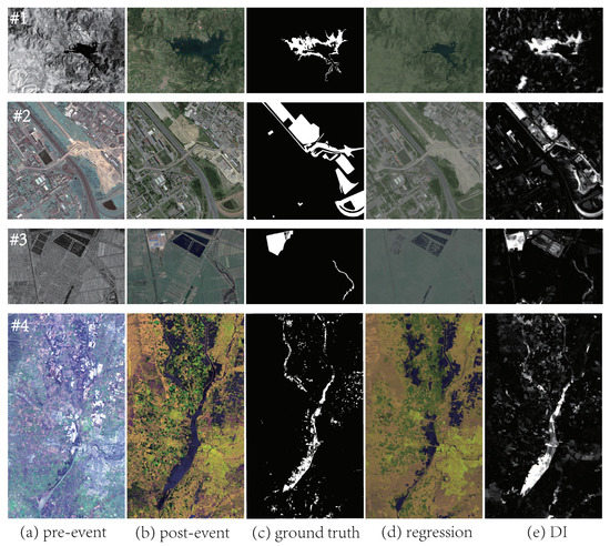
Figure 2. Heterogeneous datasets, regression images and DIs. From top to bottom, they correspond to Datasets #1 to #4, respectively. From left to right: (a) pre-event image $\tilde{\mathbf{X}}$; (b) post-event image $\tilde{\mathbf{Y}}$; (c) the ground truth; (d) the regression images $\tilde{\mathbf{Z}}$; (e) the DI calculated by using (33) with changed feature matrix $\Delta$.

Two types of metrics are utilized to evaluate change detection results. First, the quality of DI is evaluated by the precision-recall (PR) curve and empirical receiver operating characteristics (ROC) curve, which are plotted with the precision rate vs. recall rate and the true positive rate (TPR) vs. false positive rate (FPR), respectively. The precision rate, recall rate (also is the TPR), and FPR are calculated by Precision = TP/(TP + FP), Recall = TP/(TP + FN), and FPR = FP/(TN + FP) respectively, with the true positives, false positives, true negatives, and false negatives abbreviated as TP, FP, TN, and FN, respectively. Second, the quality of binary CM is evaluated by the overall accuracy (OA), the Kappa coefficient ($\kappa$) and F1-score (F1), which are computed as

$$\begin{array}{cc}\hfill & \mathrm{OA}=\frac{\mathrm{TP}+\mathrm{TN}}{\mathrm{TP}+\mathrm{TN}+\mathrm{FP}+\mathrm{FN}}\hfill \\ \hfill & \kappa =\frac{2\times \left(\mathrm{TP}\times \mathrm{TN}-\mathrm{FN}\times \mathrm{FP}\right)}{\left(\mathrm{TP}+\mathrm{FP}\right)\times \left(\mathrm{FP}+\mathrm{TN}\right)+\left(\mathrm{TP}+\mathrm{FN}\right)\times \left(\mathrm{FN}+\mathrm{TN}\right)}\hfill \\ \hfill & \mathrm{F}1=\frac{2\times \mathrm{TP}}{2\times \mathrm{TP}+\mathrm{FP}+\mathrm{FN}}\hfill \end{array}$$

(34)

For all the experiments of AWSG, we choose the global self-expression penalty term as $g\left({\epsilon }^m\right)={∥{\epsilon }^m∥}_F^2$ for Algorithms 1 and 2; we adjust the scale parameter of FNEA to make the number of segmented superpixels around 5000, i.e., $N\approx 5000$, and extract the features of mean, median, and variance values for each band of the superpixel; we fix $\beta =1$, ${\mu }_1={\mu }_2=0.4$ for Algorithms 1 and 2; we set $\lambda =0.1$ and fix $K=3$ (according to the HCD-GSP [42]) for Algorithm 2.

4.2. Regression Images and Difference Images

In the first experiment, we demonstrate the effectiveness of the AWSG-based regression model by displaying the regression image $\tilde{\mathbf{Z}}$ (using the mean feature of $\mathbf{Z}$ as the value of each pixel within the superpixel) and the difference image computed by (33). In Figure 2d, we show the regression images generated by the AWSG on different heterogeneous datasets. We can find that the structures of the regression images $\tilde{\mathbf{Z}}$ are consistent with the pre-event images $\tilde{\mathbf{X}}$ in both the changed and unchanged areas. At the same time, it can also be found that the regression images $\tilde{\mathbf{Z}}$ have the same image style as the post-event images $\tilde{\mathbf{Y}}$. These two aspects demonstrate that the AWSG-based regression model can well translate the pre-event image to the domain of post-event image.

In Figure 2e, we show the DI generated by AWSG on Datasets #1 to #4. There are two observations that can be visualized: first, the DIs are able to distinguish the unchanged and changed areas by giving a larger value to the changed superpixels, which shows the effectiveness of the AWSG-based structure representation of Algorithm 1 and the high-order-based structure regression with the learned AWSG of Algorithm 2; second, the DIs are sparse with the change sparsity-based ${\sum }_{m=1}^M{∥{\Delta }^m∥}_{2,1}$ in the regression model (29), which means that satisfactory segmentation maps can be obtained even by the simple thresholding methods or clustering methods. Figure 3 plots the ROC and PR curves of the difference images, the areas under the ROC curves (AUR) of Datasets #1 to #4 are 0.938, 0.828, 0.954, and 0.878, respectively, and the the areas under the PR curves (AUP) of Datasets #1 to #4 are 0.656, 0.586, 0.735, and 0.456, respectively. From the curves in Figure 3 and the values of AUR and AUP, we can find that the DIs are able to distinguish well between changed and unchanged areas, by simply using the commonly used classification methods, such as thresholding methods (e.g., the Otsu threshold [53]), and clustering methods (e.g., the K-means [54] and fuzzy c-means [55]). For example, if we plot a line with $\mathrm{Precision}=\mathrm{Recall}$ on the PR curves of Figure 3b and calculate the intersection of this diagonal line with the PR curve of each dataset, we can obtain the horizontal coordinates of the points with $\mathrm{Precision}=\mathrm{Recall}$ on the PR curves: 0.689, 0.563, 0.661, 0.519 corresponding to Datasets #1 to #4, respectively. These are also the F1 values ($\mathrm{F}1=\mathrm{Precision}$ when $\mathrm{Precision}=\mathrm{Recall}$) that can be obtained by a simple threshold segmentation on the DIs. From the DIs of Figure 2 and the ROC, PR curves of Figure 3, we can find that the proposed method is able to effectively identify changes from heterogenous image pairs.

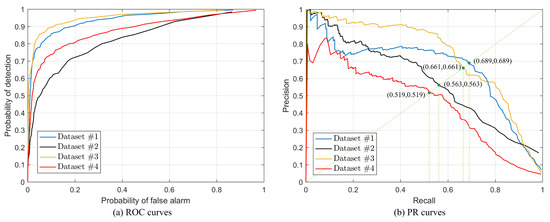
Figure 3. ROC (a) and PR (b) curves of AWSG generated DIs.

4.3. Change Maps

In order to evaluate the effectiveness of the AWSG based HCD algorithm, we select seven SOTA methods (including two deep-learning-based methods) for comparison, where we use the default parameters in the codes that are also consistent with their original papers.

M3CD (M3CD is available at http://www-labs.iro.umontreal.ca/~mignotte (accessed on 9 August 2022)) [16]. An MRF-based method that builds up the observation field from a pixel pairwise modeling and solves the energy minimization problem by using iterative conditional estimation.

FPMS (FPMS is available at http://www-labs.iro.umontreal.ca/~mignotte (accessed on 9 August 2022)) [15]. A fractal projection and Markovian segmentation-based method that translates the image by using a spatial fractal decomposition and a contractive projection.

CICM (CICM is available at http://www-labs.iro.umontreal.ca/~mignotte (accessed on 9 August 2022)) [56]. It is a circular invariant convolution model-based method that aims at transforming images by using a concentric circular invariant convolution representation and a multiscale Markov segmentation model.

SCASC (SCASC is available at https://github.com/yulisun/SCASC (accessed on 9 August 2022)) [10]. It is a sparse-constrained adaptive structure consistency-based method that translates the images by using the structure consistency with a local similarity based graph.

AGSCC (AGSCC is available at https://github.com/yulisun/AGSCC (accessed on 9 August 2022)) [9]. It is an adaptive graph with a structure cycle consistency-based method that translates the images by combining the forward transformation and cycle transformation.

SCCN (SCCN is implemented at https://github.com/llu025 (accessed on 9 August 2022)) [22]. It is a deep-learning-based method that uses a symmetric convolutional coupling network (SCCN) to transform the heterogeneous images into a common feature space.

ACE-Net (ACE-Net is available at https://github.com/llu025 (accessed on 9 August 2022)) [21]. It is a deep image translation method that uses an adversarial cyclic encoder network consisting of two auto-encoders and an affinity-based change prior for network training.

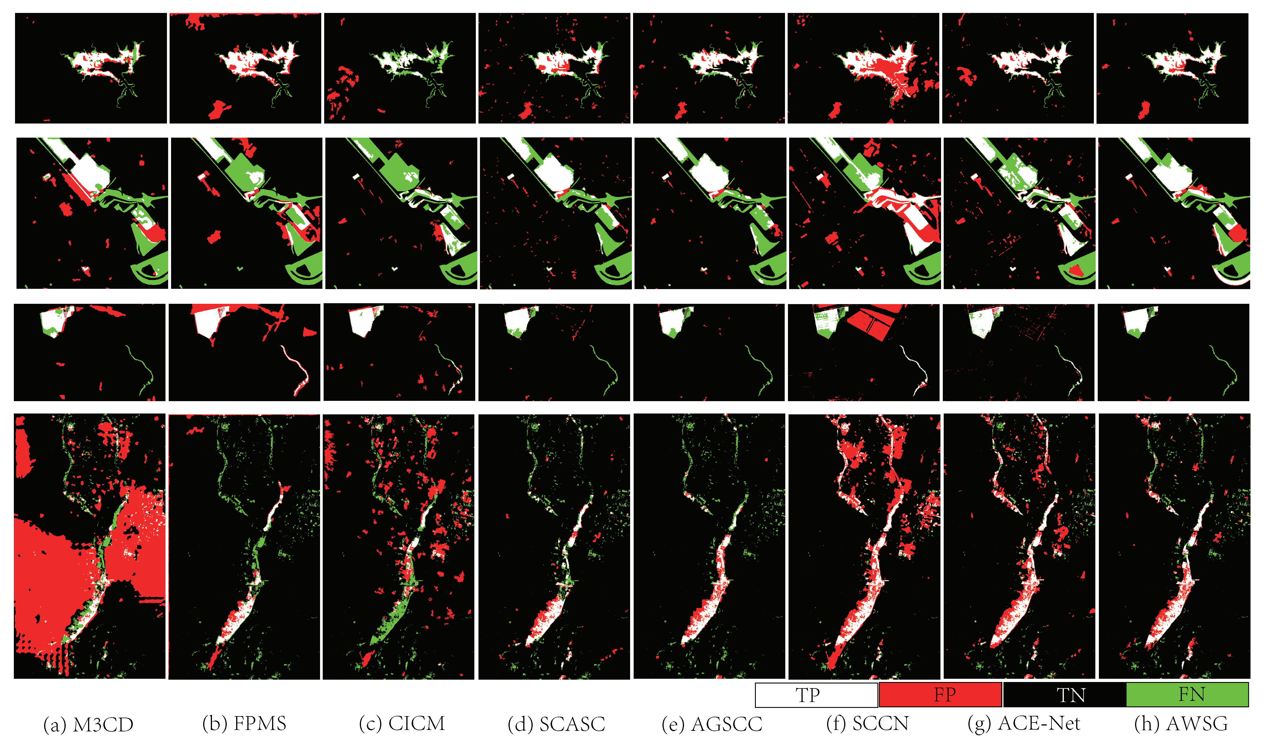
Figure 4 shows the CMs of all the methods on the Datasets #1 to #4, and Table 2 lists the quantitative measures of these CMs. We find that most methods can roughly reflect the change information, whereas some methods do not perform robustly enough on some datasets. To be specific, in Dataset #1, most methods can well identify the changes, but the false negatives in CICM and SCASC are more than for other methods, and the false positives in the SCCN and FPMS are more than others, which leads to a lower F1 and $\kappa$ of CICM, SCCN, FPMS, and SCASC in Table 2. In Dataset #2, the resolution of the multitemporal images is very high (0.52 m) and the proportion of the changed region is also relatively larger than in other datasets, which bring difficulties in accurately detecting changes. From Figure 4 and Table 2, we find that most methods can only detect a small part of the changes, such as FPMS ($\kappa =0.215$) and CICM ($\kappa =0.270$), however, the proposed AWSG can obtain a more accurate CM with better visual effects and highest evaluation metrics ($\kappa =0.524$). In Dataset #3, there are a large number of false alarms in the SCCN, resulting in a poorer detection performance ($\mathrm{F}1=0.386$) than other methods. Additionally, the proposed AWSG is able to obtain good detection results on this dataset, scoring second only to the ACE-Net. In the last Dataset #4, there are more types of objects in the pre- and post-event images than in the other datasets (such as buildings, farmland, rivers, forests, roads, mountains) and these objects are very unevenly proportioned, as shown in Figure 2, which poses difficulties in capturing image structure and completing image regression. Nevertheless, the proposed method is still able to achieve optimal detection results and gain the highest evaluation metrics ($\mathrm{F}1=0.547$), which further demonstrates the structural expressiveness of AWSG and the importance of higher-order structure information in the image regression model. The average OA, $\kappa$ and F1 of the proposed AWSG on these four datasets are about 0.951, 0.628, and 0.656, respectively, which shows that the proposed AWSG is very competitive, even compared with the deep-learning-based methods.

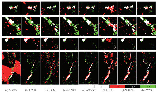
Figure 4. Binary CMs of different methods on heterogeneous datasets. From top to bottom, they correspond to Datasets #1 to #4, respectively. From left to right are binary CMs generated by: (a) M3CD; (b) FPMS; (c) CICM; (d) SCASC; (e) AGSCC; (f) SCCN; (g) ACE-Net; (h) AWSG. In the binary CM, White: true positives (TP); Red: false positives (FP); Black: true negatives (TN); Green: false negatives (FN).

Table 2. Quantitative measures of binary CMs on the heterogeneous datasets. Note that SCCN and ACE-Net are deep-learning-based methods.

Methods	Dataset #1			Dataset #2			Dataset #3			Dataset #4			Average
	OA	$\mathit{\kappa }$	F1	OA	$\mathit{\kappa }$	F1	OA	$\mathit{\kappa }$	F1	OA	$\mathit{\kappa }$	F1	OA	$\mathit{\kappa }$	F1
M3CD	0.963	0.669	0.689	0.863	0.405	0.481	0.962	0.602	0.622	0.575	0.021	0.077	0.841	0.424	0.467
FPMS	0.925	0.552	0.588	0.838	0.215	0.296	0.938	0.569	0.597	0.947	0.329	0.356	0.912	0.416	0.459
CICM	0.943	0.451	0.481	0.867	0.270	0.321	0.974	0.745	0.759	0.899	0.081	0.131	0.921	0.387	0.423
SCASC	0.947	0.593	0.621	0.892	0.464	0.516	0.979	0.741	0.751	0.961	0.479	0.500	0.945	0.569	0.597
AGSCC	0.959	0.658	0.680	0.897	0.490	0.540	0.983	0.773	0.782	0.960	0.486	0.506	0.950	0.602	0.627
SCCN	0.900	0.478	0.524	0.848	0.417	0.507	0.908	0.344	0.386	0.906	0.392	0.431	0.891	0.408	0.462
ACE-Net	0.964	0.718	0.737	0.886	0.480	0.541	0.981	0.788	0.798	0.940	0.468	0.497	0.943	0.614	0.643
AWSG	0.963	0.690	0.711	0.896	0.524	0.581	0.984	0.775	0.783	0.962	0.524	0.547	0.951	0.628	0.656

4.4. Discussion

4.4.1. Ablation Study

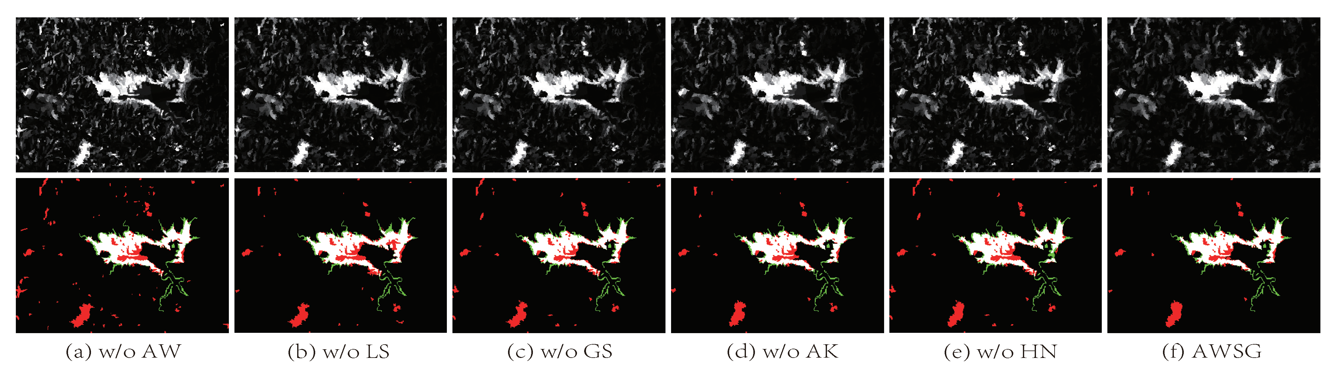
The proposed AWSG mainly contains two processes: the structure representation by learning an auto-weighted structured graph and the structure regression by using high-order neighbor information of the graph. To further investigate the contributions of the proposed method in the heterogeneous CD, that is, the roles of the auto-weighted strategy, the structured graph combining local and global information, the adaptive k-selection strategy, and the high-order structure regression, an ablation experiment is carried out, i.e., eliminating the corresponding parts on the basis of the complete AWSG for comparison. The detection performances (F1 measure of CM) of the AWSG without (w/o) auto-weighted strategy (AW), local structure information (LS), global structure information (GS), adaptive k-selection (AK), high-order neighbor information (HN) are reported in Table 3. In addition, we also show the DI and CM generated by AWSG without these parts on Dataset #1 in Figure 5.

Table 3. Ablation study of AWSG measured by the F1 score of CM.

Methods	Heterogeneous Datasets				Average
	#1	#2	#3	#4
AWSG w/o AW	0.665	0.549	0.751	0.513	0.620
AWSG w/o LS	0.682	0.564	0.761	0.525	0.633
AWSG w/o GS	0.695	0.558	0.752	0.540	0.636
AWSG w/o AK	0.703	0.570	0.772	0.521	0.642
AWSG w/o HN	0.677	0.565	0.760	0.539	0.635
AWSG	0.711	0.581	0.783	0.547	0.656

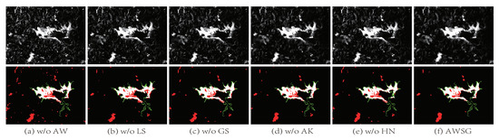
Figure 5. Ablation study of AWSG. From top to bottom, they correspond to the DI and CM generated by different methods on the Dataset #1. From left to right are the results generated by: (a) AWSG without auto-weighted strategy; (b) AWSG without local structure information; (c) AWSG without global structure information; (d) AWSG without adaptive k-selection; (e) AWSG without high-order neighbor information; (f) the original AWSG.

According to Table 3, the detection performance degrades without (w/o) AW, LS, GS, AK, and HN on all the evaluated datasets. Specifically, compared to the other parts, the effect of adaptive k-selection structure is slightly weaker, which has a more pronounced effect on datasets with uneven feature distribution, e.g., the F1 score is improved by 2.6% in Dataset #4. When applied with the auto-weighted strategy, the constructed graph can adaptively assign different weights for different features by using a self-conducted weight learning, which makes the graph more robust. Therefore, the score of F1 increases by about 4.6% on Dataset #1 and 3.2% on Dataset #2 compared to that without AW. By using the structured graph that combines the local similarity structure and global self-expression property, the average score of the F1 is about 2.0% higher than that of using only local structural information and 2.3% higher than that of using only global structural information as reported by Table 3. It can also be seen in Figure 5 that the CM of AWSG combining global and local structure information has fewer false alarms and missed detections than the AWSG w/o LS or GS, which demonstrates the effectiveness of structured graph that can improve the ability of characterizing structures. By exploiting the high-order neighbor information ($\mathcal{H}\left(\mathbf{L}\right)$ and $\mathcal{H}\left(\mathbf{S}\right)$) in the structure regression model (29), the final detection results is more accurate, as shown in Figure 5e,f, and the average F1 can be improved by about 2.1% compared to that which only uses the first-order neighborhood information, as reported in Table 3.

4.4.2. Parameter Analysis

The main parameters of AWSG are the superpixel number N, maximum iterations $N_{iter}$, the balancing parameter $\beta$, and the sparse penalty parameter $\lambda$.

Generally, the number N of superpixels should be determined based on the resolution of the dataset and should also take into account the CD task’s requirements on computational efficiency. A large N increases the computational burden while improving the detection granularity.

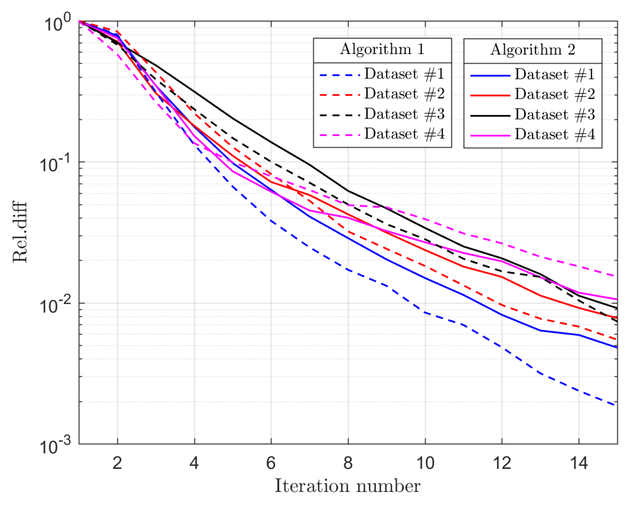
To investigate the convergence performance of the proposed AWSG with parameter $N_{iter}$, we plot the convergence curves of Algorithms 1 and 2, which are measured by the relative difference (Rel.diff) ${\xi }^k$ versus iteration number k, as shown in Figure 6, where ${\xi }^{[k+1]}=\sum _{m=1}^M\frac{{∥{\mathbf{S}}^{[k+1]}-{\mathbf{S}}^{\left[k\right]}∥}_F}{{∥{\mathbf{S}}^{[k+1]}∥}_F}$ for the Algorithm 1 and ${\xi }^{[k+1]}=\sum _{m=1}^M\frac{{∥{\Delta }^{m[k+1]}-{\Delta }^{m\left[k\right]}∥}_F}{{∥{\Delta }^{m[k+1]}∥}_F}$ for the Algorithm 2. It is clear that the ADMM in the solving of Algorithms 1 and 2 converges quickly, and the exit criterion of $N_{iter}=15$ or ${\xi }^0=0.01$ is enough for the algorithms when taking into account the computational time.

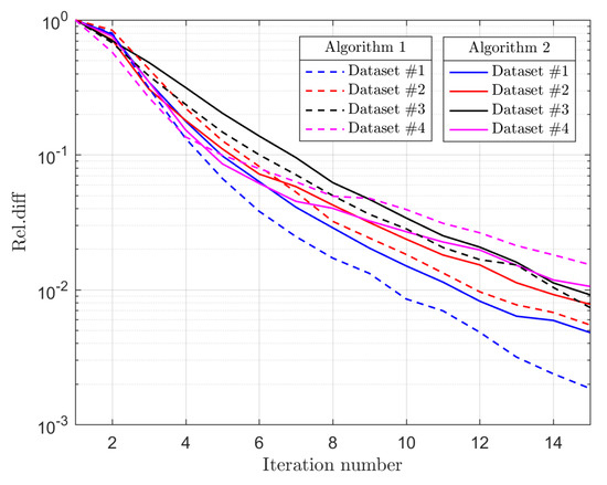
Figure 6. Convergence performance of AWSG.

The parameter $\beta$ balances the weight of local structure penalty term and global self-expression penalty term in the graph learning model (5) and structure regression model (29). Given the penalty function of $g\left({\epsilon }^m\right)={∥{\epsilon }^m∥}_F^2$, we have ${\sum }_{i=1}^N{\sum }_{j=1}^N{∥{\mathbf{X}}_i^m-{\mathbf{X}}_j^m∥}_2^2{S}_{i,j}\ge {∥{\mathbf{X}}^m-{\mathbf{X}}^m\mathbf{S}∥}_F^2$ by using the condition of ${\sum }_{i=1}^N{S}_{i,j}=1$. Therefore, it is recommended that $\beta \ge 1$.

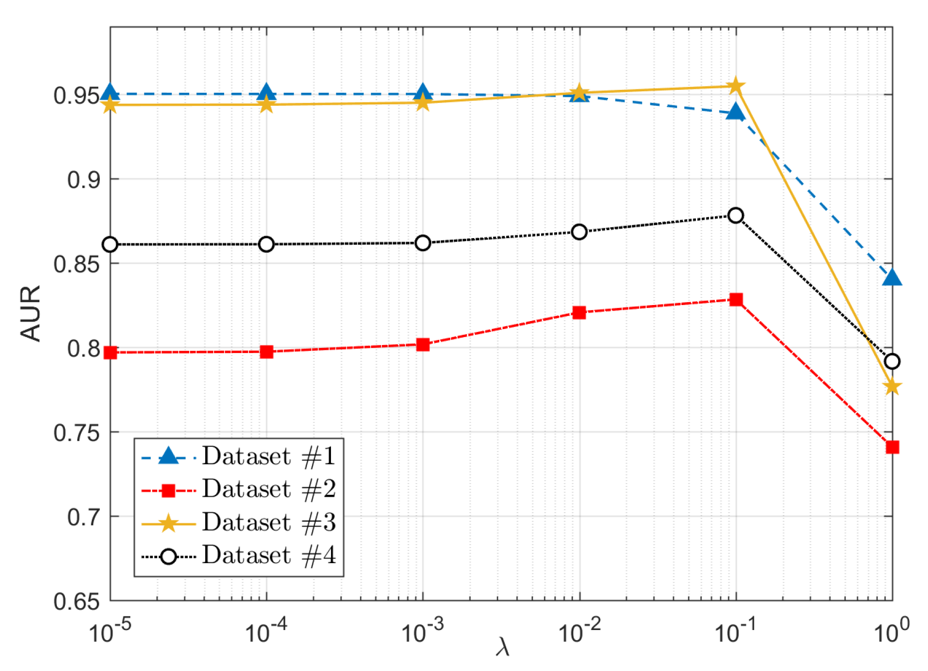
For the sparse penalty parameter $\lambda$, it is used to control the sparsity level of DI, which should be determined based on the percentage of real change in the ground truth. However, we experimentally find that the proposed algorithm is not sensitive to this parameter, as shown in Figure 7, where we show the AUR at different values of $\lambda$ (from ${10}^{-5}$ to 1 with the ratio of 10). It can be found that the AWSG performs well in a broad range of $\lambda$.

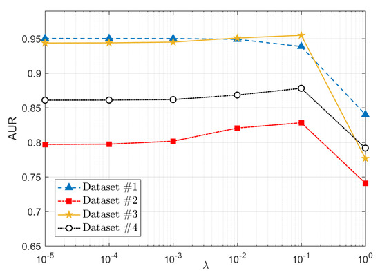
Figure 7. Influence of parameter $\lambda$ on the proposed AWSG.

4.4.3. Complexity Analysis

The main complexity of the proposed method is concentrated in the AWSG learning (Algorithm 1) and the structure regression with AWSG (Algorithm 2).

Algorithm 1: Step 1, update ${\epsilon }^m$, requires $\mathcal{O}\left(C_x{N}^2\right)$ for calculating ${\mathbf{Q}}^m$ and $\mathcal{O}\left(C_{x}N\right)$ for the proximal operator of (14); Step 2, update $\mathbf{P}$, requires $\mathcal{O}\left(N^3\right)$ for the matrix inversion of ${\left({\mathbf{I}}_N+\frac{{\mu }_1}{{\mu }_2}{\sum }_{m=1}^M{\left({\mathbf{X}}^m\right)}^T{\mathbf{X}}^m\right)}^{-1}$ and $\mathcal{O}\left(C_x{N}^2\right)$ for the matrix multiplication; Step 3, update $\mathbf{S}$, requires $\mathcal{O}\left(C_x{N}^2\right)$ for calculating $\mathbf{E}$, $\mathcal{O}\left(N^{2}logN\right)$ for sorting all columns of $\mathbf{E}$, and $\mathcal{O}\left(N^2\right)$ for the closed-form solution of (22); Step 4, update $w_m$, requires $\mathcal{O}\left(N^2\right)$ by using (8) or (24); Step 5, update the Lagrangian multipliers of ${\mathbf{R}}_1$ and ${\mathbf{R}}_2^m$, requires $\mathcal{O}\left(C_x{N}^2\right)$ for matrix multiplication.

Algorithm 2: Step 1, update ${\epsilon }^m$, requires $\mathcal{O}\left(C_y{N}^2\right)$ for the matrix multiplication and $\mathcal{O}\left(C_{y}N\right)$ for the proximal operator of (31a); Step 2, update ${\Delta }^m$, requires $\mathcal{O}\left(C_{y}N\right)$ by using (31b); Step 3, update ${\mathbf{Z}}^m$, requires for $\mathcal{O}\left(C_y{N}^2\right)$ calculating ${\Theta }^m$, $\mathcal{O}\left(N^3\right)$ for the matrix inversion of ${\Psi }^{-1}$, and $\mathcal{O}\left(C_y{N}^2\right)$ for the matrix multiplication; Step 4, update $w_m$, requires $\mathcal{O}\left(N^2\right)$ by using (31d); Step 5, update the Lagrangian multipliers of ${\mathbf{R}}_1^m$ and ${\mathbf{R}}_2^m$, requires $\mathcal{O}\left(C_y{N}^2\right)$ for the matrix multiplication.

Although the complexity of AWSG is very high in the above theoretical analysis, which requires $\mathcal{O}\left(N^3\right)$ for the matrix inversion of each iteration in Algorithms 1 and 2, it can be accelerated by using some iterative solvers for updating $\mathbf{P}$ with (19) in Algorithm 1 and ${\mathbf{Z}}^m$ with (31c) in Algorithm 2. The linear systems of updating $\mathbf{P}$ and ${\mathbf{Z}}^m$ can be solved efficiently by using the conjugate gradient (CG) method. In addition, some pre-conditioners can also be used to accelerate CG method [57]. In our experiments, we use the CG with incomplete Cholesky pre-conditioner for updating $\mathbf{P}$ and ${\mathbf{Z}}^m$. The computational time of each process of AWSG with different N on Datasets #2 and #3 is listed in Table 4, where the AWSG is performed in MATLAB 2016a running with Intel Core i9-10980HK CPU.

Table 4. Computational time (s) of AWSG, where $t_{A1}$, $t_{A2}$, and $t_{total}$ denote the computational time of Algorithms 1 and 2 and the whole AWSG, respectively.

Datasets	N	${\mathit{t}}_{\mathit{A}1}$	${\mathit{t}}_{\mathit{A}2}$	${\mathit{t}}_{\mathbf{total}}$
Dataset #2 $2000\times 2000\times 3\left(3\right)$	2500	3.8	2.0	9.1
	5000	12.1	5.9	29.3
	10,000	69.8	28.7	127.5
Dataset #3 $593\times 921\times 1\left(3\right)$	2500	3.5	1.8	8.4
	5000	10.4	5.1	24.2
	10,000	65.9	26.6	120.4

5. Conclusions

In this paper, we proposed an unsupervised image regression method for heterogeneous change detection. Specifically, the proposed method first segments the multitemporal images into superpixels, and learns an adaptive KNN graph for the pre-event image to capture the structure information, which uses a self-conducted weighting strategy and combines the local and global structure information to make the graph more capable of structural characterization. Then, based on the structure consistency between heterogeneous images, the proposed method transforms the pre-event image to the domain of post-event image by using the learned graph. By exploiting the high-order neighbor information hidden in the graph, it can obtain a better translated image and change image and thus improve the accuracy of change detection. The experimental results confirm the effectiveness of the proposed method by comparing with other related methods. In future work, we will focus on the distributional properties of the image, especially ways to improve the structure representation of the graph in the case of uneven object distribution.

References

- Singh, A. Review Article Digital change detection techniques using remotely-sensed data. Int. J. Remote Sens. 1989, 10, 989–1003. [Google Scholar] [CrossRef]
- Liu, S.; Marinelli, D.; Bruzzone, L.; Bovolo, F. A Review of Change Detection in Multitemporal Hyperspectral Images: Current Techniques, Applications, and Challenges. IEEE Geosci. Remote Sens. Mag. 2019, 7, 140–158. [Google Scholar] [CrossRef]
- Lv, Z.; Liu, T.; Benediktsson, J.A.; Falco, N. Land Cover Change Detection Techniques: Very-High-Resolution Optical Images: A Review. IEEE Geosci. Remote Sens. Mag. 2021, 10, 2–21. [Google Scholar] [CrossRef]
- Wen, D.; Huang, X.; Bovolo, F.; Li, J.; Ke, X.; Zhang, A.; Benediktsson, J.A. Change Detection From Very-High-Spatial-Resolution Optical Remote Sensing Images: Methods, applications, and future directions. IEEE Geosci. Remote Sens. Mag. 2021, 9, 68–101. [Google Scholar] [CrossRef]
- Moser, G.; Serpico, S. Generalized minimum-error thresholding for unsupervised change detection from SAR amplitude imagery. IEEE Trans. Geosci. Remote Sens. 2006, 44, 2972–2982. [Google Scholar] [CrossRef]
- Lv, Z.; Liu, T.; Shi, C.; Benediktsson, J.A. Local Histogram-Based Analysis for Detecting Land Cover Change Using VHR Remote Sensing Images. IEEE Geosci. Remote Sens. Lett. 2021, 18, 1284–1287. [Google Scholar] [CrossRef]
- Lv, Z.; Wang, F.; Cui, G.; Benediktsson, J.A.; Lei, T.; Sun, W. Spatial-Spectral Attention Network Guided with Change Magnitude Image for Land Cover Change Detection Using Remote Sensing Images. IEEE Trans. Geosci. Remote Sens. 2022, 60, 1. [Google Scholar] [CrossRef]
- Wang, Q.; Yuan, Z.; Du, Q.; Li, X. GETNET: A General End-to-End 2-D CNN Framework for Hyperspectral Image Change Detection. IEEE Trans. Geosci. Remote Sens. 2019, 57, 3–13. [Google Scholar] [CrossRef]
- Sun, Y.; Lei, L.; Guan, D.; Wu, J.; Kuang, G.; Liu, L. Image Regression With Structure Cycle Consistency for Heterogeneous Change Detection. IEEE Trans. Neural Netw. Learn. Syst. 2022, 1–15. [Google Scholar] [CrossRef]
- Sun, Y.; Lei, L.; Guan, D.; Li, M.; Kuang, G. Sparse-Constrained Adaptive Structure Consistency-Based Unsupervised Image Regression for Heterogeneous Remote Sensing Change Detection. IEEE Trans. Geosci. Remote Sens. 2021, 60, 1–14. [Google Scholar] [CrossRef]
- Deng, W.; Liao, Q.; Zhao, L.; Guo, D.; Kuang, G.; Hu, D.; Liu, L. Joint Clustering and Discriminative Feature Alignment for Unsupervised Domain Adaptation. IEEE Trans. Image Process. 2021, 30, 7842–7855. [Google Scholar] [CrossRef] [PubMed]
- Deng, W.; Zhao, L.; Kuang, G.; Hu, D.; Pietikäinen, M.; Liu, L. Deep Ladder-Suppression Network for Unsupervised Domain Adaptation. IEEE Trans. Cybern. 2021, 1–15. [Google Scholar] [CrossRef] [PubMed]
- Deng, W.; Cui, Y.; Liu, Z.; Kuang, G.; Hu, D.; Pietikäinen, M.; Liu, L. Informative Class-Conditioned Feature Alignment for Unsupervised Domain Adaptation. In Proceedings of the 29th ACM International Conference on Multimedia, Nice, France, 21–25 October 2021; pp. 1303–1312. [Google Scholar]
- Luppino, L.T.; Bianchi, F.M.; Moser, G.; Anfinsen, S.N. Unsupervised Image Regression for Heterogeneous Change Detection. IEEE Trans. Geosci. Remote Sens. 2019, 57, 9960–9975. [Google Scholar] [CrossRef]
- Mignotte, M. A Fractal Projection and Markovian Segmentation-Based Approach for Multimodal Change Detection. IEEE Trans. Geosci. Remote Sens. 2020, 58, 8046–8058. [Google Scholar] [CrossRef]
- Touati, R.; Mignotte, M.; Dahmane, M. Multimodal Change Detection in Remote Sensing Images Using an Unsupervised Pixel Pairwise-Based Markov Random Field Model. IEEE Trans. Image Process. 2020, 29, 757–767. [Google Scholar] [CrossRef]
- Liu, Z.; Li, G.; Mercier, G.; He, Y.; Pan, Q. Change Detection in Heterogenous Remote Sensing Images via Homogeneous Pixel Transformation. IEEE Trans. Image Process. 2018, 27, 1822–1834. [Google Scholar] [CrossRef]
- Li, X.; Du, Z.; Huang, Y.; Tan, Z. A deep translation (GAN) based change detection network for optical and SAR remote sensing images. ISPRS J. Photogramm. Remote Sens. 2021, 179, 14–34. [Google Scholar] [CrossRef]
- Lv, Z.; Huang, H.; Gao, L.; Benediktsson, J.A.; Zhao, M.; Shi, C. Simple Multiscale UNet for Change Detection With Heterogeneous Remote Sensing Images. IEEE Geosci. Remote Sens. Lett. 2022, 19, 1–5. [Google Scholar] [CrossRef]
- Lv, Z.; Li, G.; Jin, Z.; Benediktsson, J.A.; Foody, G.M. Iterative Training Sample Expansion to Increase and Balance the Accuracy of Land Classification From VHR Imagery. IEEE Trans. Geosci. Remote Sens. 2021, 59, 139–150. [Google Scholar] [CrossRef]
- Luppino, L.T.; Kampffmeyer, M.; Bianchi, F.M.; Moser, G.; Serpico, S.B.; Jenssen, R.; Anfinsen, S.N. Deep Image Translation With an Affinity-Based Change Prior for Unsupervised Multimodal Change Detection. IEEE Trans. Geosci. Remote Sens. 2022, 60, 1–22. [Google Scholar] [CrossRef]
- Liu, J.; Gong, M.; Qin, K.; Zhang, P. A Deep Convolutional Coupling Network for Change Detection Based on Heterogeneous Optical and Radar Images. IEEE Trans. Neural Netw. Learn. Syst. 2018, 29, 545–559. [Google Scholar] [CrossRef] [PubMed]
- Sun, Y.; Lei, L.; Guan, D.; Kuang, G. Iterative Robust Graph for Unsupervised Change Detection of Heterogeneous Remote Sensing Images. IEEE Trans. Image Process. 2021, 30, 6277–6291. [Google Scholar] [CrossRef] [PubMed]
- Touati, R.; Mignotte, M. An Energy-Based Model Encoding Nonlocal Pairwise Pixel Interactions for Multisensor Change Detection. IEEE Trans. Geosci. Remote Sens. 2018, 56, 1046–1058. [Google Scholar] [CrossRef]
- Gong, M.; Zhang, P.; Su, L.; Liu, J. Coupled Dictionary Learning for Change Detection From Multisource Data. IEEE Trans. Geosci. Remote Sens. 2016, 54, 7077–7091. [Google Scholar] [CrossRef]
- Mercier, G.; Moser, G.; Serpico, S.B. Conditional Copulas for Change Detection in Heterogeneous Remote Sensing Images. IEEE Trans. Geosci. Remote Sens. 2008, 46, 1428–1441. [Google Scholar] [CrossRef]
- Sun, Y.; Lei, L.; Li, X.; Tan, X.; Kuang, G. Patch Similarity Graph Matrix-Based Unsupervised Remote Sensing Change Detection With Homogeneous and Heterogeneous Sensors. IEEE Trans. Geosci. Remote Sens. 2021, 59, 4841–4861. [Google Scholar] [CrossRef]
- Sun, Y.; Lei, L.; Li, X.; Tan, X.; Kuang, G. Structure Consistency-Based Graph for Unsupervised Change Detection With Homogeneous and Heterogeneous Remote Sensing Images. IEEE Trans. Geosci. Remote Sens. 2021, 60, 1–21. [Google Scholar] [CrossRef]
- Prendes, J.; Chabert, M.; Pascal, F.; Giros, A.; Tourneret, J.Y. A New Multivariate Statistical Model for Change Detection in Images Acquired by Homogeneous and Heterogeneous Sensors. IEEE Trans. Image Process. 2015, 24, 799–812. [Google Scholar] [CrossRef]
- Volpi, M.; Camps-Valls, G.; Tuia, D. Spectral alignment of multi-temporal cross-sensor images with automated kernel canonical correlation analysis. ISPRS J. Photogramm. Remote Sens. 2015, 107, 50–63. [Google Scholar] [CrossRef]
- Sun, Y.; Lei, L.; Tan, X.; Guan, D.; Wu, J.; Kuang, G. Structured graph based image regression for unsupervised multimodal change detection. ISPRS J. Photogramm. Remote Sens. 2022, 185, 16–31. [Google Scholar] [CrossRef]
- Jiang, X.; Li, G.; Liu, Y.; Zhang, X.P.; He, Y. Change Detection in Heterogeneous Optical and SAR Remote Sensing Images Via Deep Homogeneous Feature Fusion. IEEE J. Sel. Top. Appl. Earth Obs. Remote Sens. 2020, 13, 1551–1566. [Google Scholar] [CrossRef]
- Liu, Z.; Zhang, Z.; Pan, Q.; Ning, L. Unsupervised Change Detection From Heterogeneous Data Based on Image Translation. IEEE Trans. Geosci. Remote Sens. 2022, 60, 1–13. [Google Scholar] [CrossRef]
- Wu, Y.; Li, J.; Yuan, Y.; Qin, A.K.; Miao, Q.G.; Gong, M.G. Commonality Autoencoder: Learning Common Features for Change Detection From Heterogeneous Images. IEEE Trans. Neural Netw. Learn. Syst. 2021, 33, 1–14. [Google Scholar] [CrossRef]
- Saha, S.; Ebel, P.; Zhu, X.X. Self-Supervised Multisensor Change Detection. IEEE Trans. Geosci. Remote Sens. 2022, 60, 1–10. [Google Scholar] [CrossRef]
- Chen, Y.; Bruzzone, L. Self-Supervised Change Detection in Multiview Remote Sensing Images. IEEE Trans. Geosci. Remote Sens. 2022, 60, 1–12. [Google Scholar] [CrossRef]
- Wu, J.; Li, B.; Qin, Y.; Ni, W.; Zhang, H.; Fu, R.; Sun, Y. A multiscale graph convolutional network for change detection in homogeneous and heterogeneous remote sensing images. Int. J. Appl. Earth Obs. Geoinf. 2021, 105, 102615. [Google Scholar] [CrossRef]
- Jimenez-Sierra, D.A.; Benítez-Restrepo, H.D.; Vargas-Cardona, H.D.; Chanussot, J. Graph-Based Data Fusion Applied to: Change Detection and Biomass Estimation in Rice Crops. Remote Sens. 2020, 12, 2683. [Google Scholar] [CrossRef]
- Jimenez-Sierra, D.A.; Quintero-Olaya, D.A.; Alvear-Muñoz, J.C.; Benítez-Restrepo, H.D.; Florez-Ospina, J.F.; Chanussot, J. Graph Learning Based on Signal Smoothness Representation for Homogeneous and Heterogeneous Change Detection. IEEE Trans. Geosci. Remote Sens. 2022, 60, 1–16. [Google Scholar] [CrossRef]
- Sun, Y.; Lei, L.; Li, X.; Sun, H.; Kuang, G. Nonlocal patch similarity based heterogeneous remote sensing change detection. Pattern Recognit. 2021, 109, 107598. [Google Scholar] [CrossRef]
- Sun, Y.; Lei, L.; Guan, D.; Kuang, G.; Liu, L. Graph Signal Processing for Heterogeneous Change Detection–Part I: Vertex Domain Filtering. arXiv 2022, arXiv:2208.01881. [Google Scholar] [CrossRef]
- Sun, Y.; Lei, L.; Guan, D.; Kuang, G.; Liu, L. Graph Signal Processing for Heterogeneous Change Detection–Part II: Spectral Domain Analysis. arXiv 2022, arXiv:2208.01905. [Google Scholar] [CrossRef]
- Baatz, M. Multi resolution segmentation: An optimum approach for high quality multi scale image segmentation. In Proceedings of the Beutrage zum AGIT-Symposium; Springer: Salzburg, Germany, 2000; pp. 12–23. [Google Scholar]
- Zhou, D.; Bousquet, O.; Lal, T.N.; Weston, J.; Schölkopf, B. Learning with local and global consistency. Adv. Neural Inf. Process. Syst. 2004, 16, 321–328. [Google Scholar]
- Wang, F.; Zhang, C.; Li, T. Clustering with local and global regularization. IEEE Trans. Knowl. Data Eng. 2009, 21, 1665–1678. [Google Scholar] [CrossRef]
- Kang, Z.; Peng, C.; Cheng, Q.; Liu, X.; Peng, X.; Xu, Z.; Tian, L. Structured graph learning for clustering and semi-supervised classification. Pattern Recognit. 2021, 110, 107627. [Google Scholar] [CrossRef]
- Zhu, X.; Li, X.; Zhang, S.; Ju, C.; Wu, X. Robust joint graph sparse coding for unsupervised spectral feature selection. IEEE Trans. Neural Netw. Learn. Syst. 2016, 28, 1263–1275. [Google Scholar] [CrossRef]
- Nie, F.; Li, J.; Li, X. Parameter-free auto-weighted multiple graph learning: A framework for multiview clustering and semi-supervised classification. In Proceedings of the Twenty-Fifth International Joint Conference on Artificial Intelligence, New York, NY, USA, 9–15 July 2016; pp. 1881–1887. [Google Scholar]
- Yang, J.; Yin, W.; Zhang, Y.; Wang, Y. A fast algorithm for edge-preserving variational multichannel image restoration. SIAM J. Imaging Sci. 2009, 2, 569–592. [Google Scholar] [CrossRef]
- Zhang, X.; Ying, W.; Yang, P.; Sun, M. Parameter estimation of underwater impulsive noise with the Class B model. IET Radar Sonar Navig. 2020, 14, 1055–1060. [Google Scholar] [CrossRef]
- Mahmood, A.; Chitre, M. Modeling colored impulsive noise by Markov chains and alpha-stable processes. In Proceedings of the OCEANS 2015, Genova, Italy, 18–21 May 2015; pp. 1–7. [Google Scholar]
- Nie, F.; Wang, X.; Huang, H. Clustering and projected clustering with adaptive neighbors. In Proceedings of the 20th ACM SIGKDD International Conference on Knowledge discovery and Data Mining, New York, NY, USA, 24–27 August 2014; pp. 977–986. [Google Scholar]
- Otsu, N. A threshold selection method from gray-level histograms. IEEE Trans. Syst. Man Cybern. 1979, 9, 62–66. [Google Scholar] [CrossRef]
- Hartigan, J.A.; Wong, M.A. Algorithm AS 136: A k-means clustering algorithm. J. R. Stat. Soc. Ser. C (Appl. Stat.) 1979, 28, 100–108. [Google Scholar] [CrossRef]
- Bezdek, J.C.; Ehrlich, R.; Full, W. FCM: The fuzzy c-means clustering algorithm. Comput. Geosci. 1984, 10, 191–203. [Google Scholar] [CrossRef]
- Touati, R. Détection de Changement en Imagerie Satellitaire Multimodale. Ph.D. Thesis, Université de Montréal, Montréal, QC, Canada, 2019. [Google Scholar]
- Nar, F.; Özgür, A.; Saran, A.N. Sparsity-Driven Change Detection in Multitemporal SAR Images. IEEE Geosci. Remote Sens. Lett. 2016, 13, 1032–1036. [Google Scholar] [CrossRef]
Publisher’s Note: MDPI stays neutral with regard to jurisdictional claims in published maps and institutional affiliations. |
© 2022 by the authors. Licensee MDPI, Basel, Switzerland. This article is an open access article distributed under the terms and conditions of the Creative Commons Attribution (CC BY) license (https://creativecommons.org/licenses/by/4.0/).