Prediction of Sea Surface Temperature by Combining Interdimensional and Self-Attention with Neural Networks

Abstract

Sea surface temperature (SST) is one of the most important and widely used physical parameters for oceanography and meteorology. To obtain SST, in addition to direct measurement, remote sensing, and numerical models, a variety of data-driven models have been developed with a wealth of SST data being accumulated. As oceans are comprehensive and complex dynamic systems, the distribution and variation of SST are affected by various factors. To overcome this challenge and improve the prediction accuracy, a multi-variable long short-term memory (LSTM) model is proposed which takes wind speed and air pressure at sea level together with SST as inputs. Furthermore, two attention mechanisms are introduced to optimize the model. An interdimensional attention strategy, which is similar to the positional encoding matrix, is utilized to focus on important historical moments of multi-dimensional input; a self-attention strategy is adopted to smooth the data during the training process. Forty-three-year monthly mean SST and meteorological data from the fifth-generation ECMWF (European Centre for Medium-Range Weather Forecasts) reanalysis (ERA5) are collected to train and test the model for the sea areas around China. The performance of the model is evaluated in terms of different statistical parameters, namely the coefficient of determination, root mean squared error, mean absolute error and mean average percentage error, with a range of 0.9138–0.991, 0.3928–0.8789, 0.3213–0.6803, and 0.1067–0.2336, respectively. The prediction results indicate that it is superior to the LSTM-only model and models taking SST only as input, and confirm that our model is promising for oceanography and meteorology investigation.

1. Introduction

Sea surface temperature (SST) is the one of the most important and widely used parameters in the analysis of global climate change. It is also used as boundary conditions or assimilation information in the analysis of atmospheric circulation anomalies, atmospheric models, and sea–air coupled models [1]. In addition, SST constitutes important basic data for aquaculture industry environmental assurance [2].

Although observations of SST have a history of more than 200 years, it was not until 1853 when the Brussels International Conference on Nautical Meteorology decided to start the collection of global SST data and standardize the organization and analysis of SST data. In recent decades, SST observation has transitioned through bucket observation measurements, Engine Room Intake (ERI) observations, ship-sensing observations, and satellite remote-sensing observations [3]. The uneven spatial and temporal distribution of observations need to be solved to obtain long-term, accurate global SST information. For this purpose, the reanalysis takes advantage of data assimilation techniques to integrate SST data from various sources and types of observations with numerical forecast products [4]. A number of reanalysis products that provide accurate forecasts across broad spatial and temporal scales have been released. In recent years, there has been a large volume of published studies comparing the products from different aspects. In 2013, Baololqimuge summarized several commonly used SST observation methods and introduced four sets of SST data including the Hadley Centre Sea Ice and Sea Surface Temperature data set (HadISST), the International Comprehensive Ocean-Atmosphere Data Set (ICOADS), Extended Reconstructed Sea Surface Temperature (ERSST) and Optimum Interpolation Sea Surface Temperature Analysis (OISSTA) in detail [3]. In the same year, Jiang conducted a comparative statistical analysis of six different SST products [5]. In 2020, Wang compared the applicability of three sets of reanalysis data around China [6].

The traditional methods for predicting ocean elements are divided into three main categories: numerical models, artificial experience and statistical prediction [4]. Numerical models are obtained under parametric conditions for physical processes in the ocean and are more suited to large sea areas and long-term SST prediction [7]. Furthermore, the computational requirements for ocean simulations are immense and require high-performance computing (HPC) facilities [8]. Artificial empirical and statistical prediction methods are more affected by parameter settings and the degree of human cognition.

Over the years, with the development, launch, and application of a series of satellites for oceanology and meteorology, satellite data have been increasing in magnitude. Additionally, the improvements in ocean models together with increased computational capabilities led to a number of reanalysis data [8]. The accumulation of a large amount of data on marine environmental elements has laid the foundation for data-driven methods [9]. These models abandon the subjectivity of traditional machine learning that requires experts to design and create feature extractors through experiments; they automatically and objectively extract useful information from data. Thus, they bring new opportunities for intelligent analysis and mining of marine data.

SST prediction can essentially be regarded as a time-series regression problem. The traditional models for time-series prediction, such as autoregressive (AR), moving average (MA), the autoregressive integrated moving average model (ARIMA) and the regression model by machine learning, including support vector regression (SVR) [10], and multi-layer perceptron (MLP) have been widely used in SST prediction [11]. An atmospheric reflection Grey model was proposed to predict long-term SST [12]. More recent attention has focused on the deep learning models, which originated from the artificial neural network (ANN). In 2006, Hinton proposed the concept of deep learning, which promoted the implementation of a number of deep learning projects [13]. A recurrent neural network (RNN) is a deep model developed for modeling sequential data [14]. The RNN introduces hidden states to extract features from sequential data and convert them to outputs. Hochreiter proposed the long short-term memory (LSTM) model, which introduces the forgetting gate and the memory gate [15]. In 2017, Zhang first adopted the LSTM model to predict SST. In the same year, based on the convolutional LSTM (ConvLSTM) model [16], Xu proposed a sequence-to-sequence (Seq2Seq)-based regional sea level temperature anomaly prediction model [17]. In 2018, Yang introduced spatial information with the LSTM model to build a model for SST prediction, and applied it effectively in the SST data set of coastal China [18]. In 2019, Zhu applied the LSTM-RNN to SST prediction and constructed a model for SST time-series variation in the western Pacific sea area [19]. LSTM was applied to predict SST and high-water temperature occurrence [2]. The temporal convolutional network (TCN) was applied to obtain large-scale and long-term SST prediction [20]. LSTM was applied to short and midterm daily SST prediction for the Black Sea [21].

To date, a number of researchers have attempted to combine different models together to predict SST. A numerical model is combined with neural networks to predict site-specific SST [22]. In 2019, Xiao combined LSTM and AdaBoost for medium-and long-term SST prediction [23]. Later, to fully capture the information of SST across both space and time, the author combined the convolutional network with LSTM as the building block to predict SST [24]. He combined the seasonal-trend decomposition using loess (STL) and LSTM to predict SST [25]. Deep learning neural networks were combined with numerical estimators for daily, weekly, and monthly SST prediction [7]. To enhance the performance, a hybrid system which combines machine learning modes using residual forecasting was developed [26]. Jahanbakht designed an ensemble of two staked DNNs that used air temperature and SST to predict SST [27]. To forecast multi-step-ahead SST, a hybrid empirical model and gated recurrent unit was proposed [28]. Accuracy comparable to existing state of the art can be achieved by combining automated feature extraction and machine learning models [8]. Pedro evaluated the accuracy and efficiency of many deep learning models for time-series forecasting and show LSTM and CNN are the best alternatives [29].

LSTM has some advantages in sequence modeling owing to its long-time memory function; it is relatively simple to implement and solves the problem of gradient disappearance and gradient explosion that exists in the long sequence training process. However, it has disadvantages in parallel processing and always takes longer to train. A transformer, based on attention mechanisms, was proposed, which is parallelized and can significantly reduce the model’s training time [30]. Li enhanced the locality and overcame the memory bottleneck on the transformer for a the time-series prediction problem [31]. Furthermore, an SST prediction model based on deep learning with an attention mechanism was proposed [32]. A transformer neural network based on self-attention was developed, which showed superior performance than other existing models, especially at larger time intervals [33]. The degrees of effect on the prediction result of the information at previous time steps differ; therefore, the addition of an attention mechanism can assign different levels of attention to the model enabling it to automatically handle the importance of different information [34].

Inspired by transformer’s self-attention and positional encoding, the main contributions of this work can be summarized as follows:

• The determining factors affecting SST distribution and variation, in other words, the input of the LSTM prediction model, is selected by the correlation analysis of mutual information.
• To focus on important historical moments and important variables, a special matrix, that is similar to the position coding matrix, is obtained by multiplying the multi-dimensional data by a weight matrix W (where W is obtained by network training).
• The input data are smoothed using a self-attention mechanism during the training process.

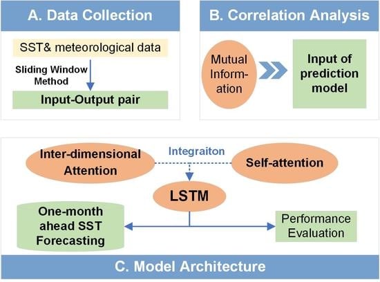
The remainder of this paper is organized as follows. Section 2 first presents the correlation analysis of SST and meteorological data based on mutual information, and then describes the proposed model combining LSTM with attention mechanism. The study area and data sets used, implementation detail, and experimental results are introduced in Section 3. Validation of the model and comparison of its performance with other models are presented in Section 4. Finally, Section 5 concludes this paper and outlines future plans.

2. Methodology

The ocean is a comprehensive and complex dynamic system, and many factors affect the distribution and variation of SST. In the process of multivariate time-series model building, when the dimensionality of the input variables increases to a certain degree, the accuracy of parameter estimation decreases, which significantly decreases the prediction accuracy of the model and generates a dimensional disaster. In addition, the number of learning samples required for training increases exponentially with the dimensionality, whereas in practice the samples available for training are often very limited. By contrast, the model input with an excessive number of irrelevant, redundant, or useless variables, tends to obscure the role of the important variables eventually leading to poor prediction results [35].

Therefore, to identify valid inputs for SST prediction models based on deep learning, it is necessary to analyze the correlation between SST and meteorological and marine factors that may affect SST distribution and variation. On the one hand, by analyzing the correlation between input variables and output variables, the relevant variables that contribute most to the model prediction can be identified. On the other hand, by analyzing whether there is some type of dependency between the input variables, redundant variables can be eliminated.

The present study involves the overall research plan shown in Figure 1. First, we used reanalysis data to construct a database of marine environmental elements, including SST, pressure, wind speed, solar irradiation, latitude, and longitude. Then, we perform quality analysis and corresponding preprocessing according to the analysis result. Because SST is affected by several factors simultaneously, to build a deep learning model, we determine the effective input of the model by analyzing the correlation among the influencing factors based on mutual information. Then, a hybrid model combining LSTM and attention mechanism is introduced. Subsequently, we evaluate the accuracy of the model for the surrounding sea areas of China.

2.1. Correlation Analysis

In general, correlation is used to describe the closeness of the relationship between variables. Correlations include asymmetric causal and driving relationships, as well as symmetric correlations. Among the traditional statistical methods, the Pearson correlation coefficient, Spearman correlation coefficient, and Kendall correlation coefficient are commonly utilized [35]. The Pearson correlation coefficient is used to measure the degree of linear correlation between two variables and requires the corresponding variables to be bivariate normally distributed. The Spearman correlation coefficient is used to analyze a linear correlation using the rank order of two variables; it does not require the distribution of the original variables and is a nonparametric statistical method [36]. The Kendall correlation coefficient is an indicator used to reflect the correlation of categorical variables and is applicable to the case where both variables are ordered categorically.

Commonly applied methods of correlation analysis of multivariate data include Copula analysis, random forest, XGBoost, and mutual information analysis [37]. The definition of mutual information is derived from the concept of entropy in information theory, which is often also called information entropy or Shannon entropy. Entropy expresses the degree of uncertainty in the values of random variables in a numerical form, thus describing the magnitude of information content of variables.

Based on the definition of probability density of data, mutual information is a widely used method to describe the correlation of variables. This is because there is no special requirement for the distribution of data types, and it can be used for both linear and nonlinear correlation analysis [35].

The information entropy of discrete random variables is defined as

$$H(x)=-{\displaystyle \sum _{i=1}^{N}p}\left(x_i\right)\log \left(p\left(x_i\right)\right)$$

(1)

where N is the number of samples and $p\left(x_i\right)$ is the frequency of $x_i$ in the data sets.

The mutual information of variable X and variable Y is defined as

$$I(X,Y)={\displaystyle \iint p_{XY}}(x,y)\log \frac{p_{XY}(x,y)}{p_X(x)p_Y(y)}\mathrm{d}x\mathrm{d}y$$

(2)

where $p_{XY}(x,y)$ is the joint probability density of X and Y, $p_X(x)$ and $p_Y(y)$ are the marginal probability density of X and Y, respectively.

According to the definition, when two variables X and Y are independent of each other or completely unrelated, their mutual information equals to 0, which implies that there is no jointly owned information between the two variables. When X and Y are highly dependent on each other, the mutual information will be large.

In practical problems, the joint probability density of the variables (X, Y) is usually not known, and the variables X and Y are generally discrete. Therefore, the histogram method is commonly used. It discretizes the values of continuous variables by dividing the bins in the range of variables, putting different values of variables into different bins, then counting their frequencies, and subsequently performing calculation using the formula of discrete information entropy. However, determining the range size of each bin is difficult, and it usually requires repeated calculations to obtain the optimal solution.

Another commonly used method is called k-nearest neighbor estimation, which was first proposed in 1987 [38]. In 2004, the mutual information calculation method for computing two continuous random variables was proposed [39].

$$I^{(1)}(X,Y)=\psi (k)-\langle \psi \left(n_x+1\right)+\psi \left(n_y+1\right)\rangle +\psi (N)$$

(3)

$$I^{(2)}(X,Y)=\psi (k)-1/k-\langle \psi \left(n_x\right)+\psi \left(n_y\right)\rangle +\psi (N)$$

(4)

where $\langle \rangle$ is the mean value symbol and $\psi$ is the Digamma function calculated by the following iterative formula

$$\begin{array}{c}\psi (1)=-0.5772516\\ \psi (x+1)=\psi (x)+1/x\end{array}$$

(5)

The results obtained by the two calculation methods are similar in most cases. However, in general, the first method has smaller statistical errors and larger systematic errors, and the second method is more suitable for the calculation of high-dimensional mutual information quantity.

The calculation time of k-nearest neighbor mutual information estimation mainly depends on the sample size, while it is less affected by the dimensionality of variable. Moreover, in general, the smaller the value of k is, the larger is the statistical error and the smaller is the systematic error. Usually, k is taken as 3.

2.2. Model Architecture

LSTM has been widely used in SST time-series prediction. However, the LSTM network requires a long training time because of the lack of parallelization ability. Further, the degree of effect at different time steps on the prediction result are different and varies dynamically with time. This cannot be handled by using LSTM exclusively. Inspired by the attention mechanism used in natural language processing, we added the attention structure into our model to enable it to automatically focus on important historical moments and important variables.

As Figure 2 shows, the model consists of five components. In addition to the necessary input and output module, a multivariate LSTM module is applied to capture the feature information in the time-series data. Integrating multi-dimensional information itself is difficult, because it is impossible to determine which dimension plays a more important role on the results. In addition, the importance of information tends to fluctuate with the time steps. Therefore, it is crucial to solve the problem reasonably linking multi-dimensional input data together to retain useful data and eliminate interfering data. The coefficient matrix W (green part) is determined in a way similar to positional encoding in the attention mechanism. In the blue part, whether the data are true is questioned. A self-attention approach is used to observe the difference between the true and predicted values of the adjacent data; based on this, the data in the current time step is fine-tuned. The weight of the data in the current time step is adjusted to make it closer to the true value in the next iteration.

2.2.1. Interdimensional Attention Strategy

One of the major advantages of a transformer network is that, for a single isolated data point, it not only mines that data point’s information but also integrates multiple data together through positional encoding to mine the information between data. This approach is most suitable for text processing tasks, where a certain association between contexts exists and words are encoded in a uniform manner. However, single-dimensional time-series prediction tasks cannot be realized through this method. In case of SST prediction, owing to the scarcity of data, specific time-stamped information is often erased and only time-course data are retained as a set of information for any consecutive 12 months, rather than a fixed set of information for each month. The variation trend of the data differs for different starting months, even showing totally opposite trends, as illustrated in Figure 3. Moreover, determining the degree of correlation between the data from January 2010 and January 2011 is difficult. Therefore, positional encoding is not possible with only one-dimensional time-series data.

Note that SST at a specific location can be affected by various factors, including the wind speed, air pressure, and solar radiation, to varying degrees, and the general prediction algorithm, which often uses only the temperature data, has significant limitations. SST at a specific place has an implicit relationship with the meteorological factors with a high probability, which can be described by the following equation

$$T_{pred}=k\cdot T+v\cdot u_{10}+\dots$$

(6)

where the coefficients $k$, $v$, and so on are unknown weight vectors, and their values cannot be directly determined on the basis of experience. The main problem is the possible contradiction and inconsistency of importance between parameters. Moreover, the parameters may vary with time steps. For example, the weight of temperature may be set to 0.8 and that of wind speed to 0.2 in January; however, in February, the temperature weight may become 0.7 and the wind speed weight may change to 0.3. Therefore, their values can only be obtained on the basis of the training of the neural network. For each time step, there is a matrix of corresponding coefficient matrix ($k_i$ $v_i$, …). Each coefficient vector is shown in the following equation.

$$k=\left[k_1,k_2,\cdots k_n\right]$$

(7)

where n is the length of time series. Together, these vector coefficients form the W matrix shown in Figure 2.

In this way, during the network training process, the W matrix gradually reveals the implicit connections between these different dimensional data. This combining of data of different dimensions produces an effect similar to the position encoding matrix in a transformer.

2.2.2. Self-Attention Smoothing Strategy

The adverse effects of inevitable systematic errors (e.g., temperature measurement errors, local temperature anomalies, weather anomalies at the time of temperature measurement, and human causes), can be reduced by requiring each data point to be self-conscious, as illustrated in Figure 4.

As shown in Figure 5, to determine whether it is smooth and fits the simulated curve, we need to calculate the relationship between the data at $T_t$, $T_{t-1}$ and $T_{t+1}$. In specific implementations, the degree of fitting is judged by the difference between the predicted and actual values at the current time step is whether around the difference at the preceding and following time step or not. If it is smooth and fits the curve well enough, then the data are more reliable and the corresponding parameter $k$ or $v$ is increased accordingly (blue circle in Figure 4). If it is not smooth or does not fit the curve well enough (green circle in Figure 4), the data may be abnormal and the corresponding parameter $k$ or $v$ is reduced by a factor of 10%. A suitable value can be found after several training iterations.

2.3. Evaluation Metrics

The performance and reliability of the model are evaluated in terms of the statistics of the coefficient of determination (R²), RMSE, mean absolute error (MAE), and mean average percentage error (MAPE). They are defined as Equations (8)–(11), respectively. Here, $y_i$ represents the true SST values, ${\widehat{y}}_i$ represents the predicted SST values, m is the length of the test data sets, and ${\overline{y}}_i$ is the mean value of the true SST.

$$R^2=1-\frac{{\displaystyle \sum _{i=1}^m{\left({\widehat{y}}_i-y_i\right)}^2}}{{\displaystyle \sum _{i=1}^m{\left({\overline{y}}_i-y_i\right)}^2}}$$

(8)

R² is in the range [0, 1]; 0 indicates that the model is poorly fitted, while 1 indicates that the model is error free. In general, the larger the R² is, the better the model.

$$RMSE=\sqrt{\frac{1}{m}{\displaystyle \sum _{i=1}^m{\left(y_i-{\widehat{y}}_i\right)}^2}}$$

(9)

$$MAE=\frac{1}{m}{\displaystyle \sum _{i=1}^m\left|{\widehat{y}}_i-y_i\right|}$$

(10)

$$MAPE=\frac{100\%}{m}{\displaystyle \sum _{i=1}^m\left|\frac{{\widehat{y}}_i-y_i}{y_i}\right|}$$

(11)

The RMSE, MAE and MAPE range in [0, +∞); 0 indicates that the predicted value exactly matches the true value, and the larger the error, the larger the value.

3. Model Implementation and Experiment Results

3.1. Study Area and Data Sets

The study area focuses on the sea areas around China (Figure 6); the specific locations and representative characteristics are shown in

Table 1. Longitude and latitude range and characteristics of study areas.

ID	Ocean Region	Range		Average Depth (m)	Characteristics
		Longitude (E°)	Latitude (N°)
1	Bohai Sea and North Yellow Sea	119~125	37~41	18	Nearly closed
2	South Yellow Sea	119~125	31~37	44	Semi-closed
3	East China Sea	121~125	29~31	370	Marginal sea
4		119~125	25~29
5	Taiwan Strait	119~121	24~25	60	Narrow strait
6		117~120	22~24
7	South China Sea	106~125	5~21	1212	Open sea area

. The distribution and variation of SST depend on multiple meteorological elements. For example, solar radiation has a heating effect on the sea surface. Wind is the direct driver of the upper ocean circulation, which is an important factor to determine the flow of the upper layer and affects the distribution of SST [19].

This study considers the temporal and spatial resolution of the data and the completeness of the environmental variables fully, then the fifth-generation ECMWF (European Centre for Medium-Range Weather Forecasts) reanalysis (ERA5) is selected to construct a multi-physical field data set of marine environmental elements for the sea areas around China. ERA5 provides hourly, daily and monthly estimates for a large number of atmospheric, ocean-wave and land-surface quantities [40].

The temporal resolution of the data used in this study is monthly and the data sets cover the period 1979–2021. The spatial resolution in latitude and longitude is 0.25°. As illustrated in

Table 2. Variables affecting SST distribution and variation.

Parameters	Name	Unit
SST	Sea surface temperature	K
u10	Eastward component of the 10 m wind	m/s
v10	Northward component of the 10 m wind	m/s
msl	Mean sea level pressure	Pa
ssr	Surface net solar radiation	J/m2
ssrc	Surface net solar radiation clear sky	J/m2
str	Surface net thermal radiation	J/m2
strc	Surface net thermal radiation clear sky	J/m2
ssrd	Surface solar radiation downward	J/m2
ssrdc	Surface solar radiation downward clear sky	J/m2
strd	Surface solar radiation downwards	J/m2
strdc	Surface thermal radiation downward clear sky	J/m2

, in addition to SST data, data on meteorological factors including wind speed, sea surface pressure, and sea surface solar radiation have been collected.

3.2. Implementation Detail

As shown in Table 2, the data sets consist of various parameters that have different units and ranges of values; thus, data normalization is necessary. The min-max normalization is utilized to scale the data between 0 and 1,

$$z_i=\frac{x_i-x_{\min }}{x_{\max }-x_{\min }}$$

(12)

where $x_i$ is the original data, $x_{\min }$ and $x_{\max }$ are the minimum and maximum of the original data, respectively.

Then, to transform the time series into input–output pairs required for model training, a sliding window with a fixed length is used as shown in Figure 7. In this study, the model receives an instance with a sliding window of length 12 as input and performs one-step predictions. The resulting samples are divided into training, validation, and test sets in a ratio of 6:1:2.

As shown in

Table 3. Key parameters of the model and training process.

Key Parameters	Model Methods or Values
Length of training data sets	300
Length of validation data sets	50
Length of testing data sets	100
Architecture of the model	Attention + LSTM + Dense
Input dimension	12 × 4
Output dimension	1
No. of neural of hidden layer	80
Optimizer	Adam
Epoch	400
Batch size	40
Dropout	0.1
Loss function	RMSE

, the training rate is improved by using a batch training method, with each batch containing 40 sample data sets. In addition, a random dropout layer is added after each layer of the LSTM network with a dropout rate setting as 0.1 to avoid overfitting. Next, the root mean squared error (RMSE) is chosen as the loss function for training, and the Adam algorithm is used to train the network. The number of maximum iterations (epoch) is set to 400.

All experiments are implemented using Keras 2.2.4 with TensorFlow 1.15.0 on a computer with an Intel i9-10900K CPU and an additional NVIDIA GeForce RTX 2080S GPU.

3.3. Experiment Results

3.3.1. SST Distribution and Variation

From Figure 8, Figure 9 and Figure 10, it can be concluded that the latitudinal distribution of SST is obvious, i.e., the South China Sea has a lower latitude and a higher temperature all year round. The annual variation, except for the South China Sea, shows a pattern of synchronous change with the temperature, i.e., the highest in August and the lowest in January.

3.3.2. Correlation of SST with Other Meteorological Factors

In this study, mutual information is selected as a tool to analyze the correlations between different environmental factors and SST, which is further required for selecting the effective input variable for building a deep learning prediction model.

The mutual information of SST with each influencing factor was calculated using k-nearest neighbor-based mutual information, as shown in Figure 11. The figure indicates that, overall, the wind speed (u10, v10) and air pressure at sea level (msl) correlate more strongly with SST in different seas compared to radiation-related environmental variables.

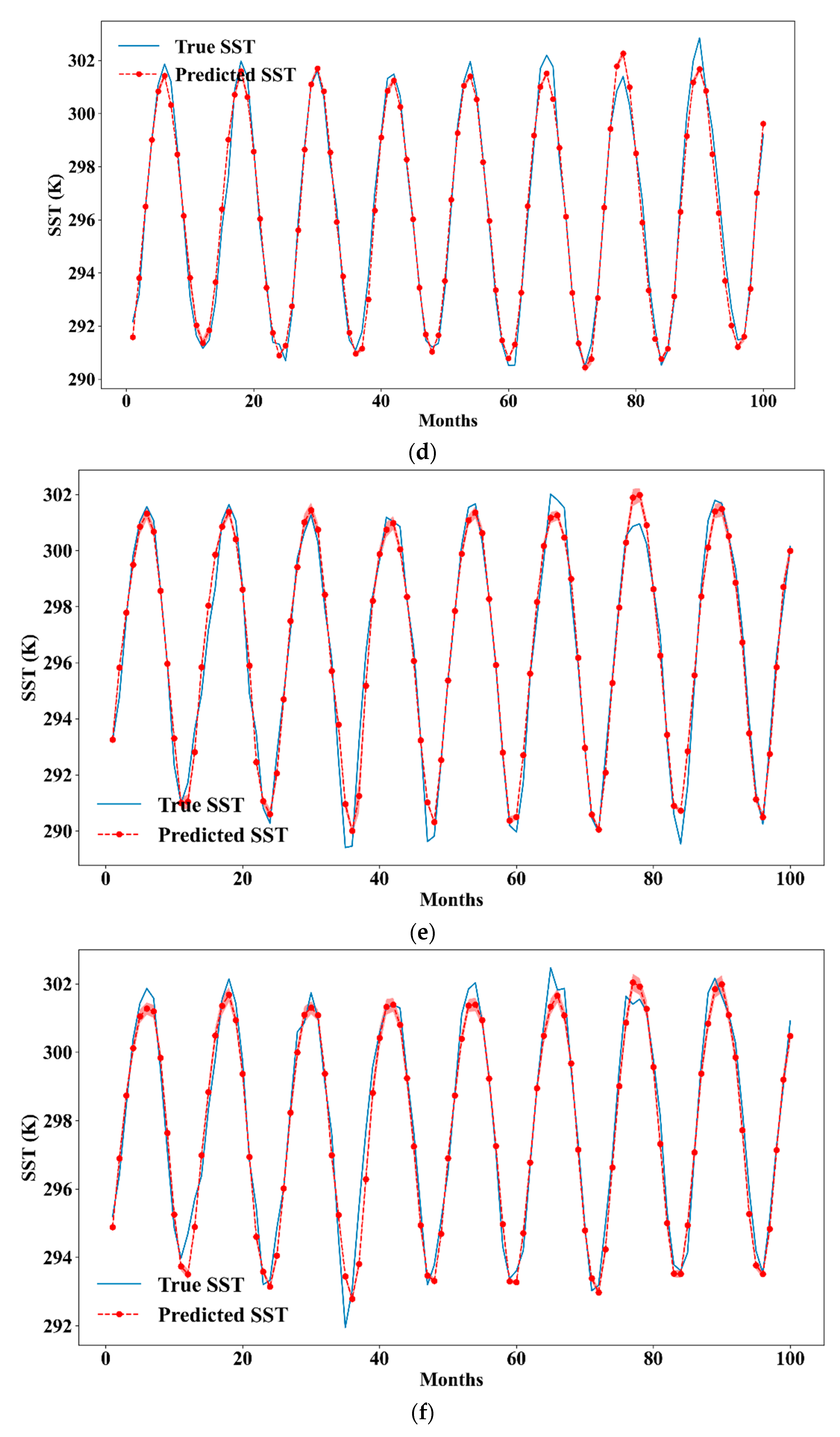
3.3.3. SST Prediction Results

The last 100 samples (about 8 years from 2014 to 2021) in the data sets are applied to test the model. The one-month ahead monthly mean SST prediction results of the sea areas around China are shown in Figure 12. The blue line represents the true values. Additionally, the red dot and the filled areas in the figure represent the average prediction results and the corresponding standard deviation for five runs. What should be noted is that the resolution of y axis is different for different regions.

Overall, the prediction results reveal a same trend between the true and predicted SST. However, for all regions, larger bias appears at the local extremums, because the model trained on the training data sets cannot capture the extremums of the test data sets. As SST of southern part of China, especially South China Sea, keeps high (approximately 300 K) all year round and fluctuates less, the model performs better.

To test the stability of the model, statistics including R², RMSE, MAE, and MAPE for five runs are presented in

Table 4. Comparison of R², RMSE, MAE and MAPE for seven study areas (average for five runs).

Region ID	R2	RMSE	MAE	MAPE
1	0.9910	0.7551	0.6211	0.2170
2	0.9829	0.8789	0.6803	0.2336
3	0.9827	0.7547	0.5936	0.2029
4	0.9827	0.5120	0.4100	0.1382
5	0.9727	0.6515	0.5065	0.1711
6	0.9649	0.5666	0.4531	0.1521
7	0.9138	0.3928	0.3213	0.1067

and Figure 13. From the perspective of RMSE, MAE and MAPE, the model performs better in the southern parts of the surrounding seas of China, especially the South China Sea, for which the SST varies less and maintains a high value all year round. The error of some isolated point probably leads to higher RMSE, MAE and MAPE. The fluctuation for region 5 (Taiwan Strait) is the smallest, which may indicate that, for narrow strait areas, we can trust the result more from arbitrary initialization conditions.

4. Discussion

4.1. Performance Comparison with Other Models

Table 5. Comparison of RMSE between different models.

Region ID	LSTM Only with SST Only as Input	LSTM Only	Our Model
1	1.0157	0.9226	0.7551
2	1.0302	0.8657	0.8789
3	1.0481	0.7853	0.7547
4	0.8388	0.7301	0.5120
5	1.2139	0.8768	0.6515
6	0.7678	0.6487	0.5666
7	0.4140	0.4018	0.3928

shows the performance comparison of two other models with the model considering attention mechanism and taking both SST and meteorological factors as inputs. One of the models is the LSTM model taking SST only as input, and the other model takes SST and meteorological factors as inputs without considering attention mechanism. The boldface items in the table represent the best performance. The hyper-parameters affecting the training process are the same for the models.

It can be seen from the results that our model achieves the best performance for most regions. For the South China sea areas, three models show similar performance. Thus, it enables researchers to use the simple LSTM-only model with SST only as input for predicting SST in southern regions of China when there are insufficient meteorological data or computing resources.

4.2. Overfitting Issue Varification

To test if the trained model has overfitting issue, we have done another experiment to validate the generalization capability of the model. The forty-three-year (1979–2021) monthly mean SST and meteorological time-series data from ERA5 are used to train and validate the model. Then, the eight-year (1971–1978) data sets are fed into the trained model.

The prediction results shown in Figure 14 are the average for five runs, which verify the applicability and effectiveness of model. The black and red line represent the true values average prediction results.

5. Conclusions

SST is a significant physical parameter used in the analysis of the ocean and climate. This study developed a data-driven model for predicting one-month ahead monthly mean SST by combining interdimensional and self-attention mechanism with neural networks. After correlation analysis by mutual information, SST and other meteorological factors including wind speed and air pressure were selected as the input of the prediction model. The interdimensional attention enabled the model to focus on important historical moments and important variables while the self-attention mechanism was utilized to smooth the data in the training process. Forty-three-year monthly mean SST and meteorological time-series data from ERA5 of ECMWF were collected to train the model and test its performance for the sea areas around China. The evaluation criteria of R², RMSE, MAE and MAPE indicate that the predicted results met the requirement for oceanography and meteorology studies.

During experiment, we find that, in most cases, other meteorological factors contribute to the predicted results, but these data, especially the wind speed, are not as stable as SST data and are prone to anomalies. The model is unable to reduce its coefficients quickly enough, thus leading to a longer training process eventually

Overall, the performance of the model on SST prediction is promising. Future work involves further optimization of the model and investigation of its applicability for other ocean physical parameters such as sea surface salinity, and ocean water temperature underneath the surface.

References

1. O’carroll, A.G.; Armstrong, E.M.; Beggs, H.M.; Bouali, M.; Casey, K.S.; Corlett, G.K.; Dash, P.; Donlon, C.L.; Gentemann, C.L.; Høyer, J.L.; et al. Observational Needs of Sea Surface Temperature. Front. Mar. Sci. 2019, 6, 1–27. [Google Scholar] [CrossRef]
2. Kim, M.; Yang, H.; Kim, J. Sea Surface Temperature and High Water Temperature Occurrence Prediction Using a Long Short-Term Memory Model. Remote Sens. 2020, 12, 3654–3674. [Google Scholar] [CrossRef]
3. Baoleerqimuge, R.G.Y. Sea Surface Temperature Observation Methods and Comparison of Commonly Used Sea Surface Temperature Datasets. Adv. Meteorol. Sci. Technol. 2013, 3, 52–57. [Google Scholar] [CrossRef]
4. Hou, X.Y.; Guo, Z.H.; Cui, Y.K. Marine big data: Concept, applications and platform construction. Bull. Mar. Sci. 2017, 36, 361–369. [Google Scholar] [CrossRef]
5. Jiang, X.W.; Xi, M.; Song, Q.T. A Comparison of Six Sea Surface Temperature Analyses. Acta Oceanol. Sin. 2013, 35, 88–97. [Google Scholar] [CrossRef]
6. Wang, C.Q.; Li, X.; Zhang, Y.F.; Zu, Z.Q.; Zhang, R.Y. A comparative study of three SST reanalysis products and buoys data over the China offshore area. Acta Oceanol. Sin. 2020, 42, 118–128. [Google Scholar] [CrossRef]
7. Sarkar, P.P.; Janardhan, P.; Roy, P. Prediction of sea surface temperatures using deep learning neural networks. SN Appl. Sci. 2020, 2, 1458. [Google Scholar] [CrossRef]
8. Wolff, S.; O’Donncha, F.; Chen, B. Statistical and machine learning ensemble modelling to forecast sea surface temperature. J. Mar. Syst. 2020, 208, 103347. [Google Scholar] [CrossRef]
9. LeCun, Y.; Bengio, Y.; Hinton, G. Deep learning. Nature 2015, 521, 436–444. [Google Scholar] [CrossRef]
10. Lins, I.D.; Araujo, M.; das Chagas Moura, M.; Silva, M.A.; Droguett, E.L. Prediction of sea surface temperature in the tropical Atlantic by support vector machines. Comput. Stat. Data Anal. 2013, 61, 187–198. [Google Scholar] [CrossRef]
11. Li, W.; Lei, G.; Qu, L.Q. Prediction of sea surface temperature in the South China Sea by artificial neural networks. IEEE Geosci. Remote. Sens. Lett. 2020, 17, 558–562. [Google Scholar] [CrossRef]
12. Zhu, L.Q.; Liu, Q.; Liu, X.D.; Zhang, Y.H. RSST-ARGM: A data-driven approach to long-term sea surface temperature prediction. J. Wirel. Commun. Netw. 2021, 2021, 171. [Google Scholar] [CrossRef]
13. Hinton, G.E.; Osindero, S.; Teh, Y.W. A fast learning algorithm for deep belief nets. Neural Comput. 2006, 18, 1527–1554. [Google Scholar] [CrossRef]
14. Qiu, X.P. Neural Networks and Deep Learning; China Machine Press: Beijing, China, 2020; pp. 139–141. [Google Scholar]
15. Hochreiter, S.; Schmidhuber, J. Long short-term memory. Neural Comput. 1997, 9, 1735–1780. [Google Scholar] [CrossRef]
16. Shi, X.J.; Chen, Z.R.; Wang, H.; Yeung, D.Y.; Wong, W.K.; Woo, W.C. Convolutional LSTM Network: A Machine Learning Approach for Precipitation Nowcasting. In Proceedings of the International Conference on Neural Information Processing Systems, Montreal, QC, Canada, 7–12 December 2015; pp. 802–810. [Google Scholar]
17. Xu, B.N.; Jiang, J.R.; Hao, H.Q.; Lin, P.F.; He, D.D. A Deep Learning Model of ENSO Prediction Based on Regional Sea Surface Temperature Anomaly Prediction. Electron. Sci. Technol. Appl. 2017, 8, 65–76. [Google Scholar] [CrossRef]
18. Yang, Y.; Dong, J.; Sun, X.; Lima, E.; Mu, Q.; Wang, X. A CFCC-LSTM model for sea surface temperature prediction. IEEE Geosci. Remote. Sens. Lett. 2018, 15, 207–211. [Google Scholar] [CrossRef]
19. Zhu, G.C.; Hu, S. Study on sea surface temperature model based on LSTM-RNN. J Appl. Oceanogr. 2019, 38, 191–197. [Google Scholar] [CrossRef]
20. Sun, T.; Feng, Y.; Li, C.; Zhang, X. High Precision Sea Surface Temperature Prediction of Long Period and Large Area in the Indian Ocean Based on the Temporal Convolutional Network and Internet of Things. Sensors 2022, 22, 1636. [Google Scholar] [CrossRef] [PubMed]
21. Aydınlı, H.O.; Ekincek, A.; Aykanat-Atay, M.; Sarıtaş, B.; Özenen-Kavlak, M. Sea surface temperature prediction model for the Black Sea by employing time-series satellite data: A machine learning approach. Appl. Geomat. 2022, 1–10. [Google Scholar] [CrossRef]
22. Patil, K.; Deo, M.; Ravichandran, M. Prediction of sea surface temperature by combining numerical and neural techniques. J. Atmos. Ocean. Technol. 2016, 33, 1715–1726. [Google Scholar] [CrossRef]
23. Xiao, C.; Chen, N.; Hu, C.; Wang, K.; Chen, Z. Short and mid-term sea surface temperature prediction using time-series satellite data and LSTM-AdaBoost combination approach. Remote Sens. Environ. 2019, 233, 111358. [Google Scholar] [CrossRef]
24. Xiao, C.; Chen, N.; Hu, C.; Wang, K.; Xu, Z.; Cai, Y.; Xu, L.; Chen, Z.; Gong, J. A spatiotemporal deep learning model for sea surface temperature field prediction using time-series satellite data. Environ. Model Softw. 2019, 120, 104502. [Google Scholar] [CrossRef]
25. He, Q.; Cha, C.; Song, W.; Hao, Z.Z.; Huang, D.M. Sea surface temperature prediction algorithm based on STL model. Mar. Environ. Sci. 2020, 39, 104–111. [Google Scholar] [CrossRef]
26. de Mattos Neto, P.S.G.; Cavalcanti, G.D.C.; de, O.S.J.D.S.; Silva, E.G. Hybrid Systems Using Residual Modeling for Sea Surface Temperature Forecasting. Sci. Rep. 2022, 12, 487. [Google Scholar] [CrossRef]
27. Jahanbakht, M.; Xiang, W.; Azghadi, M.R. Sea Surface Temperature Forecasting With Ensemble of Stacked Deep Neural Networks. IEEE Geosci. Remote. Sens. Lett. 2022, 19, 1–5. [Google Scholar] [CrossRef]
28. Liu, X.; Li, N.; Guo, J.; Fan, Z.; Lu, X.; Liu, W.; Liu, B. Multi-step-ahead Prediction of Ocean SSTA Based on Hybrid Empirical Mode Decomposition and Gated Recurrent Unit Model. IEEE J. Sel. Top. Appl. Earth Obs. Remote Sens. 2022, 15, 7525–7538. [Google Scholar] [CrossRef]
29. Lara-Benítez, P.; Carranza-García, M.; Riquelme, J.C. An experimental review on deep learning architectures for time series forecasting. Int. J. Neural Syst. 2021, 31, 2130001. [Google Scholar] [CrossRef]
30. Vaswani, A.; Shazeer, N.; Parmar, N.; Uszkoreit, J.; Jones, L.; Gomez, A.N.; Kaiser, Ł.; Polosukhin, I. Attention is all you need. arXiv 2017. [Google Scholar] [CrossRef]
31. Li, S.; Jin, X.; Xuan, Y.; Zhou, X.; Chen, W.; Wang, Y.-X.; Yan, X. Enhancing the locality and breaking the memory bottleneck of transformer on time series forecasting. In Proceedings of the Conference on Neural Information Processing Systems, Vancouver, BC, Canada, 8–14 December 2019; pp. 1–11. [Google Scholar]
32. Xie, J.; Zhang, J.; Yu, J.; Xu, L. An adaptive scale sea surface temperature predicting method based on deep learning with attention mechanism. IEEE Geosci. Remote. Sens. Lett. 2019, 17, 740–744. [Google Scholar] [CrossRef]
33. Mohammadi Farsani, R.; Pazouki, E. A transformer self-attention model for time series forecasting. J. Electr. Comput. Eng. Innov. 2021, 9, 1–10. [Google Scholar] [CrossRef]
34. Xu, W.X.; Shen, Y.D. Bus travel time prediction based on Attention-LSTM neural network. Mod. Electron. Technol. 2022, 45, 83–87. [Google Scholar] [CrossRef]
35. Liu, X.X. Correlation Analysis and Variable Selection for multivariateTime Series based a on Mutual Informationerles. Master’s Thesis, Dalian University of technology, Dalian, China, 2013. [Google Scholar]
36. De Winter, J.C.; Gosling, S.D.; Potter, J. Comparing the Pearson and Spearman correlation coefficients across distributions and sample sizes: A tutorial using simulations and empirical data. Psychol. Methods 2016, 21, 273–290. [Google Scholar] [CrossRef]
37. Li, G.J. Research on Time Series Forecasting Based on Multivariate Analysis. Master’s Thesis, Tianjin University of Technology, Tianjin, China, 2021. [Google Scholar]
38. Kozachenko, L.F.; Leonenko, N.N. Sample estimate of the entropy of a random vector. Probl. Inf. Transm. 1987, 23, 9–16. [Google Scholar]
39. Kraskov, A.; Stögbauer, H.; Grassberger, P. Estimating mutual information. Phys. Rev. E 2004, 69, 66138. [Google Scholar] [CrossRef]
40. Hersbach, H.; Bell, B.; Berrisford, P.; Biavati, G.; Horányi, A.; Muñoz Sabater, J.; Nicolas, J.; Peubey, C.; Radu, R.; Rozum, I.; et al. ERA5 monthly averaged data on single levels from 1959 to present. Copernic. Clim. Change Serv. (C3S) Clim. Data Store (CDS) 2019, 10, 252–266. [Google Scholar] [CrossRef]
Figure 1. General flow chart of SST prediction based on a hybrid model combining LSTM and attention.
Remotesensing 14 04737 g001
Figure 2. Structural diagram of the attention-based LSTM model.
Remotesensing 14 04737 g002
Figure 3. Variation trend of SST in a sliding window.
Remotesensing 14 04737 g003
Figure 4. Self-attention smoothing strategy.
Remotesensing 14 04737 g004
Figure 5. Specific execution process of self-attention smoothing.
Remotesensing 14 04737 g005
Figure 6. Location of the seven sea areas around China.
Remotesensing 14 04737 g006
Figure 7. Sliding window procedure to obtain input–output pair of data sets.
Remotesensing 14 04737 g007
Figure 8. SST distribution of sea areas surrounding China in (a) March, (b) June, (c) September, and (d) December in 2021.
Remotesensing 14 04737 g008
Figure 9. Variation of monthly mean SST for different sea areas around China during 1979–2021.
Remotesensing 14 04737 g009
Figure 10. Statistics of monthly mean SST including minimum, maximum, and mean value for different parts of China’s Surrounding Seas during 1979–2021.
Remotesensing 14 04737 g010
Figure 11. Heat map of mutual information for each meteorological variable and SST for the seas around China in different months (a) Bohai Sea and north part of Yellow Sea, (b) South part of Yellow Sea, (c) Part 1 (ID:3 in Table 1) of East China Sea, (d) Part 2 (ID:4 in Table 1) of East China Sea, (e) Part 1(ID:5 in Table 1) of Taiwan Strait, (f) Part 2(ID:5 in Table 1) of Taiwan Strait, and (g) South China Sea.
Remotesensing 14 04737 g011aRemotesensing 14 04737 g011b
Figure 12. SST prediction results of the sea areas around China (a) Bohai Sea and north part of Yellow Sea, (b) South part of Yellow Sea, (c) Part 1 (ID:3 in Table 1) of East China Sea, (d) Part 2 (ID:4 in Table 1) of East China Sea, (e) Part 1(ID:5 in Table 1) of Taiwan Strait, (f) Part 2(ID:5 in Table 1) of Taiwan Strait and (g) South China Sea.
Remotesensing 14 04737 g012aRemotesensing 14 04737 g012bRemotesensing 14 04737 g012c
Figure 13. The distribution of the evaluation index for five runs: (a) RMSE, (b) R-squared, (c) MAE and (d) MAPE.
Remotesensing 14 04737 g013
Figure 14. Evaluation of the generalization ability of the model. (a) Bohai Sea and north part of Yellow Sea, (b) South part of Yellow Sea, (c) Part 1 (ID:3 in Table 1) of East China Sea, (d) Part 2 (ID:4 in Table 1) of East China Sea, (e) Part 1(ID:5 in Table 1) of Tai-wan Strait, (f) Part 2(ID:5 in Table 1) of Taiwan Strait and (g) South China Sea.
Remotesensing 14 04737 g014aRemotesensing 14 04737 g014bRemotesensing 14 04737 g014c