
Using GEOBIA and Vegetation Indices to Assess Small Urban Green Areas in Two Climatic Regions

 , , , ,
  , and
, and 
Abstract
:
1. Introduction
- (1)
- to determine whether small urban green areas can be extracted by applying GEOBIA to Planet timeseries in two different biogeographical and climatic regions;
- (2)
- to compare the quality of small urban green areas in two different biogeographical and climatic regions.
2. Data and Methodology
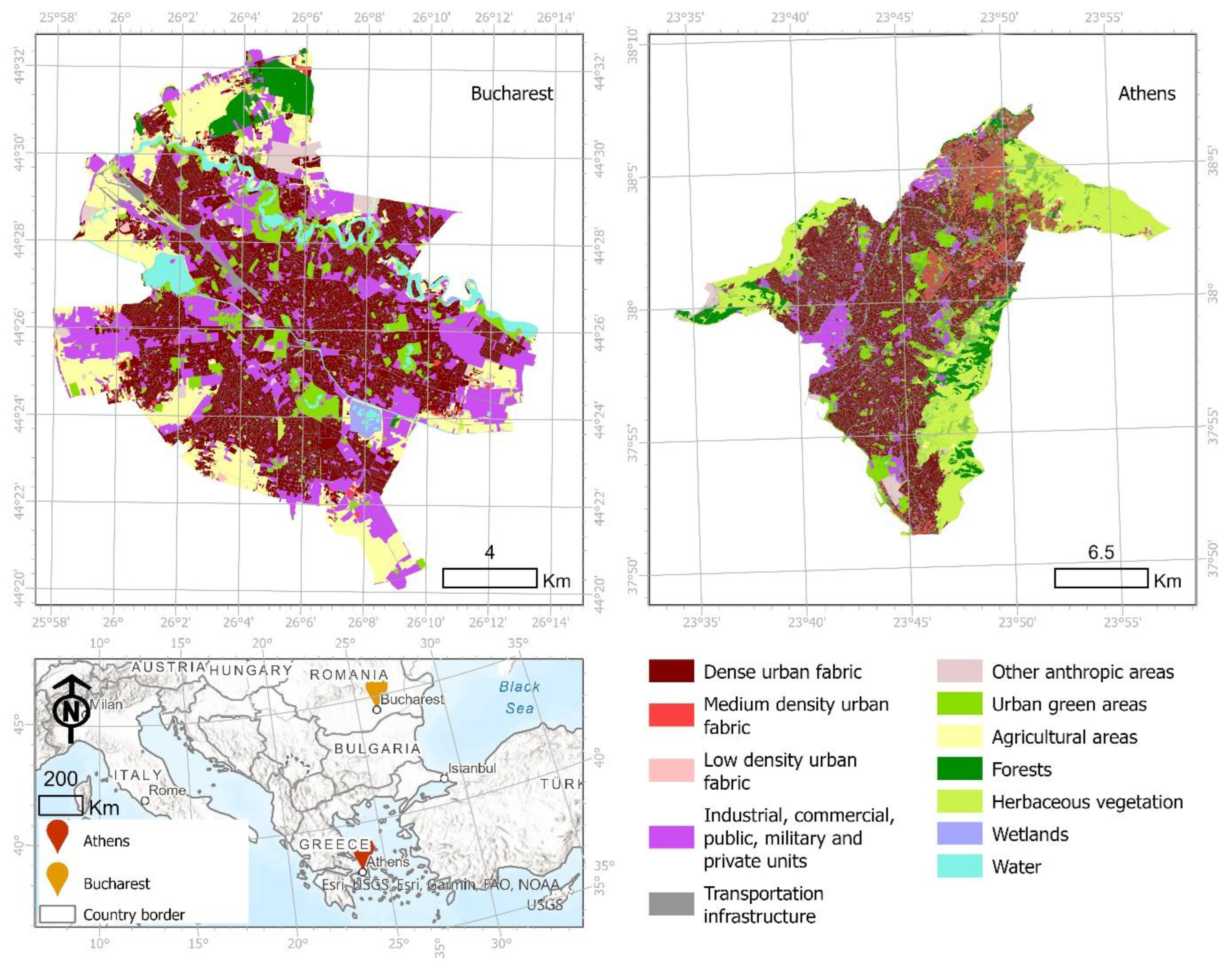
2.1. Study Area
2.2. Extracting Small Urban Green Areas Using GEOBIA
2.3. Vegetation Indices Used for Assessing the Quality of Small Urban Green Areas

| Index Code | Index | Formula |
|---|---|---|
| MSAVI2 | Modified Soil Adjusted Vegetation Index 2 | |
| NDVI | Normalized Difference Vegetation Index |
2.4. Factors Influencing the Quality of Small Urban Green Spaces
3. Results
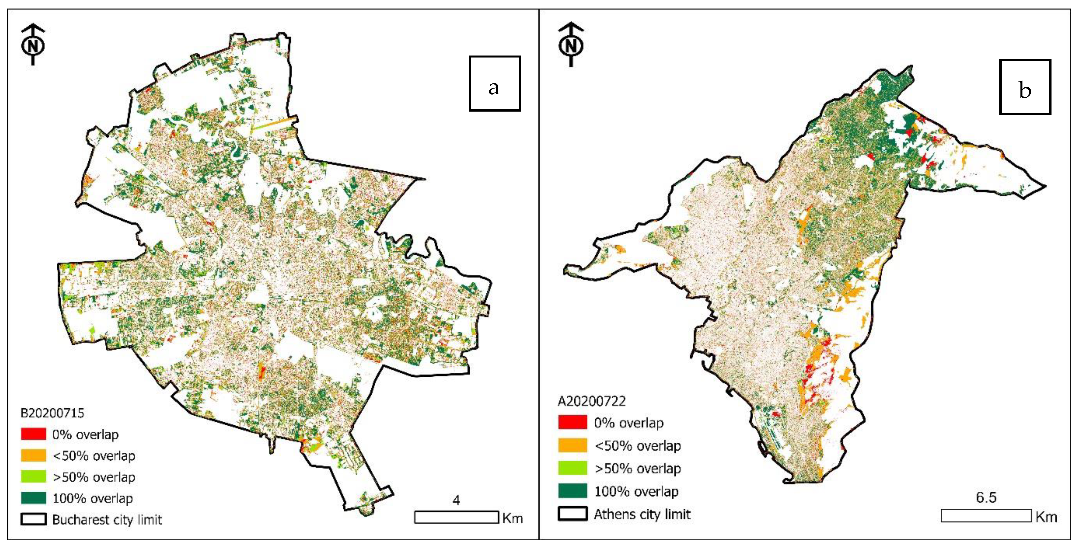
3.1. Distribution and Dynamics of Small Urban Green Areas
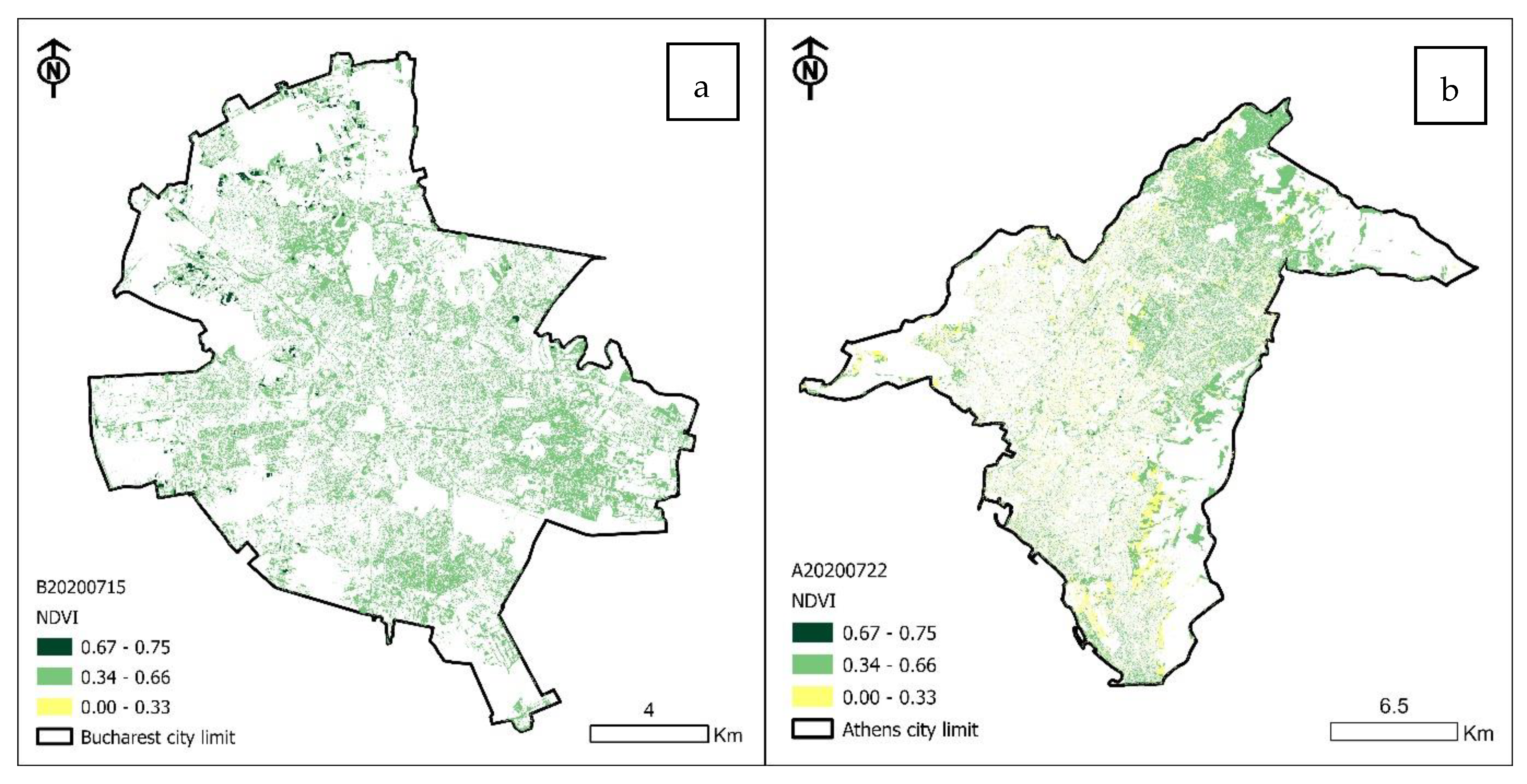
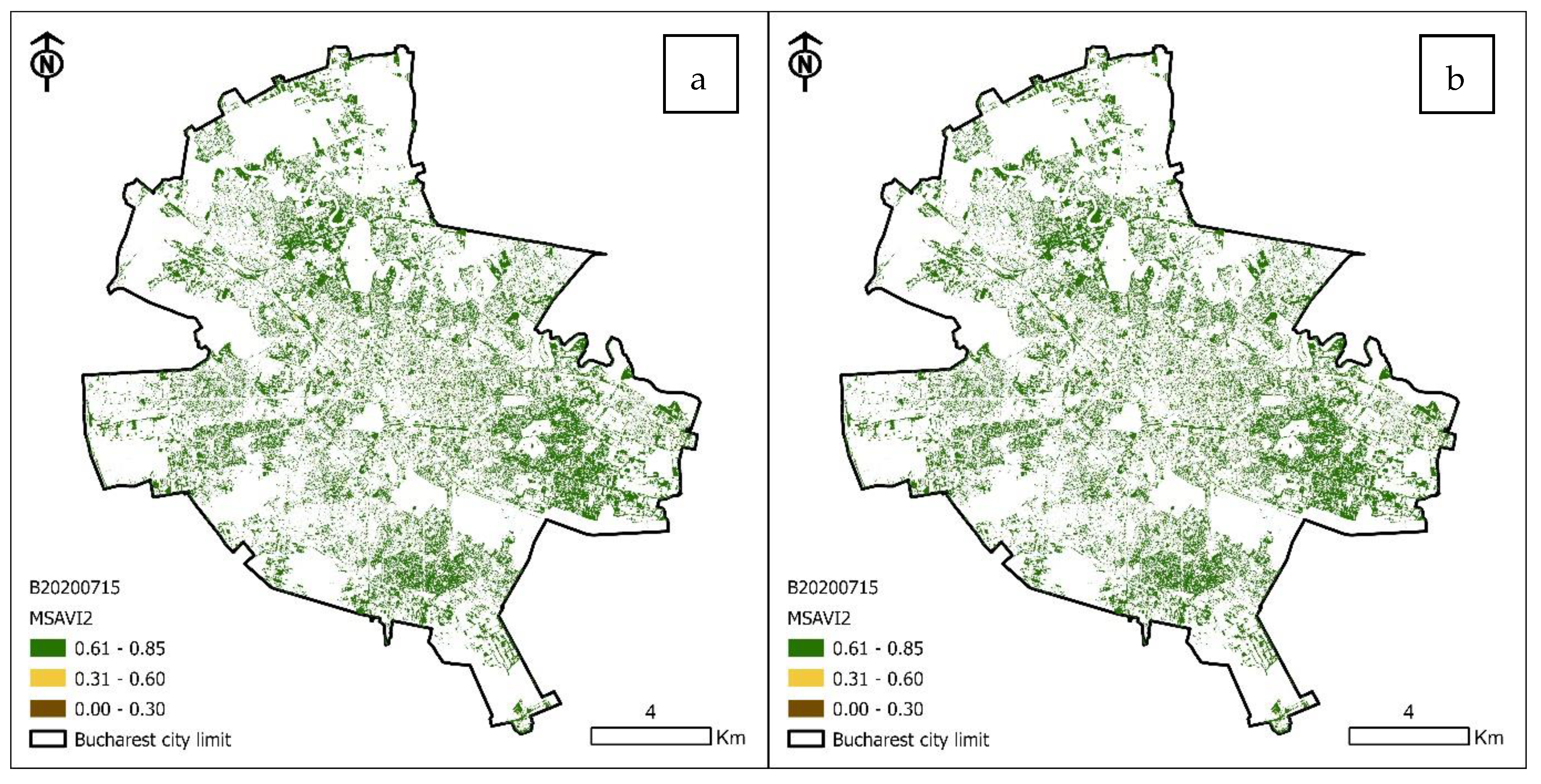
3.2. Quality of Small Urban Green Areas
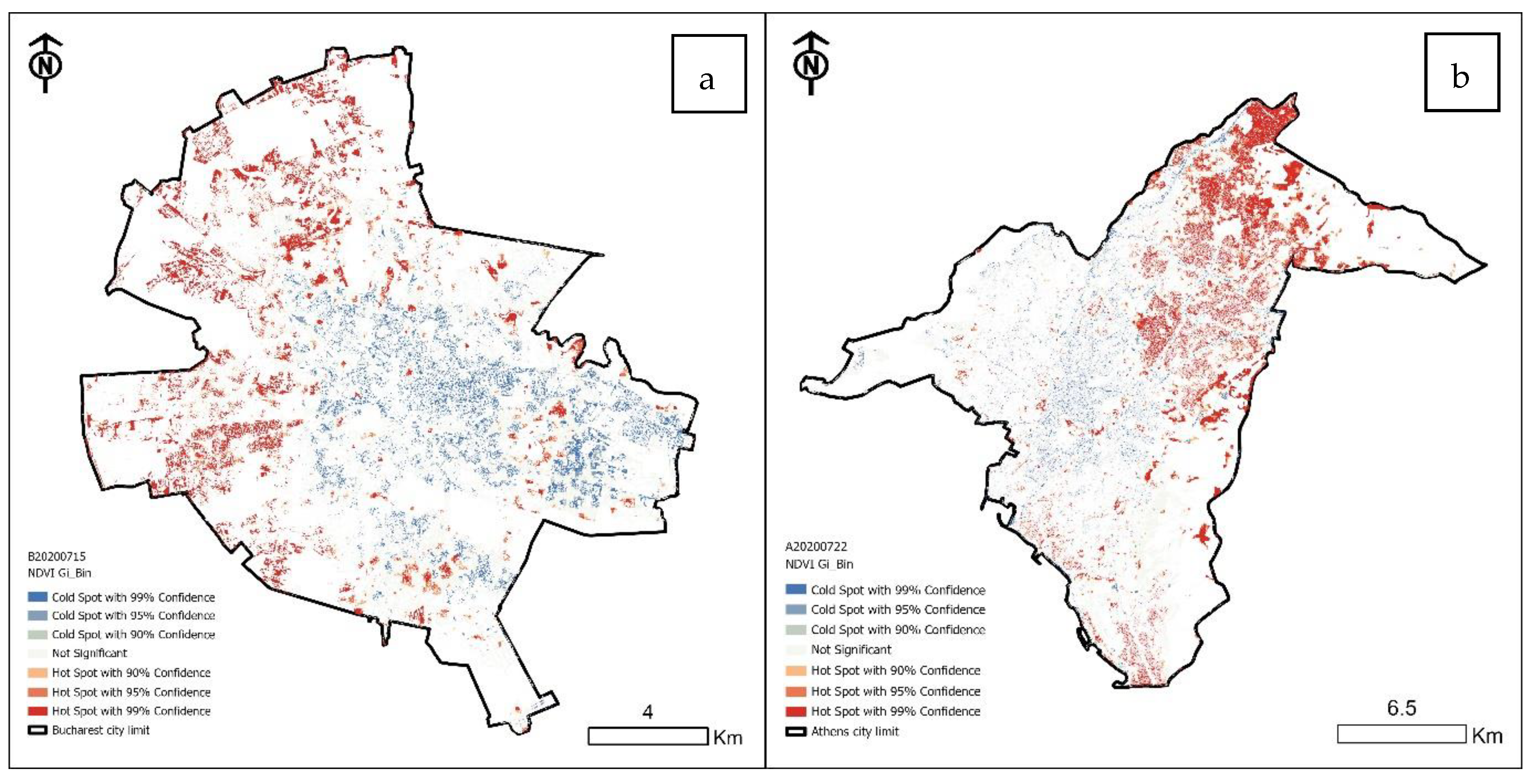
3.3. Spatial Distribution of the Quality of Small Urban Green Areas
4. Discussions
4.1. Method’s Efficiency for Extracting Small Urban Green Areas
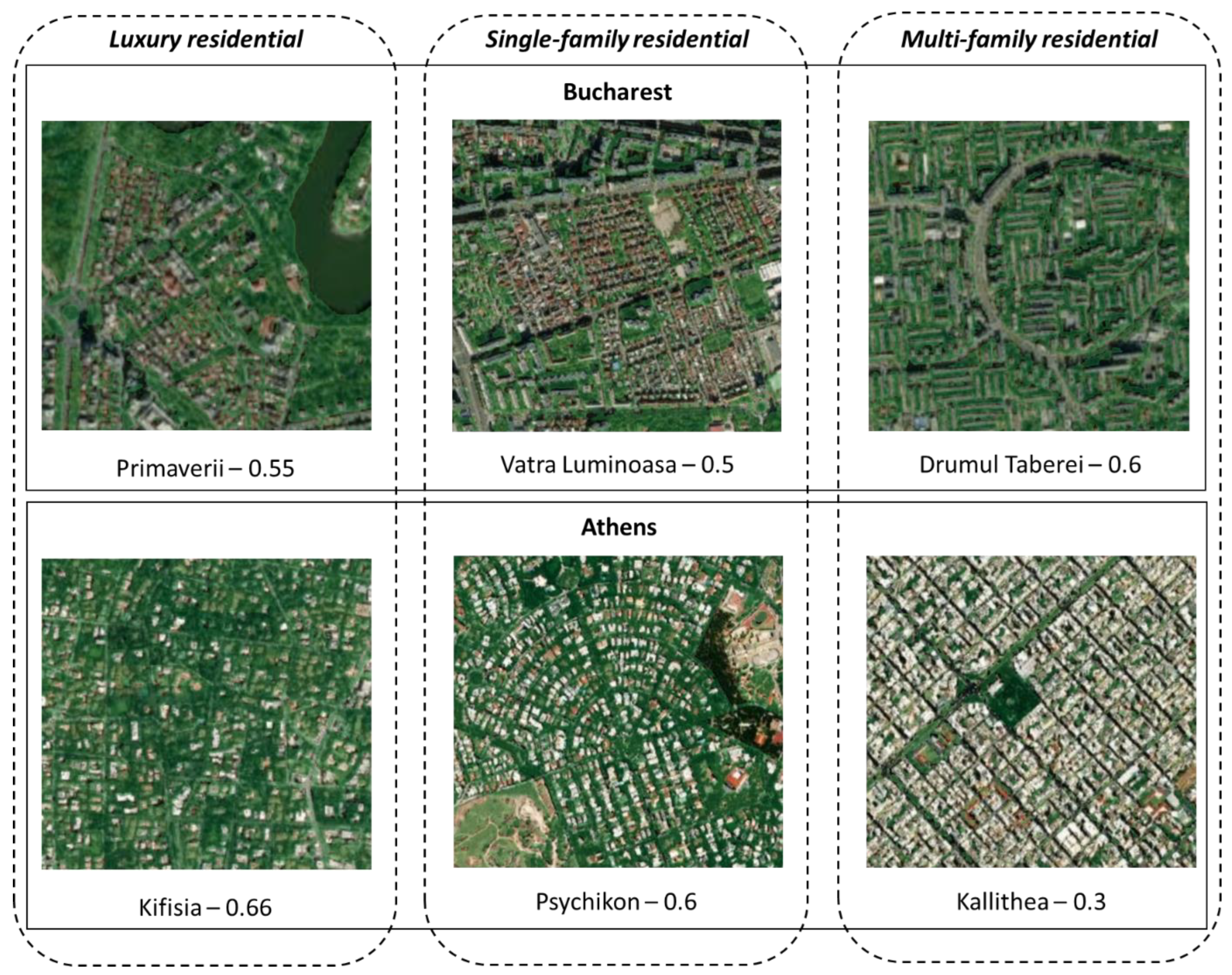
4.2. Insights into the Quality of Small Urban Green Areas
4.3. Influence of Climatic and Biogeographical Characteristics
5. Conclusions
Author Contributions
Funding
Acknowledgments
Conflicts of Interest
References
- United Nations. Habitat III New Urban Agenda; United Nations: New York, NY, USA, 2017. [Google Scholar]
- United Nations Sustainable Development Goals. Available online: https://sustainabledevelopment.un.org/index.php?menu=1300 (accessed on 16 May 2019).
- Bush, J.; Doyon, A. Building Urban Resilience with Nature-Based Solutions: How Can Urban Planning Contribute? Cities 2019, 95, 102483. [Google Scholar] [CrossRef]
- United for Smart Sustainable Cities. Implementing Sustainable Development Goal 11 by Connecting Sustainability Policies and Urban-Planning Practices through ICTs; United Nations: New York, NY, USA, 2017. [Google Scholar]
- Peschardt, K.K.; Schipperijn, J.; Stigsdotter, U.K. Use of Small Public Urban Green Spaces (SPUGS). Urban For. Urban Green. 2012, 11, 235–244. [Google Scholar] [CrossRef]
- Popa, A.-M.; Ioja, I.-C.; Nita, M.-R.; Onose, D.-A. Urban Sustainability Assessment of Romanian Cities. Carpathian J. Earth Environ. Sci. 2022, 17, 373–385. [Google Scholar]
- Huang, Y.; Lin, T.; Zhang, G.; Jones, L.; Xue, X.; Ye, H.; Liu, Y. Spatiotemporal Patterns and Inequity of Urban Green Space Accessibility and Its Relationship with Urban Spatial Expansion in China during Rapid Urbanization Period. Sci. Total Environ. 2022, 809, 151123. [Google Scholar] [CrossRef] [PubMed]
- Siddique, S.; Uddin, M.M. Green Space Dynamics in Response to Rapid Urbanization: Patterns, Transformations and Topographic Influence in Chattogram City, Bangladesh. Land Use Policy 2022, 114, 105974. [Google Scholar] [CrossRef]
- Picard, P.M.; Tran, T.T.H. Small Urban Green Areas. J. Environ. Econ. Manag. 2021, 106, 102418. [Google Scholar] [CrossRef]
- Naghibi, M.; Faizi, M.; Ekhlassi, A. Design Possibilities of Leftover Spaces as a Pocket Park in Relation to Planting Enclosure. Urban For. Urban Green. 2021, 64, 127273. [Google Scholar] [CrossRef]
- Zhang, X.; Ni, Z.; Wang, Y.; Chen, S.; Xia, B. Public Perception and Preferences of Small Urban Green Infrastructures: A Case Study in Guangzhou, China. Urban For. Urban Green. 2020, 53, 126700. [Google Scholar] [CrossRef]
- Parlamentul Romaniei. Legea 24/2007; Parlamentul Romaniei: Bucharest, Romania, 2012. [Google Scholar]
- Nordh, H.; Østby, K. Pocket Parks for People—A Study of Park Design and Use. Urban For. Urban Green. 2013, 12, 12–17. [Google Scholar] [CrossRef]
- Park, J.; Kim, J.H.; Lee, D.K.; Park, C.Y.; Jeong, S.G. The Influence of Small Green Space Type and Structure at the Street Level on Urban Heat Island Mitigation. Urban For. Urban Green. 2017, 21, 203–212. [Google Scholar] [CrossRef]
- Strohbach, M.W.; Lerman, S.B.; Warren, P.S. Are Small Greening Areas Enhancing Bird Diversity? Insights from Community-Driven Greening Projects in Boston. Landsc. Urban Plan. 2013, 114, 69–79. [Google Scholar] [CrossRef]
- Lin, W.; Chen, Q.; Jiang, M.; Zhang, X.; Liu, Z.; Tao, J.; Wu, L.; Xu, S.; Kang, Y.; Zeng, Q. The Effect of Green Space Behaviour and per Capita Area in Small Urban Green Spaces on Psychophysiological Responses. Landsc. Urban Plan. 2019, 192, 103637. [Google Scholar] [CrossRef]
- Kolokotsa, D.; Lilli, A.; Lilli, M.A.; Nikolaidis, N.P. On the Impact of Nature-Based Solutions on Citizens’ Health & Well Being. Energy Build. 2020, 229, 110527. [Google Scholar] [CrossRef]
- Shahtahmassebia, A.R.; Chenlu, L.; Yifan, F.; Yani, W.; Yue, I.; Muye, G.; Ke, W.; Arunima, M.; George Alan, B. Remote Sensing of Urban Green Spaces: A Review. Urban For. Urban Green. 2021, 57, 126946. [Google Scholar] [CrossRef]
- Peschardt, K.K.; Stigsdotter, U.K. Associations between Park Characteristics and Perceived Restorativeness of Small Public Urban Green Spaces. Landsc. Urban Plan. 2013, 112, 26–39. [Google Scholar] [CrossRef]
- Petropoulos, G.P.; Kalivas, D.P.; Georgopoulou, I.A.; Srivastava, P.K. Urban Vegetation Cover Extraction from Hyperspectral Imagery and Geographic Information System Spatial Analysis Techniques: Case of Athens, Greece. J. Appl. Remote Sens. 2015, 9, 096088. [Google Scholar] [CrossRef]
- Kuklina, V.; Sizov, O.; Fedorov, R. Green Spaces as an Indicator of Urban Sustainability in the Arctic Cities: Case of Nadym. Polar Sci. 2021, 29, 100672. [Google Scholar] [CrossRef]
- Wellmann, T.; Schug, F.; Haase, D.; Pflugmacher, D.; van der Linden, S. Green Growth? On the Relation between Population Density, Land Use and Vegetation Cover Fractions in a City Using a 30-Years Landsat Time Series. Landsc. Urban Plan. 2020, 202, 103857. [Google Scholar] [CrossRef]
- Pu, R.; Landry, S. A Comparative Analysis of High Spatial Resolution IKONOS and WorldView-2 Imagery for Mapping Urban Tree Species. Remote Sens. Environ. 2012, 124, 516–533. [Google Scholar] [CrossRef]
- Nawar, N.; Sorker, R.; Chowdhury, F.J.; Mostafizur Rahman, M. Present Status and Historical Changes of Urban Green Space in Dhaka City, Bangladesh: A Remote Sensing Driven Approach. Environ. Chall. 2022, 6, 100425. [Google Scholar] [CrossRef]
- Abutaleb, K.; Mudede, M.F.; Nkongolo, N.; Newete, S.W. Estimating Urban Greenness Index Using Remote Sensing Data: A Case Study of an Affluent vs Poor Suburbs in the City of Johannesburg. Egypt. J. Remote Sens. Sp. Sci. 2021, 24, 343–351. [Google Scholar] [CrossRef]
- Grădinaru, S.R.; Kienast, F.; Psomas, A. Using Multi-Seasonal Landsat Imagery for Rapid Identification of Abandoned Land in Areas Affected by Urban Sprawl. Ecol. Indic. 2019, 96, 79–86. [Google Scholar] [CrossRef]
- Kranjčić, N.; Medak, D.; Župan, R.; Rezo, M. Support Vector Machine Accuracy Assessment for Extracting Green Urban Areas in Towns. Remote Sens. 2019, 11, 655. [Google Scholar] [CrossRef]
- Lebourgeois, V.; Dupuy, S.; Vintrou, É.; Ameline, M.; Butler, S.; Bégué, A. A Combined Random Forest and OBIA Classification Scheme for Mapping Smallholder Agriculture at Different Nomenclature Levels Using Multisource Data (Simulated Sentinel-2 Time Series, VHRS and DEM). Remote Sens. 2017, 9, 259. [Google Scholar] [CrossRef]
- Zylshal; Sulma, S.; Yulianto, F.; Nugroho, J.T.; Sofan, P. A Support Vector Machine Object Based Image Analysis Approach on Urban Green Space Extraction Using Pleiades-1A Imagery. Model. Earth Syst. Environ. 2016, 2, 54. [Google Scholar] [CrossRef]
- Ma, L.; Schmitt, M.; Zhu, X. Uncertainty analysis of object-based land-cover classification using Sentinel-2 time-series data. Remote Sens. 2020, 12, 3798. [Google Scholar] [CrossRef]
- Baker, F.; Smith, G.R.; Marsden, S.J.; Cavan, G. Mapping Regulating Ecosystem Service Deprivation in Urban Areas: A Transferable High-Spatial Resolution Uncertainty Aware Approach. Ecol. Indic. 2021, 121, 107058. [Google Scholar] [CrossRef]
- Yang, Z.; Willis, P.; Mueller, R. Impact of Band-Ratio Enhanced AWiFS Image to Crop Classification Accuracy. In Proceedings of the Pecora 17—The Future of Land Imaging… Going Operational, Denver, CO, USA, 18–20 November 2008; Volume 17, pp. 1–11. [Google Scholar]
- INS Baze de Date Statistice. Available online: http://statistici.insse.ro:8077/tempo-online/#/pages/tables/insse-table (accessed on 26 November 2020).
- Hellenic Statistical Authority. Statistical Database; Hellenic Statistical Authority: Piraeus, Greece, 2020. [Google Scholar]
- Atlas, U. Copernicus Land Monitoring Service; European Environment Agency (EEA): Copenhagen, Denmark, 2018. [Google Scholar]
- Dumitrescu, E. Clima Municipiului București; Editura Ars Docendi: Bucharest, Romania, 2007. [Google Scholar]
- Gaitani, N.; Spanou, A.; Saliari, M.; Synnefa, A.; Vassilakopoulou, K.; Papadopoulou, K.; Pavlou, K.; Santamouris, M.; Papaioannou, M.; Lagoudaki, A. Improving the Microclimate in Urban Areas: A Case Study in the Centre of Athens. Build. Serv. Eng. Res. Technol. 2011, 32, 53–71. [Google Scholar] [CrossRef]
- Cheval, S.; Popa, A.-M.; Șandric, I.; Iojă, I.-C. Exploratory Analysis of Cooling Effect of Urban Lakes on Land Surface Temperature in Bucharest (Romania) Using Landsat Imagery. Urban Clim. 2020, 34, 100696. [Google Scholar] [CrossRef]
- ANM. Geografie; ANM: Bucharest, Romania, 2018. [Google Scholar]
- Hellenic National Meteorological Service. Climatic Data for Nea Filadefia Station; Hellenic National Meteorological Service: Hellinikon, Greece, 2010. [Google Scholar]
- Nae, M.; Dumitrache, L.; Suditu, B.; Matei, E. Housing Activism Initiatives and Land-Use Conflicts: Pathways for Participatory Planning and Urban Sustainable Development in Bucharest City, Romania. Sustainability 2019, 11, 6211. [Google Scholar] [CrossRef]
- Ianoş, I.; Sorensen, A.; Merciu, C. Incoherence of Urban Planning Policy in Bucharest: Its Potential for Land Use Conflict. Land Use Policy 2017, 60, 101–112. [Google Scholar] [CrossRef]
- Iojă, I.C.; Osaci-Costache, G.; Breuste, J.; Hossu, C.A.; Grădinaru, S.R.; Onose, D.A.; Nită, M.R.; Skokanová, H. Integrating Urban Blue and Green Areas Based on Historical Evidence. Urban For. Urban Green. 2018, 34, 217–225. [Google Scholar] [CrossRef]
- Badiu, D.L.; Onose, D.A.; Niță, M.R.; Lafortezza, R. From “Red” to Green? A Look into the Evolution of Green Spaces in a Post-Socialist City. Landsc. Urban Plan. 2019, 187, 156–164. [Google Scholar] [CrossRef]
- Chorianopoulos, I.; Pagonis, T.; Koukoulas, S.; Drymoniti, S. Planning, Competitiveness and Sprawl in the Mediterranean City: The Case of Athens. Cities 2010, 27, 249–259. [Google Scholar] [CrossRef]
- Kassomenos, P.; Kissas, G.; Petrou, I.; Begou, P.; Khan, H.S.; Santamouris, M. The Influence of Daily Weather Types on the Development and Intensity of the Urban Heat Island in Two Mediterranean Coastal Metropolises. Sci. Total Environ. 2022, 819, 153071. [Google Scholar] [CrossRef]
- European Environment Agency. How Green Are European Cities? Green Space Key to Well-Being—But Access Varies; European Environment Agency: Copenhagen, Denmark, 2022. [Google Scholar]
- Greek Ministry of Environment and Energy. Law 4280/2014: Environmental Upgrade and Private Urban Planning—Sustainable Development of Settlements—Regulations of Forest Legislation and Other Provisions; Greek Ministry of Environment and Energy: Athens, Greece, 2014. [Google Scholar]
- Planet Team. Planet Application Program Interface: In Space for Life on Earth; Planet Team: San Francisco, CA, USA, 2021. [Google Scholar]
- Timilsina, S.; Aryal, J.; Kirkpatrick, J.B. Mapping Urban Tree Cover Changes Using Object-Based Convolution Neural Network (OB-CNN). Remote Sens. 2020, 12, 3017. [Google Scholar] [CrossRef]
- Degerickx, J.; Hermy, M.; Somers, B. Mapping Functional Urban Green Types Using High Resolution Remote Sensing Data. Sustainability 2020, 12, 2144. [Google Scholar] [CrossRef]
- Gulcin, D.; Akpınar, A. Mapping Urban Green Spaces Based on an Object-Oriented Approach. Bilge Int. J. Sci. Technol. Res. 2018, 2, 71–81. [Google Scholar] [CrossRef]
- Blaschke, T. Object Based Image Analysis for Remote Sensing. ISPRS J. Photogramm. Remote Sens. 2010, 65, 2–16. [Google Scholar] [CrossRef]
- Puissant, A.; Rougiera, S.; Stumpf, A. Object-Oriented Mapping of Urban Trees Using Random Forest Classifiers. Int. J. Appl. Earth Obs. Geoinf. 2014, 26, 235–245. [Google Scholar] [CrossRef]
- Belgiu, M.; Drăgu, L. Random Forest in Remote Sensing: A Review of Applications and Future Directions. ISPRS J. Photogramm. Remote Sens. 2016, 114, 24–31. [Google Scholar] [CrossRef]
- OpenStreetMap Contributors Roads, Buildings, Land Use. Available online: https://planet.openstreetmap.org (accessed on 15 October 2021).
- Rouse, J.W.; Haas, R.H.; Schell, J.A.; Deering, D.W. Monitoring Vegetation Systems in the Great Plains with ERTS. In Proceedings of the Third ERTS Symposium, Washington, DC, USA, 1–14 December 1973; NASA: Washington, DC, USA, 1974; pp. 309–317. [Google Scholar]
- Qi, J.; Chehbouni, A.; Huete, A.R.; Kerr, Y.H.; Sorooshian, S. A Modified Soil Adjusted Vegetation Index. Remote Sens. Environ. 1994, 48, 119–126. [Google Scholar] [CrossRef]
- Planet Team. Planet Imagery Product Specification; Planet Team: San Francisco, CA, USA, 2022. [Google Scholar]
- Feng, S.; Fan, F. A Hierarchical Extraction Method of Impervious Surface Based on NDVI Thresholding Integrated with Multispectral and High-Resolution Remote Sensing Imageries. IEEE J. Sel. Top. Appl. Earth Obs. Remote Sens. 2019, 12, 1461–1470. [Google Scholar] [CrossRef]
- Hashim, H.; Latif, A.Z.; Adnan, N.A. Urban Vegetation Classification with NDVI Threshold Value Method with Very High Resolution (VHR) PLEIADES Imagery. Environ. Sci. 2019, 42, 237–240. [Google Scholar] [CrossRef]
- Fabijańczyk, P.; Zawadzki, J. Spatial Correlations of NDVI and MSAVI2 Indices of Green and Forested Areas of Urban Agglomeration, Case Study Warsaw, Poland. Remote Sens. Appl. Soc. Environ. 2022, 26, 100721. [Google Scholar] [CrossRef]
- Verrelst, J.; Rivera-Caicedo, J.P.; Reyes-Muñoz, P.; Morata, M.; Amin, E.; Tagliabue, G.; Panigada, C.; Hank, T.; Berger, K. Mapping Landscape Canopy Nitrogen Content from Space Using PRISMA Data. ISPRS J. Photogramm. Remote Sens. 2021, 178, 382–395. [Google Scholar] [CrossRef]
- Erener, A. Remote Sensing of Vegetation Health for Reclaimed Areas of Seyitömer Open Cast Coal Mine. Int. J. Coal Geol. 2011, 86, 20–26. [Google Scholar] [CrossRef]
- Cârlan, I.; Mihai, B.A.; Nistor, C.; Große-Stoltenberg, A. Identifying Urban Vegetation Stress Factors Based on Open Access Remote Sensing Imagery and Field Observations. Ecol. Inform. 2020, 55, 101032. [Google Scholar] [CrossRef]
- Calderón-Contreras, R.; Quiroz-Rosas, L.E. Analysing Scale, Quality and Diversity of Green Infrastructure and the Provision of Urban Ecosystem Services: A Case from Mexico City. Ecosyst. Serv. 2017, 23, 127–137. [Google Scholar] [CrossRef]
- Wong, C.Y.S.; D’Odorico, P.; Bhathena, Y.; Arain, M.A.; Ensminger, I. Carotenoid Based Vegetation Indices for Accurate Monitoring of the Phenology of Photosynthesis at the Leaf-Scale in Deciduous and Evergreen Trees. Remote Sens. Environ. 2019, 233, 111407. [Google Scholar] [CrossRef]
- L3Harris Geospatial Broadband Greenness Vegetation Indexes. Available online: https://www.l3harrisgeospatial.com/docs/broadbandgreenness.html#Green7 (accessed on 3 October 2021).
- Getis, A.; Ord, J.K. The Analysis of Spatial Association by Use of Distance Statistics. Geogr. Anal. 1992, 24, 189–206. [Google Scholar] [CrossRef]
- Ord, J.K.; Getis, A. Local Spatial Autocorrelation Statistics: Distributional Issues and an Application. Geogr. Anal. 1995, 27, 286–306. [Google Scholar] [CrossRef]
- Esri Inc. Optimized Hot Spot Analysis (Spatial Statistics)—ArcGIS Pro | Documentation. Available online: https://pro.arcgis.com/en/pro-app/latest/tool-reference/spatial-statistics/optimized-hot-spot-analysis.htm (accessed on 3 March 2022).
- Zheng, Y.; Tang, L.; Wang, H. An Improved Approach for Monitoring Urban Built-up Areas by Combining NPP-VIIRS Nighttime Light, NDVI, NDWI, and NDBI. J. Clean. Prod. 2021, 328, 129488. [Google Scholar] [CrossRef]
- Esri Inc. Zonal Statistics as Table (Spatial Analyst)—ArcGIS Pro. Documentation. Available online: https://pro.arcgis.com/en/pro-app/latest/tool-reference/spatial-analyst/zonal-statistics-as-table.htm (accessed on 3 March 2022).
- IBM Corporation. IBM SPSS Statistics for Windows; IBM Corporation: Armonk, NY, USA, 2013. [Google Scholar]
- Jackson, P.H.; Ferguson, G.A. Statistical Analysis in Psychology and Education. J. R. Stat. Soc. Ser. A 1972, 135, 153. [Google Scholar] [CrossRef]
- Hossain, M.D.; Chen, D. Segmentation for Object-Based Image Anaalysis (OBIA): A Review of Algorithms and Challenges from Remote Sensing Perspective. ISPRS J. Photogramm. Remote Sens. 2019, 150, 115–134. [Google Scholar] [CrossRef]
- Bartesaghi-Koc, C.; Osmond, P.; Peters, A. Mapping and Classifying Green Infrastructure Typologies for Climate-Related Studies Based on Remote Sensing Data. Urban For. Urban Green. 2019, 37, 154–167. [Google Scholar] [CrossRef]
- Liu, L.; Coops, N.C.; Aven, N.W.; Pang, Y. Mapping Urban Tree Species Using Integrated Airborne Hyperspectral and LiDAR Remote Sensing Data. Remote Sens. Environ. 2017, 200, 170–182. [Google Scholar] [CrossRef]
- Sun, Y.; Meng, Q.; Sun, Z.; Zhang, J.; Zhang, L. Assessing the Impacts of Grain Sizes on Landscape Pattern of Urban Green Space. In Proceedings of the AOPC 2017: Optical Sensing and Imaging Technology and Applications, Beijing, China, 4–6 June 2017; SPIE: Bellingham, WA, USA, 2017; Volume 10462. [Google Scholar] [CrossRef]
- Pascual, A.; Tupinambá-Simões, F.; Guerra-Hernández, J.; Bravo, F. High-Resolution Planet Satellite Imagery and Multi-Temporal Surveys to Predict Risk of Tree Mortality in Tropical Eucalypt Forestry. J. Environ. Manag. 2022, 310, 114804. [Google Scholar] [CrossRef]
- Bello, I.M.; Zhang, K.; Su, Y.; Wang, J.; Aslam, M.A. Densely Multiscale Framework for Segmentation of High Resolution Remote Sensing Imagery. Comput. Geosci. 2022, 167, 105196. [Google Scholar] [CrossRef]
- Wu, W.B.; Ma, J.; Meadows, M.E.; Banzhaf, E.; Huang, T.Y.; Liu, Y.F.; Zhao, B. Spatio-Temporal Changes in Urban Green Space in 107 Chinese Cities (1990–2019): The Role of Economic Drivers and Policy. Int. J. Appl. Earth Obs. Geoinf. 2021, 103, 102525. [Google Scholar] [CrossRef]
- Aval, J.; Demuynck, J.; Zenou, E.; Fabre, S.; Sheeren, D.; Fauvel, M.; Adeline, K.; Briottet, X. Detection of Individual Trees in Urban Alignment from Airborne Data and Contextual Information: A Marked Point Process Approach. ISPRS J. Photogramm. Remote Sens. 2018, 146, 197–210. [Google Scholar] [CrossRef]
- Morar, C.; Lukić, T.; Valjarević, A.; Niemets, L.; Kostrikov, S.; Sehida, K.; Telebienieva, I.; Kliuchko, L.; Kobylin, P.; Kravchenko, K. Spatiotemporal Analysis of Urban Green Areas Using Change Detection: A Case Study of Kharkiv, Ukraine. Front. Environ. Sci. 2022, 10, 30. [Google Scholar] [CrossRef]
- Kronenberg, J.; Haase, A.; Łaszkiewicz, E.; Antal, A.; Baravikova, A.; Biernacka, M.; Dushkova, D.; Filčak, R.; Haase, D.; Ignatieva, M.; et al. Environmental Justice in the Context of Urban Green Space Availability, Accessibility, and Attractiveness in Postsocialist Cities. Cities 2020, 106, 102862. [Google Scholar] [CrossRef]
- Onose, D.A.; Iojă, I.C.; Niță, M.R.; Badiu, D.L.; Hossu, C.A. Green Struggle—Environmental Conflicts Involving Urban Green Areas in Bucharest City. In Making Green Cities—Concepts, Challenges and Practice; Breuste, J., Artmann, M., Ioja, I.C., Qureshi, S., Eds.; Springer: Berlin/Heidelberg, Germany, 2020. [Google Scholar]
- Włodarczyk-Marciniak, R.; Sikorska, D.; Krauze, K. Residents’ Awareness of the Role of Informal Green Spaces in a Post-Industrial City, with a Focus on Regulating Services and Urban Adaptation Potential. Sustain. Cities Soc. 2020, 59, 102236. [Google Scholar] [CrossRef] [PubMed]
- Wang, C.; Ren, Z.; Dong, Y.; Zhang, P.; Guo, Y.; Wang, W.; Bao, G. Efficient Cooling of Cities at Global Scale Using Urban Green Space to Mitigate Urban Heat Island Effects in Different Climatic Regions. Urban For. Urban Green. 2022, 74, 127635. [Google Scholar] [CrossRef]
- Khan, A.; Papazoglou, E.G.; Cartalis, C.; Philippopoulos, K.; Vasilakopoulou, K.; Santamouris, M. On the Mitigation Potential and Urban Climate Impact of Increased Green Infrastructures in a Coastal Mediterranean City. Build. Environ. 2022, 221, 109264. [Google Scholar] [CrossRef]
- Volpi, I.; Marchi, S.; Petacchi, R.; Hoxha, K.; Guidotti, D. Detecting Olive Grove Abandonment with Sentinel-2 and Machine Learning: The Development of a Web-Based Tool for Land Management. Smart Agric. Technol. 2023, 3, 100068. [Google Scholar] [CrossRef]
- Stateras, D.; Kalivas, D. Assessment of Olive Tree Canopy Characteristics and Yield Forecast Model Using High Resolution Uav Imagery. Agriculture 2020, 10, 385. [Google Scholar] [CrossRef]
- Yang, Z.; Fang, C.; Mu, X.; Li, G.; Xu, G. Urban Green Space Quality in China: Quality Measurement, Spatial Heterogeneity Pattern and Influencing Factor. Urban For. Urban Green. 2021, 66, 127381. [Google Scholar] [CrossRef]
- Neinavaz, E.; Skidmore, A.K.; Darvishzadeh, R.; Groen, T.A. Retrieving Vegetation Canopy Water Content from Hyperspectral Thermal Measurements. Agric. For. Meteorol. 2017, 247, 365–375. [Google Scholar] [CrossRef]
- Maselli, F.; Cherubini, P.; Chiesi, M.; Gilabert, M.A.; Lombardi, F.; Moreno, A.; Teobaldelli, M.; Tognetti, R. Start of the Dry Season as a Main Determinant of Inter-Annual Mediterranean Forest Production Variations. Agric. For. Meteorol. 2014, 194, 197–206. [Google Scholar] [CrossRef]
- Raspisaniye Pogodi Weather. Available online: https://rp5.ru (accessed on 1 September 2022).
| City | Annual Mean Temperature | Temperature Amplitude | Minimum Monthly Average Temperature | Maximum Monthly Average Temperature | Annual Average Amount of Precipitation | Reference |
|---|---|---|---|---|---|---|
| Bucharest | 10.5 °C | 26 °C | −3 °C in January | 23 °C in July | 585 mm | ANM [39] |
| Athens | 17.8 °C | 19.5 °C | 8.8 °C in January | 28.3 °C in July | 411.8 mm | Hellenic National Meteorological Service [40] |
| City | Acquisition Date | Overall Accuracy (%) | Kappa |
|---|---|---|---|
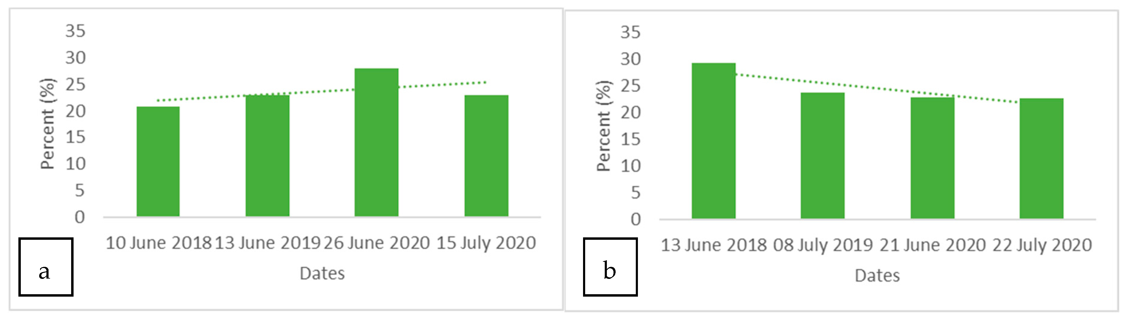
| Athens | 13 June 2018 | 94.80 | 0.9020 |
| 08 July 2019 | 91.80 | 0.8470 | |
| 21 June 2020 | 93.40 | 0.8783 | |
| 22 July 2020 | 92.87 | 0.8662 | |
| Bucharest | 10 June 2018 | 96.20 | 0.9267 |
| 13 June 2019 | 93.20 | 0.8739 | |
| 26 June 2020 | 95.00 | 0.9080 | |
| 15 July 2020 | 93.00 | 0.8700 |
| Date | Df between Groups | Df within Groups | F-Statistic/ p-Value | Class_Roads | Class_Center | Class_Built | |||
|---|---|---|---|---|---|---|---|---|---|
| NDVI | MSAVI2 | NDVI | MSAVI2 | NDVI | MSAVI2 | ||||
| Athens | |||||||||
| 13 June 2018 | 4 | 223966 | F | 357.03 | 348.71 | 4778.36 | 4580.19 | 4203.57 | 4347.13 |
| p | 0.00 | 0.00 | 0.00 | 0.00 | 0.00 | 0.00 | |||
| 8 July 2019 | 4 | 149844 | F | 428.16 | 413.18 | 2975.23 | 2984.12 | 2841.54 | 3006.98 |
| p | 0.00 | 0.00 | 0.00 | 0.00 | 0.00 | 0.00 | |||
| 21 June 2020 | 4 | 181283 | F | 385.94 | 369.83 | 5220.60 | 5085.26 | 4531.01 | 4743.90 |
| p | 0.00 | 0.00 | 0.00 | 0.00 | 0.00 | 0.00 | |||
| 22 July 2020 | 4 | 242108 | F | 180.10 | 203.38 | 3548.11 | 3484.79 | 3789.40 | 3897.32 |
| p | 0.00 | 0.00 | 0.00 | 0.00 | 0.00 | 0.00 | |||
| Bucharest | |||||||||
| 10 June 2018 | 4 | 91753 | F | 34.32 | 63.79 | 5.83 | 256.52 | 1.34 | 42.52 |
| p | 0.00 | 0.00 | 0.00 | 0.00 | 0.25 | 0.00 | |||
| 13 June 2019 | 4 | 92611 | F | 32.75 | 32.91 | 340.22 | 351.81 | 144.91 | 126.52 |
| p | 0.00 | 0.00 | 0.00 | 0.00 | 0.00 | 0.00 | |||
| 26 June 2020 | 4 | 107680 | F | 26.87 | 26.24 | 230.55 | 217.16 | 116.02 | 107.57 |
| p | 0.00 | 0.00 | 0.00 | 0.00 | 0.00 | 0.00 | |||
| 15 July 2020 | 4 | 100240 | F | 518.35 | 507.65 | 2274.74 | 2216.17 | 1206.33 | 1182.90 |
| p | 0.00 | 0.00 | 0.00 | 0.00 | 0.00 | 0.00 | |||
| City | Date | Rainfall (mm) | Rainy Days (No.) | Average Temperature (°C) |
|---|---|---|---|---|
| Athens | 13 June 2018 | 0 | 0 | 24.1 |
| 8 July 2019 | 0 | 0 | 27.1 | |
| 21 June 2020 | 0 | 0 | 21.5 | |
| 22 July 2020 | 0 | 0 | 26.3 | |
| Bucharest | 10 June 2018 | 31 | 9 | 21.2 |
| 13 June 2019 | 157 | 14 | 20.1 | |
| 26 June 2020 | 109 | 14 | 19.8 | |
| 15 July 2020 | 83 | 9 | 23.7 |
Publisher’s Note: MDPI stays neutral with regard to jurisdictional claims in published maps and institutional affiliations. |
© 2022 by the authors. Licensee MDPI, Basel, Switzerland. This article is an open access article distributed under the terms and conditions of the Creative Commons Attribution (CC BY) license (https://creativecommons.org/licenses/by/4.0/).
Share and Cite
Popa, A.M.; Onose, D.A.; Sandric, I.C.; Dosiadis, E.A.; Petropoulos, G.P.; Gavrilidis, A.A.; Faka, A. Using GEOBIA and Vegetation Indices to Assess Small Urban Green Areas in Two Climatic Regions. Remote Sens. 2022, 14, 4888. https://doi.org/10.3390/rs14194888
Popa AM, Onose DA, Sandric IC, Dosiadis EA, Petropoulos GP, Gavrilidis AA, Faka A. Using GEOBIA and Vegetation Indices to Assess Small Urban Green Areas in Two Climatic Regions. Remote Sensing. 2022; 14(19):4888. https://doi.org/10.3390/rs14194888
Chicago/Turabian StylePopa, Ana Maria, Diana Andreea Onose, Ionut Cosmin Sandric, Evangelos A. Dosiadis, George P. Petropoulos, Athanasios Alexandru Gavrilidis, and Antigoni Faka. 2022. "Using GEOBIA and Vegetation Indices to Assess Small Urban Green Areas in Two Climatic Regions" Remote Sensing 14, no. 19: 4888. https://doi.org/10.3390/rs14194888
APA StylePopa, A. M., Onose, D. A., Sandric, I. C., Dosiadis, E. A., Petropoulos, G. P., Gavrilidis, A. A., & Faka, A. (2022). Using GEOBIA and Vegetation Indices to Assess Small Urban Green Areas in Two Climatic Regions. Remote Sensing, 14(19), 4888. https://doi.org/10.3390/rs14194888