Unsupervised Domain Adaptation for Remote Sensing Semantic Segmentation with Transformer

Abstract

With the development of deep learning, the performance of image semantic segmentation in remote sensing has been constantly improved. However, the performance usually degrades while testing on different datasets because of the domain gap. To achieve feasible performance, extensive pixel-wise annotations are acquired in a new environment, which is time-consuming and labor-intensive. Therefore, unsupervised domain adaptation (UDA) has been proposed to alleviate the effort of labeling. However, most previous approaches are based on outdated network architectures that hinder the improvement of performance in UDA. Since the effects of recent architectures for UDA have been barely studied, we reveal the potential of Transformer in UDA for remote sensing with a self-training framework. Additionally, two training strategies have been proposed to enhance the performance of UDA: (1) Gradual Class Weights (GCW) to stabilize the model on the source domain by addressing the class-imbalance problem; (2) Local Dynamic Quality (LDQ) to improve the quality of the pseudo-labels via distinguishing the discrete and clustered pseudo-labels on the target domain. Overall, our proposed method improves the state-of-the-art performance by 8.23% mIoU on Potsdam→Vaihingen and 9.2% mIoU on Vaihingen→Potsdam and facilitates learning even for difficult classes such as clutter/background.

1. Introduction

Remote sensing (RS) image-semantic segmentation is aimed at analyzing the pixel-level content of RS images and classifying each pixel in RS images with a predefined ground truth label. It has received increasing attention and research interest due to its application in city planning, flood control, and environmental monitoring.

In the past few years, many semantic segmentation algorithms based on deep neural networks (DNNs) have been proposed and achieved overwhelming performance, such as fully convolutional networks [1,2,3], Encoder-Decoder based models [4], and Transformers [5,6,7,8]. However, these methods require a large amount of annotated data to work properly with specific datasets and have degraded performance due to the discrepancy between feature distributions in different datasets and named domain gap (or domain shift). Datasets with different feature distributions are considered as different domains. The domain gap mainly occurs due to the diversity of data acquisition conditions, such as color, lighting, and camera settings. Therefore, in practical applications, these supervised methods are limited to specific scenes and still need laborious annotations to perform well in different datasets.

Domain adaptation (DA), a subcategory of transfer learning, has been recently proposed to address the domain gap. It enables a model to learn and transfer the domain-invariant knowledge between different domains. DA methods can be supervised, semi-supervised or unsupervised based on whether it has access to the labels of the target domain. In particular, unsupervised domain adaptation (UDA) is aimed at transferring the model from a labeled source domain to an unlabeled target domain. Currently, existing UDA works can be divided into generative-based methods, adversarial-learning methods, and self-training (ST) methods [9].

Specifically, generative-based works use image translation or style transferring to make the images from different domains visually similar. Then, semantic segmentation models can be trained with the translated images and the original labels. Yang et al. [10] used the Fast Fourier Transform (FFT) to replace the low-level frequencies of the target images with that of the source images before reconstituting the image via the inverse FFT. Ma et al. [11] adopted gamma correction and histogram mapping on source images to perform distribution alignment in a Lab color space. In remote sensing, graph matching [12] and histogram matching [13] were applied to perform image-to-image translation. To obtain more accurate and appropriate translation results, generative adversarial networks (GANs) [14,15,16,17] have been widely used in previous UDA methods [18,19,20,21,22,23] for RS semantic segmentation. The potential issue of generative-based methods is that the performance of semantic segmentation models heavily rely on the quality of translated images, as pixel-level flaws could significantly influence the accuracy.

Adversarial-learning methods introduce a discriminator network to help segmentation networks minimize the discrepancy between source and target feature distributions. The segmentation network predicts the segmentation results for the source and target images. The discriminator takes the feature maps from the segmentation network and tries to predict the domain of the input. To fool the discriminator, the segmentation network finally outputs feature maps with similar distribution for images from the source and target domains. Tsai et al. [19] established that source and target domains share strong similarities in semantic layout. They constructed a multi-level adversarial network to exploit structural consistency in the output space across domains. Vu et al. [24] used a discriminator to make the target’s entropy distribution similar to the source. Cai et al. [21] proposed a bidirectional adversarial-learning framework to maintain bidirectional semantic consistency. However, the discriminator networks are highly sensitive to hyper-parameters and are difficult to train to learn similar feature distributions in different domains.

Unlike the first two UDA methods, self-training (ST) methods do not rely on any auxiliary networks. ST strategies can transfer knowledge across domains with segmentation networks only, which is far more elegant. ST methods follow the “easy-to-hard” scheme where the highly confident predictions inferred from unlabeled target data are treated as pseudo-labels and the labeled source data and pseudo-labeled target data are used jointly to get a better performance in the target domain. Zou et al. [25] proposed one of the first iterative ST techniques in semantic segmentation by treating pseudo-labels as discrete latent variables, which are computed through the minimization of a unified training objective. Vu et al. [24] introduced direct entropy minimization to self-training as a way to encourage the model to produce high-confident predictions instead of using a threshold to indicate high-confident ones. Yan et al. [26] combined the self-learning method with the adversarial-learning method on RS images by a cross-mean teacher framework exploiting the pseudo-labels near the edge. To alleviate the issue of faulty UDA pseudo-labels in semantic segmentation, each pseudo-label is weighted by the proportion of pixels with confidence above a certain threshold [27,28], named the quality of pseudo-labels.

In addition, most previous UDA methods evaluate their performance with classical architectures such as DeepLabV2 [29] and DeepLabV3+ [4] which have been outperformed by the modern vision transformer [5,6,7] and limit the overall performance of UDA methods. In recent studies, Xu et al. [7] first introduced the transformer into the supervised semantic segmentation of RS images. Hoyer et al. [30] were also the first to systematically study the influence of recent transformer architectures on UDA semantic segmentation.

Meanwhile, UDA is concerned with transferring knowledge from a labeled domain to an unlabeled domain, which is domain-relevant. From the perspective of domain-irrelevant methods, we can focus on improving the generalization of models by increasing the size of training data and addressing the class-imbalance problem.

Data augmentation, a technique of generating perturbed images, has been found to improve the generalization ability of models in various tasks. For instance, Zhang et al. [31] enhanced the dataset by linear combinations of data and corresponding labels. Yun et al. [32] composited new images by cutting a rectangular region from one image and pasting it on another, a technique recently adopted by Gao et al. [22] for semantic segmentation of RS images. Chen et al. [33] used a variety of spatial/geometric and appearance transformations to learn good representations and gain great accuracy by a simple classification model in a self-supervised learning method. In semi-supervised learning, Olsson et al. [27] mixed unlabeled data to generate augmented images and labels named ClassMix. The mask’s shape for mixing is determined by category and is not necessarily rectangular. To be specific, a mask may contain all the pixels of a class. However, in the strategy of ClassMix, half of the classes are selected to generate the mask [27]. Then, it was developed by Tranheden et al. [28] in the image-semantic segmentation UDA task, where the masked slices of images and labels are generated in the source domain and are pasted to the target domain, thus making the target images contain slices of the source images.

The imbalanced category proportions compromise the performance of most standard learning algorithms, which expect balanced class distributions. When presented with complex imbalanced datasets such as RS datasets, these algorithms might fail to properly represent the distributive characteristics of the data, thus providing unfavorable accuracy across the classes of the data. To address the class-imbalance problem, basic strategies can be divided into two categories, i.e., preprocessing and cost-sensitive learning [34]. However, most of them have either high computational complexities or many hyper-parameters to tuning. In deep learning, Zou et al. addressed the class-imbalance problem by setting different class weights based on the inverse of their corresponding proportions in the dataset [25]. In UDA, Yan et al. [35] introduced class-specific auxiliary weights for exploiting the class prior probability on source and target domains. Recently, Hoyer et al. [30] sampled source data with rare classes more frequently in order to learn them better and earlier. On the other hand, some data with common classes may be rarely sampled or not sampled at all, which might result in degraded performance.

However, three challenges still exist in UDA for RS image-semantic segmentation: (i) The potential of a vision Transformer for UDA semantic segmentation of RS images has not been discussed. (ii) In ST methods [27,28], the correct and incorrect pseudo-label in an image gets the same weight depending on the ratio of high-confident pixels. (iii) Due to the randomness of sampling, the changes in category proportions during the training process have not been considered in [30,35] for addressing the class-imbalance problem in UDA semantic segmentation.

In this paper, we apply Transformer [30] and cross-domain mixed sampling [28] to a self-training UDA framework for RS image-semantic segmentation. Then, two strategies are proposed to boost the performance of the framework. First, we introduce a strategy of Gradual Class Weights to dynamically adjust class weights in the source domain for addressing the class-imbalance problem. Secondly, a novel way to calculate the quality of pseudo-labels is proposed to guide the adaptation to the target domain. The implementation code is available at https://github.com/Levantespot/UDA_for_RS, accessed on 21 August 2022. The three main contributions of our work can be summarized as follows:

1.

We demonstrate the remarkable performance of Transformer in self-training UDA of RS images compared to the previous methods using DeepLabV3+ [4];

2.

Two strategies, Gradual Class Weights, and Local Dynamic Quality are proposed to improve the performance of the self-training UDA framework. Both of them are easy to implement and embed in any existing semantic segmentation model;

3.

We outperformed state-of-the-art UDA methods of RS images on the Potsdam and Vaihingen datasets, which indicates that our method can improve the performance of cross-domain semantic segmentation and minimize the domain gap effectively.

2. Methods

In this section, we provide an overview of our self-training framework, where the pseudo-labels $p_T$ are generated by teacher model $h_{\varphi }$ from the target images $x_T$ to guide the student network $g_{\theta }$ to better transfer knowledge from the source to the target domain. In addition, we will briefly compare the difference between the network structure of the convolutional neural network (CNN) and the vision Transformer. Then, the class imbalance issue is alleviated by Gradual Class Weights (GCW), where the weights of classes are updated based on the current source image $x_S$. Finally, we illustrate the implementations of the Local Dynamic Quality (LDQ), where the quality of pseudo-labels $p_T$ is estimated based on the states of their neighbors. The overall self-training UDA framework is shown in Figure 1.

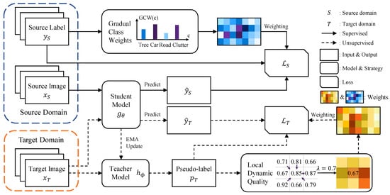
Figure 1. Overview of our self-training framework with Gradual Class Weights and Local Dynamic Quality. Source images $x_S$ and source labels $y_S$ are trained together in a supervised way with GCW. Pseudo-labels $p_T$ are generated by teacher model $h_{\varphi }$ in place of the target labels $y_T$. Target images $x_T$ and pseudo-labels $p_T$ are trained together with LDQ. The darker the color is in GCW and LDQ, the larger the weight of the corresponding class and pseudo-label is.

2.1. Self-Training (ST) for UDA

In UDA for RS, we define two sets of images collected from different satellites or locations as different domains. To simplify the problem, images in the source and target domains have the same resolution of $H\times W$ with 3 channels and the same set of semantic classes in both domains. One having both images $x_S$ and corresponding labels $y_S$ is the source domain ${\mathcal{D}}_S=\left\{(x_S,y_S)\right|x_S\in {\mathbb{R}}^{H\times W\times 3},y_S\in {\mathbb{R}}^{H\times W\times C}\}$, where C is the number of categories while the other with only images $x_T$ available is known as the target domain ${\mathcal{D}}_T=\left\{x_T\right|x_T\in {\mathbb{R}}^{H\times W\times 3}\}$. The subscripts S and T denote the source and target domains, respectively. Note that the target labels $y_T$ are only accessible at the testing stage. The label at spatial location $(h,w)$ in $y_S$ is a one-hot vector with a length of C, denoted as $y_S^{(h,w)}$, $h\in [1,\dots ,H],w\in [1,\dots ,W]$. The objective of UDA methods is to train a model using source images $x_S$ and source labels $y_s$ to achieve a good performance on target images $x_T$ without having access to the target labels $y_T$. In the self-training UDA framework, a student model $g_{\theta }$ is first trained on the source domain ${\mathcal{D}}_S$ in a supervised way, where $\theta$ denotes its parameters. The objective function with cross-entropy loss is formulated as shown in Equation (1):

$${\mathcal{L}}_S(x_S,y_S)=-\sum _{c=1}^C\sum _{h=1}^H\sum _{w=1}^W\mathrm{GCW}(n,c)·{\left(y_S^{(h,w)}\right)}_c·log{\left(g_{\theta }\left(x_S^{(h,w)}\right)\right)}_c$$

(1)

where $x_S$,$y_S$ are the n-th source image and the corresponding label, ${(·)}_c$ denotes the c-th scalar of a vector, $g_{\theta }\left(x_S^{(h,w)}\right)\in {\mathbb{R}}^C$ denotes the normalized probabilities predicted by $g_{\theta }$ of each class at location $(h,w)$ in image $x_S$, and $\mathrm{GCW}(n,c)$ is the weight as a function of class c and index n of the image and will be discussed in Section 2.3.

To address the domain gap, ST approaches use pseudo-labels $p_T$ to transfer the knowledge from the source to the target domain. In the basic version of ST methods, the student model generates the pseudo-labels $p_T$. To reduce abrupt changes in the model parameters due to the large gap between the source and target domains, the exponentially moving average (EMA) and teacher model $h_{\varphi }$ are introduced to make the generation of pseudo-labels more reliable. In EMA, the teacher model $h_{\varphi }$ is updated based on the student model $g_{\theta }$, formulated as shown in Equation (2):

$${\varphi }_{t+1}\leftarrow \alpha {\varphi }_t+(1-\alpha ){\theta }_t$$

(2)

where $\theta$ and $\varphi$ are the parameters of student model $g_{\theta }$ and teacher model $h_{\varphi }$, respectively, t denotes the training step, and hyper-parameter $\alpha \in [0,1]$ indicates how important the current state of weights ${\varphi }_t$ is. The generation of pseudo-labels $p_T$ is formulated as shown in Equation (3):

$${(p_T^{(h,w)})}_c=\left\{\begin{array}{cc}1,\hfill & \mathrm{if}c=\underset{c^{\prime }}{argmax}{\left(h_{\varphi }(x_T^{(h,w)})\right)}_{c^{\prime }}\hfill \\ 0,\hfill & \mathrm{otherwise}\hfill \end{array}\right.$$

(3)

where $p_T^{(h,w)}$ denotes the one-hot pseudo-label at location $(h,w)$ in the pseudo-labels $p_T$, and $h_{\varphi }(x_T^{(h,w)})\in {\mathbb{R}}^C$ denotes the normalized probabilities of each class in image $x_T$ at location $(h,w)$. Note that no gradient will be backpropagated into the teacher model $h_{\varphi }$ through this procedure. Since there is no guarantee that these generated pseudo-labels are corrected, we use LDQ to quantify the reliability and quality of each pseudo-label at location $(h,w)$. They are denoted as $LDQ(h,w)$ and will be discussed later in Section 2.4. The pseudo-labels $p_T$ and their quality are jointly used to train on the target domain as shown in Equation (4):

$${\mathcal{L}}_T(x_T,p_T)=-\sum _{h=1}^H\sum _{w=1}^W\mathrm{LDQ}(h,w)·p_T^{(h,w)}·log{g}_{\theta }(x_T^{(h,w)})$$

(4)

Note that the models $g_{\theta }$ and $h_{\varphi }$ have the same network architecture. The pseudo-labels $p_T$ are generated online, i.e., the teacher model $h_{\varphi }$ generates pseudo-labels $p_T$ for every image at each iteration.

2.2. Transformer for Semantic Segmentation

We will briefly review what makes CNNs successful and then compare them to the key components of vision Transformers. Generally, CNNs leverage the basic information such as texture and color that make up the visual elements through a large number of convolutional filters. For example, convolutional filters capture the key points, lines, and curves in shallow layers, while filters in deeper layers extract more abstract details and focus on discriminative structures [36,37]. Since CNNs are locally sensitive, different receptive fields (RF) of the input image are perceived in different layers, as shown in Figure 2. From the perspective of information flow, the receptive field determines the area where the model can learn the information of the input image. Furthermore, CNNs capture local structures of an image in the early stages and extract a larger range of global features in the deeper layers.

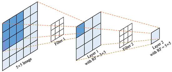
Figure 2. The receptive fields of CNNs in different layers. As the convolution proceeds, the range of receptive fields gradually increases. Layer 1 gets an RF of 3 × 3 (blue area in the image), while 5 × 5 for layer 2 (light blue area in the image). Note that the two filters are both fixed at testing.

However, the learned convolutional filters are fixed at testing, which hinders the generalization of CNNs. To make the model more adaptive and general, vision Transformers [5,6,7,8] bring the self-attention mechanism from natural language processing to computer vision. The self-attention mechanism is illustrated in Figure 3. The fixed convolutional filters are replaced with weights that can be computed dynamically based on the similarity or affinity between every pair of patches, thus enabling capturing “long-term” information and dependencies between sequence elements. Therefore, vision Transformers have a larger receptive field to extract finer features at the encoding stage.

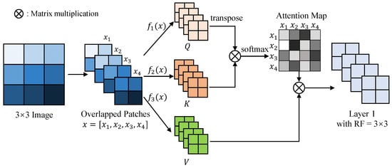
Figure 3. A simplified illustration of the self-attention mechanism in vision Transformer. The self-attention mechanism takes the overlapped patches of an image as input. These patches are encoded in three ways, i.e., $f_1,f_2,f_3$, to get three matrices Q, K, V, short for Query, Key, and Value, respectively. The softmax result of the matrix product of Q and K is called the attention map, which represents the similarity or weights between each pair of patches. The darker the color in the attention map, the stronger the relationship between the two patches. The attention map is multiplied with the matrix V to get the feature layer 1, which is the output of the self-attention module. Unlike the convolution, self-attention module has a receptive field of the entire input.

2.3. Gradual Class Weights (GCW)

Class imbalance is a common and plaguing situation where the distribution of data is skewed since some classes appear much more frequently than others. For example, the common class roads occur more frequently than the rare class cars, resulting in less information about the cars and poor model generalization. To efficiently alleviate this issue, Zou et al. [25] assigned a weight to each class, inversely proportional to the frequency in the whole training dataset. As a result, the rare classes receive more attention than the common classes. The frequency $f_c$ of class c is defined in Equation (5):

$$f_c=\frac{1}{H\times W}\sum _{h=1}^H\sum _{w=1}^W{(y_S^{(h,w)})}_c$$

(5)

where $y_S^{(h,w)}$ denotes the one-hot source label at location $(h,w)$, and ${(·)}_c$ denotes the c-th scalar of a vector. However, due to the randomness in sampling, the distribution of the class will be different from that calculated on the whole dataset in advance. To address the mismatched distribution, the weights will be updated iteratively for each image. In addition, inspired by gradual warmup [38], where small learning rates are used to reduce volatility in the early stages of training, it is assumed that class weights also need the warmup to keep the model more stable and robust in the early training stages. Notably, instead of directly initializing the class weights to the distributions estimated from the first sample, they are initialized to 1 and then are updated iteratively by an exponentially weighted average. The pseudo-code of the proposed GCW is presented in Algorithm 1, where ${\mathcal{Y}}_S$ denotes all the source labels with a size of $N_s$, $f_c$ denotes the frequency of class c in the source domain, $\mathrm{W}(n,c)$ represents the original class weights only based on $f_c$, and T denotes the temperature parameter [30]. A higher T leads to a more uniform distribution while a lower one makes the model pay more attention to the rare classes.

Algorithm 1 Gradual Class Weights

Input: Source Labels ${\mathcal{Y}}_S\in {\mathbb{R}}^{N_S\times H\times W\times C}$, mixing parameter $\beta \in (0,1)$, and temperature T. Output: Gradual class weights $\mathrm{GCW}(n,c)$ for each class c of n-th image. 1: $\forall c\in [1,\cdots ,C],\mathrm{GCW}(0,c)\leftarrow 1$           ▹ Initialization via equal weights. 2: forn = 1 to $N_s$ do                   ▹ Calculate GCW for each image. 3:     $y_S\leftarrow {\mathcal{Y}}_S\left(n\right)$                       ▹ Get n-th label from ${\mathcal{Y}}_S$. 4:     for c = 1 to C do                            ▹ For each class 5:         $W(n,c)=\frac{C·exp[(1-f_c)/T]}{{\sum }_{c^{\prime }=1}^{C}exp[(1-f_{c^{\prime }})/T]}$           ▹ Calculate the naive class weights. 6:         $\mathrm{GCW}(n,c)=\beta ·\mathrm{GCW}(n-1,c)+(1-\beta )·\mathrm{W}(n,c)$      ▹ Calculate the GCW. 7:     end for 8: end for

2.4. Local Dynamic Quality (LDQ) of Pseudo-Labels

In some previous ST works [25,26], only pseudo-labels with probabilities greater than a fixed threshold $\lambda$ are used for training, and they are known as high-quality pseudo-labels. Equation (6) depicts the procedure of determining the quality of the pseudo-label at location $(h,w)$.

$$q(h,w)=\left\{\begin{array}{cc}1,\hfill & \mathrm{if}max\left(h_{\varphi }(x_T^{(h,w)})\right)\ge \lambda \hfill \\ 0,\hfill & \mathrm{otherwise}\hfill \end{array}\right.$$

(6)

where 1 and 0 indicate high quality and low quality, respectively, $h_{\varphi }$ denotes the teacher model used to generate pseudo-labels as it is more stable than the student model $g_{\theta }$. The threshold $\lambda$ is typically determined via grid search, where a manually specified subset of the thresholds is searched exhaustively, the best value will then be chosen as the pseudo-label threshold $\lambda$. Once the threshold is determined, it will not be changed during the training stage. Intuitively, a higher threshold leads to more accurate, high-quality pseudo-labels but may also result in fewer samples available for training in the early training stage, because the model should have lower confidence during the early training stages than after many iterations.

To alleviate the influence of faulty UDA pseudo-labels in semantic segmentation, the image-wise ratio of high-quality pseudo-labels in an image is estimated to weigh the sample [27,28]. Therefore, we proposed a pixel-wise quality of pseudo-labels named local dynamic quality (LDQ), where each pseudo-label is assigned a different weight based on the pixels around it. The main idea underlying our method is intuitive: discrete pseudo-labels are more likely to be misclassified and should have relatively lower quality. On the contrary, the clustered ones deserve higher quality. In particular, the quality of a pseudo-label is calculated based on the ratio of high-quality surrounding pseudo-labels, which can be efficiently calculated through convolution. The formula for LDQ is demonstrated in Equation (7):

$$LDQ(h,w)=\frac{1}{{(2K+1)}^2}\sum _{i=-K}^K\sum _{j=-K}^{K}q(h+i,w+j)$$

(7)

where $LDQ(h,w)$ denotes the quality of a pseudo-label at location $(h,w)$, $K\in \mathbb{N}$ denotes the depth of neighbors, and $2K+1$ is known as the size of the convolution kernel. In contrast to [25,26], all pseudo-labels, correct or incorrect, are used for training as the pixels-wise quality weights the influence of each pseudo-label.

3. Results

In this section, we introduce the source and target datasets, describe the experimental details, and finally illustrate the obtained results.

3.1. Dataset Description

The Potsdam (POT) dataset [39] contains 38 patches of a typical historic city with large building blocks, narrow streets, and dense settlement structures with a resolution of 6000 × 6000 pixels over Potsdam City, and the ground sampling distance is 5 cm. In total, 24 and 14 patches are used for training and testing, respectively.

The Vaihingen (VAI) dataset [40] contains 33 patches of a relatively small village with many detached buildings and few multi-story buildings with a resolution ranging from 1996 × 1995 to 3816 × 2550 pixels, and the ground sampling distance is 9 cm. In total, 16 and 17 patches are used for training and testing, respectively.

Both datasets have the same six categories: impervious surfaces, buildings, low vegetation, trees, cars, and clutter/background. The clutter/background class consists of water bodies and other objects which are of no interest in semantic object classification in urban scenes. Note that Potsdam has two band modes; RGB (red, green, and blue) and IRRG (near-infrared, red, and green), while Vaihingen has only IRRG mode. We use Potsdam in RGB mode and Vaihingen in IRRG mode. In IRRG mode, things may look different from natural images, e.g., trees and low vegetation are red. Since Potsdam is a city and Vaihingen is a village, there are more cars and apartments in the POT dataset, while there are more houses and farmland in the VAI dataset.

Since the two datasets are the same in task objective and label space but different in feature distribution and band mode, they are suitable for evaluating the performance of UDA methods. In this paper, we used two different settings of domain adaptation. The first one is transferring from the Potsdam dataset to the Vaihingen dataset, presented as POT→VAI, and the other is the opposite, denoted as VAI→POT. Note that the only difference between the source and target domains is that no labels are accessible in the target domain during training. Meanwhile, to make images and labels fit into the GPU memory properly, all images are cropped into 512 × 512 pixels’ patches with overlaps of 256 pixels. In this setting, 344 training data and 398 testing data are generated from VAI, while 3456 and 2016 are for POT.

3.2. Implementation Details

Preprocessing: Our implementation is based on the PyTorch [41] and MMSegmentation [42]. We use the preprocessing pipeline provided by the MMSegmentation [42], where resizing, cropping, flipping, normalization, and padding are randomly applied to the data. The pixels between the boundaries are ignored during training. In accordance with [28,30], we mix the target data with the source data in the same way and use the same data augmentation parameters of colorjitter, where the brightness, contrast, saturation, and hue of images are randomly changed.

Network Architecture: Since both local and global features are important in semantic segmentation, feature fusion [4] is usually required in CNNs to obtain high-precision segmentation results. Hoyer et al. [30] designed a Transformer with context-aware multilevel feature fusion, named DAFormer, to exploit both coarse-grained and fine-grained features. Since they achieved the best results in UDA semantic segmentation, we adopt DAFormer [30] as the network architecture for both student model $g_{\theta }$ and teacher model $h_{\varphi }$. DAFormer [30] used the MiT-B5 encoder [6] pre-trained on ImageNet [43] to produce a feature pyramid with channels = [64, 128, 320, 512]. Then, its decoder embeds each feature to 256 channels with the same size of $\frac{H}{4}\times \frac{W}{4}$, followed by the depth-wise dilated separable convolutions [44] with the dilation rates of 1, 6, 12, and 18.

Training: Student model $g_{\theta }$ is trained with the AdamW [45] optimizer using betas = (0.9, 0.999), a learning rate of $1\times {10}^{-4}$ for the encoder and $1\times {10}^{-3}$ for the decoder, a weight decay of 0.01, linear learning rate warmup with $t_{warm}=1500$, and linear decay of 0.01 afterwards. The $\alpha$ used to update the teacher model $h_{\varphi }$ is set to $0.99$. Then, two networks are trained for 4000 iterations with a batch size of 8 consisting of 4 source and 4 target data. For GCW, the temperature T is set to 0.1 to pay more attention to the pixels of the rare class, and the mixing parameter $\beta$ is set to 0.9 to smoothly update the class distribution. In LDQ, we set the threshold of pseudo-labels $\lambda$ to $0.7$.

3.3. Quantitative Results

In accordance with the previous UDA methods of RS semantic segmentation, F1-score and Intersection over Union (IoU) have been used to evaluate the methods. The metrics are formulated as shown in Equations (8) and (9):

$$\mathrm{IoU}=\frac{TP}{TP+FP+FN}$$

(8)

$$\mathrm{F}1\text{-}\mathrm{score}=\frac{2\times TP}{2TP+FP+FN}$$

(9)

where $TP$, $FP$, and $FN$ denote the number of true positive pixels, false positive pixels, and false negative pixels, respectively. IoU is also known as the Jaccard index, and the F1-score is known as the Dice coefficient.

Since there are six different classes in VAI and POT datasets, F1-score and IoU are first calculated for every class followed by the mean IoU (mIoU) and mean F1-score (mF1) calculated by averaging the results of all the classes. The results of our method are shown in four experiments and are reported in Table 1 and Table 2. We build our baseline (B/L) with a self-training framework (discussed in Section 2.1), DAFormer [30] network, the mixing strategy in [28], and learning rate warmup [38]. Then, GCW and LDQ are first added separately to the baseline and finally combined at the same time. To make our results more reliable, all results are obtained by averaging over three runs with the same parameters and architecture. Compared to the baseline on POT→VAI, GCW improves the performance by 9.97% of mIoU and 8.47% of mF1. It especially improves the performance of the roads, trees, and vegetation, while LDQ greatly increases the results of the clutter. As the two results of GCW and LDQ are complementary in many classes, our method generates more robust results when using both GCW and LDQ. On VAI→POT, the performance of LDQ is more desirable than GCW in the clutter, car, and tree classes, while it degraded in the vegetation class. In addition, the final experiment conducted with GCW and LDQ achieved close to optimum results. However, all the experiments generated inferior results close to zero in the clutter class on VAI→POT.

Table 1. Quantitative results (%) on POT→VAI.

Method	Clutter		Road		Car		Tree		Vegetation		Building		Overall
	IoU	F1	IoU	F1	IoU	F1	IoU	F1	IoU	F1	IoU	F1	mIoU	mF1
CycleGAN [16]	2.03	3.14	48.48	64.99	25.99	40.57	41.97	58.87	23.33	37.50	64.53	78.26	34.39	47.22
AdaptSegNet [19]	6.26	9.55	55.91	71.44	34.09	50.34	47.56	64.17	23.18	37.22	65.97	79.36	38.83	52.01
MUCSS [20]	3.94	13.88	46.19	61.33	40.31	57.88	55.82	70.66	27.85	42.17	65.44	83.00	39.93	54.82
RDG-OSA [23]	9.84	14.55	62.59	76.81	54.22	70.00	56.31	71.92	37.86	54.55	79.33	88.41	50.02	62.71
CSC-Aug [22]	8.12	11.23	68.91	81.48	57.41	72.76	65.47	79.04	48.33	64.78	81.78	89.94	55.00	66.54
Baseline	25.19	40.19	66.81	80.10	43.22	60.32	52.23	67.51	43.08	60.08	88.72	90.54	53.21	67.04
w. GCW	30.43	46.48	75.28	85.87	47.47	64.32	73.98	85.05	62.36	76.80	89.61	94.52	63.18	75.51
w. LDQ	37.90	54.79	67.12	80.30	40.31	57.39	58.68	72.55	45.15	61.85	89.78	94.62	56.49	70.25
w. GCW & LDQ	41.63	53.19	75.22	85.84	41.63	58.75	74.53	85.40	61.44	76.08	90.32	94.91	63.23	75.70

Clutter, Road, and Vegetation indicate Clutter/Background, Impervious Surface, and Low Vegetation, respectively. The same applies to Table 2.

Table 2. Quantitative results (%) on VAI→POT.

Method	Clutter		Road		Car		Tree		Vegetation		Building		Overall
	IoU	F1	IoU	F1	IoU	F1	IoU	F1	IoU	F1	IoU	F1	mIoU	mF1
CycleGAN [16]	10.77	16.66	50.91	66.91	43.72	59.82	32.23	48.08	24.19	37.93	62.73	76.32	37.43	50.95
AdaptSegNet [19]	2.24	3.67	46.71	63.07	45.44	61.92	21.23	34.26	29.84	44.86	50.49	66.56	32.66	45.72
MUCSS [20]	13.56	23.84	45.96	62.97	39.71	56.84	25.80	40.97	41.73	58.87	59.01	74.22	37.63	52.95
RDG-OSA [23]	3.02	3.82	59.76	74.35	60.62	74.83	43.50	59.92	40.65	56.73	73.30	84.13	46.81	58.96
Baseline	0.25	0.50	59.60	73.86	26.13	32.14	48.76	65.51	41.98	59.10	71.13	82.69	41.31	52.30
w. GCW	0.65	1.29	64.81	78.53	48.05	56.39	34.05	50.60	37.82	54.60	73.13	84.40	43.08	54.30
w. LDQ	0.85	1.65	57.73	73.05	68.81	81.52	41.52	58.64	6.91	12.52	73.92	84.97	41.62	52.06
w. GCW & LDQ	0.53	1.04	71.15	82.94	65.53	79.18	56.63	72.23	59.53	74.60	82.68	74.04	56.01	66.73

The results of VAI→POT are not provided by CSC-Aug [22].

3.4. Visualization Results

Figure 4 and Figure 5 depict the predicted results for baseline, baseline with GCW, baseline with LDQ, and baseline with GCW and LDQ on POT→VAI and VAI→POT, respectively. Note that the thick black lines in panels (b) are the boundaries ignored during training.

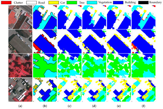
Figure 4. Predictions of the validation images from VAI on POT→VAI. (a) Target images. (b) Ground truth. (c) Baseline. (d) Baseline with GCW. (e) Baseline with LDQ. (f) Baseline with GCW and LDQ.

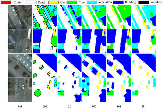
Figure 5. Predictions of the validation images from POT on VAI→POT. (a) Target images. (b) Ground truth. (c) Baseline. (d) Baseline with GCW. (e) Baseline with LDQ. (f) Baseline with GCW and LDQ.

3.5. Comparisons with Other Methods

We compare our results with five methods of remote sensing domain adaptation: CycleGAN [16] is a generative network transferring images from a source domain to a target domain, AdaptSegNet [19] is a multi-level adversarial discriminator network exploiting structural consistency, MUCSS [20] combines DualGAN [15] network with ST strategies, CSC-Aug [22] combines style translation with the consistency principle, and RDG-OSA [23] proposed the resize-residual DualGAN [15] with an output space adaptation method. These previous UDA works use either DeepLabv2 [29] or DeepLabv3+ [4] as the semantic segmentation framework. Note that the results of all methods are using the same datasets POT and VAI. In addition, we take the average results of all methods to ensure fairness. A comprehensive comparison with these works is shown in Table 1 and Table 2 for POT→VAI and VAI→POT, respectively.

Our baseline is surprisingly competitive and even better compared to other state-of-the-art techniques, which demonstrates that the Transformer generalizes better to the new domain than the previous CNNs. Compared to CSC-Aug [22], our method increases the mIoU and mF1 by 8.23% and 9.16% on POT→VAI, respectively. While compared to RDG-OSA [23], it increases by 9.2% and 7.77%, respectively, on VAI→POT. Generally, our proposed method almost outperforms all the previous works both in IoU and F1-score, except for the car class on POT→VAI and the clutter class on VAI→POT.

4. Discussion

In this section, we first explore strategies and hyper-parameters in detail. Since our experiments show that the results on POT→VAI are more stable and reliable than that on VAI→POT, we focus on the consequences of the strategies mainly via experiments on POT→VAI. Then, we discuss the limitations of the proposed method, the possible reasons for unstable results on VAI→POT, and possible further improvements.

4.1. GCW

In supervised learning, it is often beneficial to change the loss weights of each class to obtain better performance because most datasets are class-imbalanced. However, it is more complicated in domain adaptation problems where the same class may have different or conflicting feature and texture distributions in the source and target domains. Therefore, we investigate the influence of the class weights on UDA performance via three experiments, where the first one equally sets the weights of all classes to 1, the second experiment applies GCW to dynamically change the class weights, and the last experiment initializes the class weights to the final result of GCW as the final weights are approximately equal to the mean of those calculated from the entire dataset. All experiments are performed based on the baseline. Table 3 shows that the GCW can improve the performance of each class compared to the first approach, while the prior invariant weights in the third method severely degrade the results.

Table 3. The IoU (%) of each class with different class weights on POT→VAI.

Class Weight	Clutter	Road	Car	Tree	Vegetation	Building	Overall
Equal weights	25.19	66.81	43.22	52.23	43.08	88.72	53.21
GCW	30.43	75.28	47.47	73.98	62.36	89.61	63.18
Fixed prior weights	0.54	32.78	3.89	0.16	0	75.41	18.8

Figure 6 illustrates the change process of the class weights calculated by GCW, where the class weights of road, building, and vegetation are close to 0.5 while that of the car and clutter class are higher than 1.5, which indicates that the latter two appear much less frequently than the first three. Remarkably, most of the class weights at 800 iterations of training are close to themselves in the final rounds, which means that GCW and the third method are almost identical after 800 rounds. However, the model gets no extra performance by directly initializing the class weights to the final values but the degraded behaviors, as demonstrated in Figure 7. Therefore, we conclude that the proposed GCW that gradually adjusts the class weights serves by avoiding a sudden change of the class weights and allowing healthy convergence at the start of training, which is similar to a gradual warmup [38]. It reveals the significance of model stability in the UDA: the model could get unsatisfied results even if it performs well in early iterations because of the disagreement of feature distribution between the source and target domains. On the other hand, while the result curves of the GCW and equal weights have similar trends in Figure 7, the former has a higher IoU and more compact confidence interval almost for all the categories and iterations, indicating better performance and stability, respectively. To sum up, the model of UDA can still benefit from the well-focused class weights tenderly.

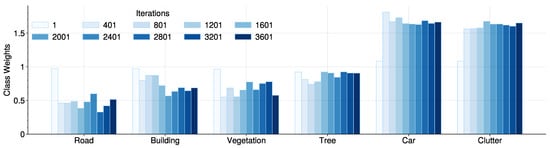
Figure 6. The weights of each category as calculated by GCW during the training on POT→VAI.

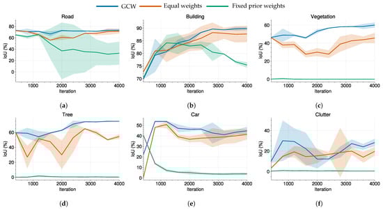
Figure 7. IoU of each category during the training on POT→VAI. The shaded areas correspond to the 95% confidence intervals. (a) Road. (b) Building. (c) Vegetation. (d) Tree. (e) Car. (f) Clutter.

4.2. LDQ

To begin, we compare our pixel-wise Local Dynamic Quality with the equal quality and image-wise quality [28,30] in Table 4. It should be noted that the results for the hyper-parameters discussed later are for LDQ applied alone. When LDQ and GCW are used together, we find that the best experimental results are obtained with different hyper-parameters. To be consistent with experiments in Table 1, we used the same $\lambda =0.7$ or $K=3$ in the following experiments. In equal quality, all generated pseudo-labels are considered correct. In addition, image-wise quality assigns the proportion of pseudo-labels exceeding a threshold $\lambda$ of the maximum softmax probability to all these pseudo-labels. In Table 4, our strategy of pixel-wise quality has the best overall performance among these methods. The performance improvement is mainly from the clutter class, where the IoU increased by $11.43\%$ compared to image-wise quality.

Table 4. The IoU (%) of each class with different methods of quality on POT→VAI. In LDQ, pseudo-labels’ threshold $\lambda =0.7$, and $K=3$. The results are averaged over three runs.

Method	Clutter	Road	Car	Tree	Vegetation	Building	Overall
Equal Quality	25.19	66.81	43.22	52.23	43.08	88.72	53.21
Image-wise Quality [28]	26.47	55.35	42.20	58.54	46.41	89.22	55.35
LDQ	37.90	67.12	40.31	58.68	45.15	89.78	56.49

To better understand the effect of LDQ, we investigate two critical hyper-parameters in LDQ, namely the pseudo-labels threshold $\lambda$ and the depth of neighbors K. The first parameter plays a significant role in ST to determine the samples used for training in the target domain [25,26] and the quality generated by LDQ, while second one controls the range for computing the quality of the pseudo-labels.

First, we explore the influence of threshold $\lambda$ on the generation of the high-quality pseudo-labels of the target domain during training via three experiments, where LDQ is applied with three different values $\lambda =[0.5,0.7,0.9]$ and same parameter $K=3$. To rule out the effect of the performance gap, we choose three experiments with similar quantitative results which can be found in Table A1 in Appendix A. Additionally, three metrics are defined to describe the results: (1) $P_{\mathsf{h}}$: percentage of high-quality pseudo-labels, (2) $P_{\mathsf{c}}$: percentage of correct ones in $P_{\mathsf{h}}$, and (3) $P_{\mathsf{ch}}$: percentage of correct high-quality pseudo-labels.

$$P_{\mathsf{h}}=\frac{{\sum }_{h=1}^H{\sum }_{w=1}^{W}q(h,w)}{H\times W}$$

(10)

$$P_{\mathsf{c}}=\frac{{\sum }_{h=1}^H{\sum }_{w=1}^{W}q(h,w)·[p_T^{(h,w)}=y_T^{(h,w)}]}{{\sum }_{h=1}^H{\sum }_{w=1}^{W}q(h,w)}$$

(11)

$$P_{\mathsf{ch}}=P_{\mathsf{c}}\times P_{\mathsf{h}}=\frac{{\sum }_{h=1}^H{\sum }_{w=1}^{W}q(h,w)·[p_T^{(h,w)}=y_T^{(h,w)}]}{H\times W}$$

(12)

where $q(h,w)$ is defined in Equation (6) which denotes whether the pseudo-label $p_T^{(h,w)}$ is high-quality, $[·]$ denotes the Iverson bracket, while $y_T^{(h,w)}$ denotes the target label at location $(h,w)$. Both $p_T^{(h,w)}$ and $y_T^{(h,w)}$ are one-hot vectors. The results of $P_{\mathsf{h}},P_{\mathsf{c}}$, and $P_{\mathsf{ch}}$ are illustrated in Figure 8, Figure 9 and Figure 10, respectively. Please note that the pixels around the boundary (black areas in Figure 4 and Figure 5) are ignored in the results.

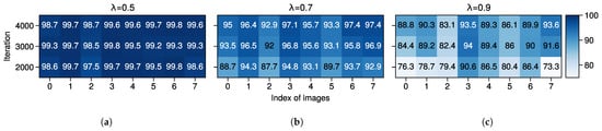
Figure 8. $P_{\mathsf{h}}$: Percentage (%) of high-quality pseudo-labels with different threshold $\lambda$ on POT→VAI, calculated from eight randomly selected images. (a) $\lambda$ = 0.5. (b) $\lambda$ = 0.7. (c) $\lambda$ = 0.9.

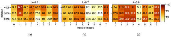
Figure 9. $P_{\mathsf{c}}$: Percentage of correct ones in $P_{\mathsf{h}}$ with different threshold $\lambda$ on POT→VAI, calculated from the same images in Figure 8. (a) $\lambda$ = 0.5. (b) $\lambda$ = 0.7. (c) $\lambda$ = 0.9.

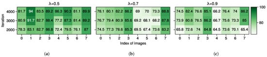
Figure 10. $P_{\mathsf{ch}}$: Percentage (%) of correct high-quality pseudo-labels with different threshold $\lambda$ on POT→VAI, calculated from the same images in Figure 8. (a) $\lambda$ = 0.5. (b) $\lambda$ = 0.7. (c) $\lambda$ = 0.9.

As shown in Figure 8, the results are per our intuitions: (1) the larger the pseudo-label threshold is, the more strict the LDQ will become, and (2) the more iterations the model learns, the more confident it will become in the target domain. Note that the word “strict” describes the strength of the criteria for determining the quality of pseudo-labels, regardless of their correctness. In Figure 9, with the largest threshold $\lambda =0.9$, most of the generated pseudo-labels $p_T$ are more accurate and trustworthy compared to the results when $\lambda =0.5$ except for images 1 and 4. However, with the iteration of the training stage, the correct ratio $P_{\mathsf{c}}$ of some pseudo-labels even decreases, e.g., image 4 in Figure 9b and images 2 and 3 in Figure 9. These results are reasonable since it is challenging to determine whether the generated pseudo-labels are high-quality merely by a threshold value $\lambda$. The results of $P_{\mathsf{ch}}$ are shown in Figure 10, which indicates the ratio of correct pseudo-labels practically learned by our model. According to the results, the model learns the maximum proportion of correct pseudo-labels when $\lambda =0.5$ among these images. The accuracy of pseudo-labels is highest overall when the $\lambda =0.9$, as shown in Figure 9c. The least high-quality pseudo-labels are generated in Figure 10c, resulting in a low proportion of correct pseudo-labels learned by the model. This suggests that during the adaptation from POT to VAI, samples with confidence slightly above 0.5 are mostly correct, while those with particularly high confidence are the least correct. We believe that the presence of some features with the same distribution but different categories in the two datasets, i.e., domain gaps, seriously misleads the model. In summary, a larger threshold $\lambda$ model generates pseudo-labels with higher accuracy, but it might limit the number of high-quality pseudo-labels, both of which require some trade-off in use. A larger threshold $\lambda$ induces the model to predict more accurate but fewer high-quality pseudo-labels, so there is a trade-off between accuracy and quantity.

We investigate the effect of K by analyzing the mean quality of the correct and incorrect pseudo-labels calculated through Equation (7). Similarly, these experiments are conducted with different K but the same pseudo-labels’ threshold $\lambda =0.7$, and the results are shown in Figure 11 and Figure 12. The quantitative performance can be found in Table A2 in Appendix A. In the case of $K=2,3$, and 4, the average quality of incorrect pseudo-labels is reduced by 11.91%, 11.07%, and 19.14%, respectively, compared to the correct ones at iteration 4000. In comparison to the image-wise quality [28,30], our strategy improved the quality of pseudo-labels with very little overhead. As for the values of K, it is suggested to pick a proper K to ensure that $2K+1$ is below the width of the minimal segmentation target since the data near the boundary are harder to classify and usually get lower confidence.

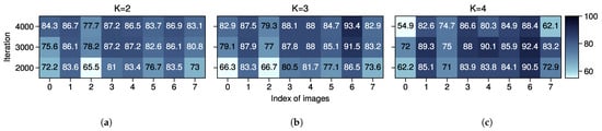
Figure 11. Averaged quality (%) of incorrect pseudo-labels with different K on POT→VAI, calculated from the same images in Figure 8. (a) K = 2. (b) K = 3. (c) K = 4.

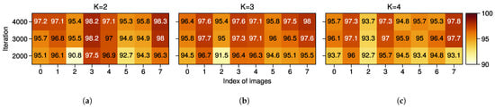
Figure 12. Averaged quality (%) of correct pseudo-labels with different K on POT→VAI, calculated from the same images in Figure 8. (a) K = 2. (b) K = 3. (c) K = 4.

4.3. Computational Complex Analysis

In this paper, the number of all parameters for the DAFormer [30] with MiT-B5 encoder [6] is 85.15 M, compared to 62.7 M for DeepLabV3+ [4]. Although the vision Transformer is larger than CNNs, no auxiliary networks are needed in the self-training framework, so there is no other overhead. For example, the generative-based network structure of ResiDualGAN [23] contains two generators and two discriminators, each with 41.82 M and 6.96 M parameters, respectively. Each generator and discriminator has 41.82 M and 6.96 M parameters, respectively, for a total of 97.56 M parameters. As a result, the computational complexity of our method is completely acceptable.

4.4. Limitations

We have verified the effectiveness of the Transformer and proposed GCW and LDQ in UDA for semantic segmentation of RS images. However, there are many unsolved and unexplored issues in our proposed framework. Due to computational constraints, only one type of Transformer with limited iterations has been tested to support our claims. The potential of the vision Transformer in UDA of RS semantic segmentation could be explored in further studies using network architectures such as those proposed in [5,6,7,8].

Hoyer et al. [30] demonstrated that Transformer outperforms most previous UDA methods using DeepLabV2 [29] or DeepLabV3+ [4]. However, their experiments are based on pre-training and large datasets, which are difficult to achieve in the field of remote sensing. While adapting to a large dataset from a tiny dataset, there might be insufficient data and features available for the elaborate Transformer to learn, which thus derives some inferior and unstable performance. For example, the overall performance on the POT→VAI is better than on VAI→POT since there is more training data in POT. Additionally, the IoU for the clutter category on VAI→POT is close to 0. Therefore, further studies are required to facilitate improvements in the UDA performance with Transformers on small datasets.

In Figure 6, the values of GCW fluctuate at the beginning but eventually become steady. Accordingly, the model does not gain significant additional performance in later iterations but only retrains the advantages obtained in the early stages. The GCW formula could be changed in subsequent iterations to improve domain adaptation to the target domain.

The LDQ is based on the assumption that the model predicts with low confidence for incorrect predictions while producing high confidence for correct predictions. However, it may break down in some cases, such as the domain adaptation between two domains with particularly large gaps. As illustrated in Table 1 and Table 2, the performance with LDQ degrades in some classes compared to the baseline. For instance, the IoU of the car class reduces by 2.91% on POT→VAI, while it decreased from 41.98% to 6.91% on VAI→POT in the vegetation class. Since the results become much more feasible by combining GCW and LDQ, it is suggested to use LDQ with robust strategies for better performance.

5. Conclusions

In this article, we reveal the remarkable potential of the vision Transformer for the task of unsupervised domain adaptation for remote sensing image-semantic segmentation. Additionally, Gradual Class Weights (GCW) and Local Dynamic Quality (LDQ), two simple but effective training strategies working on the source and target domains, respectively, are introduced to stabilize and boost the performance of UDA. Compared to other UDA methods for RS image-semantic segmentation using DeepLabV3+ [4], our method improves the state-of-the-art performance by 8.23% mIoU on POT→VAI and 9.2% mIoU on VAI→POT. Notably, GCW improved the performance by addressing the class imbalance problem and allowing healthy convergence at the beginning of the training stage. In addition, LDQ serves by reducing and increasing the weights of the incorrect and correct pseudo-labels, respectively. The two strategies can be effortlessly embedded in various types of semantic segmentation domain-adaptation methods to boost performance. Furthermore, our strategies enable the model to learn even the difficult classes such as clutter/background. In our future work, we will focus on improving UDA performance with Transformers on small datasets.

References

- Long, J.; Shelhamer, E.; Darrell, T. Fully convolutional networks for semantic segmentation. In Proceedings of the IEEE Conference on Computer Vision and Pattern Recognition, Boston, MA, USA, 7–12 June 2015; pp. 3431–3440. [Google Scholar]
- Ronneberger, O.; Fischer, P.; Brox, T. U-net: Convolutional networks for biomedical image segmentation. In Proceedings of the International Conference on Medical Image Computing and Computer-Assisted Intervention, Munich, Germany, 5–9 October 2015; Springer: Berlin/Heidelberg, Germany, 2015; pp. 234–241. [Google Scholar]
- Zhao, H.; Shi, J.; Qi, X.; Wang, X.; Jia, J. Pyramid scene parsing network. In Proceedings of the IEEE Conference on Computer Vision and Pattern Recognition, Honolulu, HI, USA, 21–26 July 2017; pp. 2881–2890. [Google Scholar]
- Chen, L.C.; Zhu, Y.; Papandreou, G.; Schroff, F.; Adam, H. Encoder-decoder with atrous separable convolution for semantic image segmentation. In Proceedings of the European Conference on Computer Vision (ECCV), Munich, Germany, 8–14 September 2018; pp. 801–818. [Google Scholar]
- Zheng, S.; Lu, J.; Zhao, H.; Zhu, X.; Luo, Z.; Wang, Y.; Fu, Y.; Feng, J.; Xiang, T.; Torr, P.H.; et al. Rethinking semantic segmentation from a sequence-to-sequence perspective with transformers. In Proceedings of the IEEE/CVF Conference on Computer Vision and Pattern Recognition, Nashville, TN, USA, 20–25 June 2021; pp. 6881–6890. [Google Scholar]
- Xie, E.; Wang, W.; Yu, Z.; Anandkumar, A.; Alvarez, J.M.; Luo, P. SegFormer: Simple and efficient design for semantic segmentation with transformers. Adv. Neural Inf. Process. Syst. 2021, 34, 12077–12090. [Google Scholar]
- Xu, Z.; Zhang, W.; Zhang, T.; Yang, Z.; Li, J. Efficient transformer for remote sensing image segmentation. Remote Sens. 2021, 13, 3585. [Google Scholar] [CrossRef]
- Zhang, P.; Zhang, B.; Zhang, T.; Chen, D.; Wang, Y.; Wen, F. Prototypical Pseudo Label Denoising and Target Structure Learning for Domain Adaptive Semantic Segmentation. arXiv 2021, arXiv:2101.10979. [Google Scholar]
- Toldo, M.; Maracani, A.; Michieli, U.; Zanuttigh, P. Unsupervised domain adaptation in semantic segmentation: A review. Technologies 2020, 8, 35. [Google Scholar] [CrossRef]
- Yang, Y.; Soatto, S. Fda: Fourier domain adaptation for semantic segmentation. In Proceedings of the IEEE/CVF Conference on Computer Vision and Pattern Recognition, Seattle, WA, USA, 13–19 June 2020; pp. 4085–4095. [Google Scholar]
- Ma, H.; Lin, X.; Wu, Z.; Yu, Y. Coarse-to-fine domain adaptive semantic segmentation with photometric alignment and category-center regularization. In Proceedings of the IEEE/CVF Conference on Computer Vision and Pattern Recognition, Nashville, TN, USA, 20–25 June 2021; pp. 4051–4060. [Google Scholar]
- Tuia, D.; Munoz-Mari, J.; Gomez-Chova, L.; Malo, J. Graph matching for adaptation in remote sensing. IEEE Trans. Geosci. Remote Sens. 2012, 51, 329–341. [Google Scholar] [CrossRef]
- Rakwatin, P.; Takeuchi, W.; Yasuoka, Y. Restoration of Aqua MODIS band 6 using histogram matching and local least squares fitting. IEEE Trans. Geosci. Remote Sens. 2008, 47, 613–627. [Google Scholar] [CrossRef]
- Goodfellow, I.; Pouget-Abadie, J.; Mirza, M.; Xu, B.; Warde-Farley, D.; Ozair, S.; Courville, A.; Bengio, Y. Generative adversarial networks. Commun. ACM 2020, 63, 139–144. [Google Scholar] [CrossRef]
- Yi, Z.; Zhang, H.; Tan, P.; Gong, M. Dualgan: Unsupervised dual learning for image-to-image translation. In Proceedings of the IEEE International Conference on Computer Vision, Venice, Italy, 22–29 October 2017; pp. 2849–2857. [Google Scholar]
- Zhu, J.Y.; Park, T.; Isola, P.; Efros, A.A. Unpaired image-to-image translation using cycle-consistent adversarial networks. In Proceedings of the IEEE International Conference on Computer Vision, Venice, Italy, 22–29 October 2017; pp. 2223–2232. [Google Scholar]
- Hoffman, J.; Tzeng, E.; Park, T.; Zhu, J.Y.; Isola, P.; Saenko, K.; Efros, A.; Darrell, T. Cycada: Cycle-consistent adversarial domain adaptation. In Proceedings of the International Conference on Machine Learning, Stockholm, Sweden, 10–15 July 2018; pp. 1989–1998. [Google Scholar]
- Benjdira, B.; Bazi, Y.; Koubaa, A.; Ouni, K. Unsupervised domain adaptation using generative adversarial networks for semantic segmentation of aerial images. Remote Sens. 2019, 11, 1369. [Google Scholar] [CrossRef]
- Tsai, Y.H.; Hung, W.C.; Schulter, S.; Sohn, K.; Yang, M.H.; Chandraker, M. Learning to adapt structured output space for semantic segmentation. In Proceedings of the IEEE Conference on Computer Vision and Pattern Recognition, Salt Lake City, UT, USA, 18–23 June 2018; pp. 7472–7481. [Google Scholar]
- Li, Y.; Shi, T.; Zhang, Y.; Chen, W.; Wang, Z.; Li, H. Learning deep semantic segmentation network under multiple weakly-supervised constraints for cross-domain remote sensing image semantic segmentation. ISPRS J. Photogramm. Remote Sens. 2021, 175, 20–33. [Google Scholar] [CrossRef]
- Cai, Y.; Yang, Y.; Zheng, Q.; Shen, Z.; Shang, Y.; Yin, J.; Shi, Z. BiFDANet: Unsupervised Bidirectional Domain Adaptation for Semantic Segmentation of Remote Sensing Images. Remote Sens. 2022, 14, 190. [Google Scholar] [CrossRef]
- Gao, H.; Zhao, Y.; Guo, P.; Sun, Z.; Chen, X.; Tang, Y. Cycle and Self-Supervised Consistency Training for Adapting Semantic Segmentation of Aerial Images. Remote Sens. 2022, 14, 1527. [Google Scholar] [CrossRef]
- Zhao, Y.; Gao, H.; Guo, P.; Sun, Z. ResiDualGAN: Resize-Residual DualGAN for Cross-Domain Remote Sensing Images Semantic Segmentation. arXiv 2022, arXiv:2201.11523. [Google Scholar]
- Vu, T.H.; Jain, H.; Bucher, M.; Cord, M.; Pérez, P. Advent: Adversarial entropy minimization for domain adaptation in semantic segmentation. In Proceedings of the IEEE/CVF Conference on Computer Vision and Pattern Recognition, Long Beach, CA, USA, 16–17 June 2019; pp. 2517–2526. [Google Scholar]
- Zou, Y.; Yu, Z.; Kumar, B.; Wang, J. Unsupervised domain adaptation for semantic segmentation via class-balanced self-training. In Proceedings of the European Conference on Computer Vision (ECCV), Munich, Germany, 8–14 September 2018; pp. 289–305. [Google Scholar]
- Yan, L.; Fan, B.; Xiang, S.; Pan, C. CMT: Cross Mean Teacher Unsupervised Domain Adaptation for VHR Image Semantic Segmentation. IEEE Geosci. Remote Sens. Lett. 2021, 19, 1–5. [Google Scholar] [CrossRef]
- Olsson, V.; Tranheden, W.; Pinto, J.; Svensson, L. Classmix: Segmentation-based data augmentation for semi-supervised learning. In Proceedings of the IEEE/CVF Winter Conference on Applications of Computer Vision, Waikoloa, HI, USA, 4–8 January 2021; pp. 1369–1378. [Google Scholar]
- Tranheden, W.; Olsson, V.; Pinto, J.; Svensson, L. Dacs: Domain adaptation via cross-domain mixed sampling. In Proceedings of the IEEE/CVF Winter Conference on Applications of Computer Vision, Waikoloa, HI, USA, 4–8 January 2021; pp. 1379–1389. [Google Scholar]
- Chen, L.C.; Papandreou, G.; Kokkinos, I.; Murphy, K.; Yuille, A.L. Deeplab: Semantic image segmentation with deep convolutional nets, atrous convolution, and fully connected crfs. IEEE Trans. Pattern Anal. Mach. Intell. 2017, 40, 834–848. [Google Scholar] [CrossRef]
- Hoyer, L.; Dai, D.; Van Gool, L. Daformer: Improving network architectures and training strategies for domain-adaptive semantic segmentation. In Proceedings of the IEEE/CVF Conference on Computer Vision and Pattern Recognition, New Orleans, LA, USA, 21–24 June 2022; pp. 9924–9935. [Google Scholar]
- Zhang, H.; Cisse, M.; Dauphin, Y.N.; Lopez-Paz, D. mixup: Beyond empirical risk minimization. arXiv 2017, arXiv:1710.09412. [Google Scholar]
- Yun, S.; Han, D.; Oh, S.J.; Chun, S.; Choe, J.; Yoo, Y. Cutmix: Regularization strategy to train strong classifiers with localizable features. In Proceedings of the IEEE/CVF International Conference on Computer Vision, Seoul, Korea, 27 October–2 November 2019; pp. 6023–6032. [Google Scholar]
- Chen, T.; Kornblith, S.; Norouzi, M.; Hinton, G. A simple framework for contrastive learning of visual representations. In Proceedings of the International Conference on Machine Learning, Virtual, 13–18 July 2020; pp. 1597–1607. [Google Scholar]
- Haixiang, G.; Yijing, L.; Shang, J.; Mingyun, G.; Yuanyue, H.; Bing, G. Learning from class-imbalanced data: Review of methods and applications. Expert Syst. Appl. 2017, 73, 220–239. [Google Scholar] [CrossRef]
- Yan, H.; Ding, Y.; Li, P.; Wang, Q.; Xu, Y.; Zuo, W. Mind the class weight bias: Weighted maximum mean discrepancy for unsupervised domain adaptation. In Proceedings of the IEEE Conference on Computer Vision and Pattern Recognition, Honolulu, HI, USA, 21–26 July 2017; pp. 2272–2281. [Google Scholar]
- Zeiler, M.D.; Fergus, R. Visualizing and understanding convolutional networks. In Proceedings of the European Conference on Computer Vision, Zurich, Switzerland, 6–12 September 2014; Springer: Berlin/Heidelberg, Germany, 2014; pp. 818–833. [Google Scholar]
- Olah, C.; Mordvintsev, A.; Schubert, L. Feature Visualization. Distill 2017, 2, e7. [Google Scholar] [CrossRef]
- Goyal, P.; Dollár, P.; Girshick, R.; Noordhuis, P.; Wesolowski, L.; Kyrola, A.; Tulloch, A.; Jia, Y.; He, K. Accurate, large minibatch sgd: Training imagenet in 1 hour. arXiv 2017, arXiv:1706.02677. [Google Scholar]
- International Society for Photogrammetry and Remote Sensing. 2D Semantic Labeling Contest-Potsdam. Available online: https://www.isprs.org/education/benchmarks/UrbanSemLab/2d-sem-label-potsdam.aspx (accessed on 21 August 2022).
- International Society for Photogrammetry and Remote Sensing. 2D Semantic Labeling Contest-Vaihingen. Available online: https://www.isprs.org/education/benchmarks/UrbanSemLab/2d-sem-label-vaihingen.aspx (accessed on 21 August 2022).
- Paszke, A.; Gross, S.; Massa, F.; Lerer, A.; Bradbury, J.; Chanan, G.; Killeen, T.; Lin, Z.; Gimelshein, N.; Antiga, L.; et al. PyTorch: An Imperative Style, High-Performance Deep Learning Library. In Advances in Neural Information Processing Systems 32; Wallach, H., Larochelle, H., Beygelzimer, A., d’Alché-Buc, F., Fox, E., Garnett, R., Eds.; Curran Associates, Inc.: Vancouver, BC, Canada, 2019; pp. 8024–8035. [Google Scholar]
- Contributors, M. MMSegmentation: OpenMMLab Semantic Segmentation Toolbox and Benchmark. 2020. Available online: https://github.com/open-mmlab/mmsegmentation (accessed on 21 August 2022).
- Deng, J.; Dong, W.; Socher, R.; Li, L.J.; Li, K.; Fei-Fei, L. ImageNet: A large-scale hierarchical image database. In Proceedings of the 2009 IEEE Conference on Computer Vision and Pattern Recognition, Miami, FL, USA, 20–25 June 2009; pp. 248–255. [Google Scholar] [CrossRef]
- Mehta, S.; Rastegari, M.; Shapiro, L.; Hajishirzi, H. Espnetv2: A light-weight, power efficient, and general purpose convolutional neural network. In Proceedings of the IEEE/CVF Conference on Computer Vision and Pattern Recognition, Long Beach, CA, USA, 15–20 June 2019; pp. 9190–9200. [Google Scholar]
- Loshchilov, I.; Hutter, F. Decoupled weight decay regularization. arXiv 2017, arXiv:1711.05101. [Google Scholar]
Publisher’s Note: MDPI stays neutral with regard to jurisdictional claims in published maps and institutional affiliations. |
© 2022 by the authors. Licensee MDPI, Basel, Switzerland. This article is an open access article distributed under the terms and conditions of the Creative Commons Attribution (CC BY) license (https://creativecommons.org/licenses/by/4.0/).