Abstract
Very shallow coral reefs (<5 m deep) are naturally exposed to strong sea surface temperature variations, UV radiation and other stressors exacerbated by climate change, raising great concern over their future. As such, accurate and ecologically informative coral reef maps are fundamental for their management and conservation. Since traditional mapping and monitoring methods fall short in very shallow habitats, shallow reefs are increasingly mapped with Unmanned Aerial Vehicles (UAVs). UAV imagery is commonly processed with Structure-from-Motion (SfM) to create orthomosaics and Digital Elevation Models (DEMs) spanning several hundred metres. Techniques to convert these SfM products into ecologically relevant habitat maps are still relatively underdeveloped. Here, we demonstrate that incorporating geomorphometric variables (derived from the DEM) in addition to spectral information (derived from the orthomosaic) can greatly enhance the accuracy of automatic habitat classification. Therefore, we mapped three very shallow reef areas off KAUST on the Saudi Arabian Red Sea coast with an RTK-ready UAV. Imagery was processed with SfM and classified through object-based image analysis (OBIA). Within our OBIA workflow, we observed overall accuracy increases of up to 11% when training a Random Forest classifier on both spectral and geomorphometric variables as opposed to traditional methods that only use spectral information. Our work highlights the potential of incorporating a UAV’s DEM in OBIA for benthic habitat mapping, a promising but still scarcely exploited asset.
1. Introduction
Coral reefs are well known for the high biodiversity they support, but also for their susceptibility to anthropogenic pressures and climate change-derived environmental modifications [1]. Increasing sea surface temperatures, in particular, have proven highly detrimental to coral reefs, as they can trigger coral bleaching events in which the coral hosts lose their symbiotic algae, often resulting in coral mortality [1,2,3]. Coral bleaching events disproportionately affect very shallow coral reefs (<5 m deep), because they are naturally exposed to greater temperature variations [3,4,5]. To counteract the effects of these stressors and support the survival of coral reef ecosystems in the coming decades, ecosystem-based management has been widely advocated within the scientific community [6,7,8,9]. A crucial part of ecosystem-based management is understanding and dealing with spatial heterogeneity, for example, through marine spatial planning [10,11]. Marine habitat mapping has therefore been identified as a key foundation of ecosystem-based management [12,13,14]. As such, there is a great need for accurate and ecologically informative maps of shallow coral reefs.
Coral reefs are typically located in shallow, tropical, oligotrophic waters. In such environments, boat-based acoustic mapping methods struggle, but monitoring the spatial distribution of benthic assemblages with aerial imagery is effective [15,16,17,18]. At a large scale (regional–world), satellite imagery can be used to map coral reefs. However, as the spatial resolution offered by satellites is relatively coarse, they are not always able to distinguish features of ecological importance [15,17,18,19]. To overcome these limitations, planes are occasionally deployed to collect aerial images at higher spatial resolutions, but their deployment can be prohibitively expensive [15,18,20]. Unmanned Aerial Vehicles (UAVs) or ‘drones’ are also able to capture spatial data at very high spatial resolutions and offer great flexibility in their deployment for only a fraction of the costs, making them an effective surveying tool [15,17,18,21]. Consequently, the use of UAVs to map shallow coral reefs has taken flight in recent years [22,23,24,25,26,27,28,29,30].
To maximise the surveying potential of UAVs, hundreds of UAV images are typically combined into a single orthomosaic of high spatial resolution with Structure-from-Motion (SfM) algorithms [25,29,31]. SfM processing simultaneously provides the user with reconstructions of the three-dimensional structure of the mapped area in the form of a point cloud and a Digital Elevation Model (DEM) [29,31,32]. As three-dimensional structure and water depth are instrumental to ecosystem functioning on coral reefs, such information is of great ecological value [3,33]. Underwater SfM has, for instance, been used to quantify the contribution of different coral taxa to reef structural complexity [32,34,35]. UAV-derived DEMs, on the other hand, can be used to quantify variation in the three-dimensional structure at the reef scale, allowing Fallati et al. [22] to detect a reduction in reef rugosity after a coral bleaching event in the Maldives.
To truly benefit ecosystem-based management, UAV data must be converted into easily interpretable and ecologically relevant habitat maps [12,13,14,15,36]. Techniques to automatically convert UAV data into habitat maps are still in their infancy. Habitat mapping efforts using satellite imagery have been around for much longer. Due to ever-increasing image resolutions, this field has undergone a paradigm shift from pixel-based approaches to Object-Based Image Analysis (OBIA) in recent decades [37,38]. Central to OBIA is the segmentation of an image into distinct regions based on homogeneity criteria before classification. Creating such ‘image objects’ allows the extraction of not only spectral, but also structural, contextual, and spatial information from the image, significantly improving image classification results compared to pixel-based approaches [37,38,39]. The high spatial resolution of UAV-derived orthomosaics makes them particularly suitable for classification through OBIA. Consequently, OBIA has been successfully used in the marine environment to classify UAV orthomosaics of various habitats, e.g., a seagrass meadow, a rocky coast, a Sabellaria worm reef, and two shallow coral reefs [22,40,41].
Despite the simultaneous presentation of SfM analyses and OBIA, to the best of our knowledge, no research has tested the effect of incorporating a UAV-derived DEM into OBIA in the marine environment yet. Meanwhile, in terrestrial habitats, combining geomorphometric parameters and spectral variables in OBIA has proven to be a successful approach [42,43,44,45,46]. Low spatial resolution (>1 m/pixel) DEMs have, for instance, been combined with satellite imagery to improve classifications of agricultural areas in Spain and Madagascar or with aerial imagery to successfully map coastal vegetation in Denmark [43,45,46]. Moreover, two UAV-based studies showed that high-resolution (<1 m/pixel) SfM-derived DEMs can be used to improve automatic classification of a glacier and a sugarcane field, respectively [42,44]. Here, we demonstrate that despite the challenges of SfM analyses in the marine environment [18,25,30], integrating an SfM-derived DEM into OBIA is also a viable approach for creating accurate and ecologically relevant habitat maps in shallow tropical marine habitats. We specifically investigated three uses of UAV-derived geomorphometric variables to improve tropical marine habitat classification: (1) we investigated whether the DEM could be used to semantically delineate a reef’s geomorphological zones, e.g., the reef slope and the reef flat [47,48]; (2) we tested whether performing the automatic habitat classification separately in each of these reef zones increased classification accuracy by constraining the effects of depth-related light attenuation [48,49,50]; and (3) we studied whether incorporating UAV-derived geomorphometric variables into the automatic habitat classification with a Random Forest algorithm increased mapping accuracy [33,42,43,44,45,46]. To that end, three very shallow reef areas in a lagoon in the central Saudi Arabian Red Sea were surveyed, resulting in three multi-layered, ecologically informative habitat maps of the local reef shallows.
2. Materials and Methods
2.1. Study Area
Data collection took place on 16 December 2021 and 8–9 February 2022 in a coastal lagoon within the campus of the King Abdullah University of Science and Technology (KAUST), situated north of the town of Thuwal in Saudi Arabia (~22.28° N, 39.10° E, Figure 1). This ~2.3 km2 lagoon is shielded from the Red Sea by a fringing reef and consists of a combination of sand flats, seagrass, and reef patches. The edges of the lagoon are occupied by mangroves and to the southeast, the lagoon is connected to a channel running through KAUST’s campus. Inside the lagoon, two shallow areas were mapped that showed promising reef patches on satellite imagery. Additionally, a narrow stroke of exposed fringing reef at the lagoon’s entrance was mapped (Figure 1). Located within the campus, the lagoon has likely been exposed to considerable anthropogenic pressures throughout the past fifteen years, especially during KAUST’s construction from 2007 to 2009. In addition, shallow inshore reefs in this region suffered substantially from the global coral bleaching events of 2010 and 2015/2016 [4,5]. As coastal development in Saudi Arabia is quickly expanding and global temperatures continue to rise, many reefs along the Saudi Arabian Red Sea may be exposed to similar pressures in the near future [51]. Thus, the areas mapped here present a good case study for the Red Sea reefs of the future.
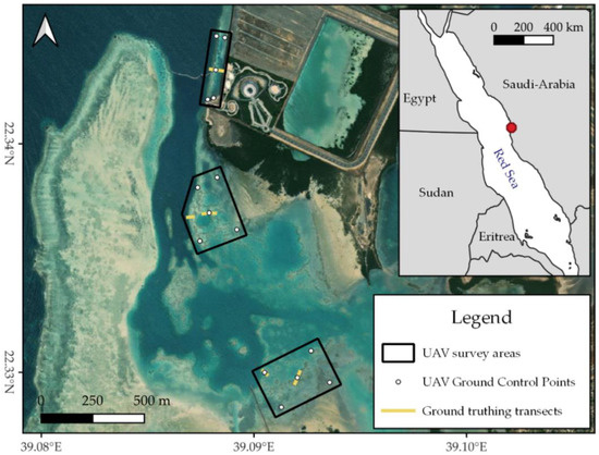
Figure 1.
Map indicating the study areas in the KAUST lagoon. The white numbers are used to differentiate between the three survey areas. Inset indicates the general location of the KAUST lagoon on the Saudi Arabian Red Sea coast. Map contains ESRI World Imagery and Natural Earth data. All maps in this work were created with QGIS v.3.22.
2.2. Aerial Data Collection
Very shallow reef areas (<5 m deep) were surveyed with a DIJ Phantom 4 Pro RTK. The Phantom 4 Pro RTK comes equipped with a 1-inch CMOS camera sensor (5472 × 3648 pixels) that takes true colour images (RGB) through an 8.8 mm (24 mm Full Frame equivalent) lens, mounted on an integrated gimbal [52]. A Nisi polarising filter was added to the lens to minimise glint. In addition, the Phantom 4 RTK is standardly fitted with a dual-frequency GNSS unit that records raw satellite navigation data in a RINEX 3.03 format. This allows users to record the geolocation of the UAV’s pictures with centimetre-level accuracy through either Real-Time Kinematics (RTK) or Post-Processed Kinematics (PPK) [52].
Flight plans were designed using the DJI GS RTK app. To minimise glint and wave distortion, UAV flights were planned within the first four hours after sunrise on days with little wind (<2.5 m/s). The tidal stage was not taken into account when planning field surveys, as tides are minimal in this region (tidal range <0.5 m) [53]. During image acquisition, the UAV followed a lawnmower pattern at an altitude of 40 m with the camera oriented at nadir, resulting in a ground sampling resolution of ~1.1 cm/pixel (Table 1). To ensure motion blur was absent, the shutter speed was fixed at 1/640 s while flying at a speed of only 2.0 m/s (Table 1). Flying at these speeds allowed a frontal overlap of 90% between pictures (within flight lines). The lateral overlap between flight lines was set to 75% balancing flight time and SfM quality (Table 1) [18]. To improve the vertical accuracy of SfM outputs and overcome the ‘doming effect’, a small set of oblique imagery was acquired at the end of each flight via the ‘altitude optimization’ option in the DJI GS RTK app [54,55,56] (Table 1).

Table 1.
Aerial image acquisition settings used during all UAV surveys. Any setting not explicitly mentioned here was kept at default.
Combining RTK/PPK positioning of the UAV with a few Ground Control Points (GCPs) has been shown to mitigate the systematic vertical error sometimes associated with PPK-only surveys [56,57,58,59]. Additionally, using underwater GCPs was shown to be the most useful method to correct for the effects of refraction when processing UAV imagery of shallow marine habitats with SfM algorithms [25]. Thus, at every survey location, five highly visible markers were installed underwater as GCPs. One GCP was placed in each corner and one in the middle (Figure 1). The exact location of each GCP was measured with a dual-frequency Emlid Reach RS2 RTK GNSS. This GNSS was controlled via Emlid’s ReachView 3 v6.13 mobile app and set to record raw RINEX 3.03 data in kinematic mode with a sampling rate of 10 Hz. At each GCP, the GNSS was held still for 60 s to create a recognisable cloud of points in the track.
2.3. PPK Geolocation of UAV Images and GCPs
UAV pictures and GCPs were geolocated with centimetre-level accuracy with a PPK workflow as presented by Taddia et al. [56]. Briefly, a PPK workflow uses the raw satellite navigation data recorded by a GNSS receiver and compares them to the raw satellite data recorded by a second receiver at a known location. By comparing the change in satellite positions between the two GNSS receivers, the algorithm is able to reconstruct the location of the first receiver with centimetre-level accuracy [60].
In this study, the receiver at an unknown location is either represented by the Phantom 4 RTK or, in the case of the GCPs, by the Emlid Reach RS2. In both cases, the receiver providing PPK corrections was the KSA-CORS network’s MK96 receiver (22.28051° N, 39.113477° E) [61]. PPK of UAV images was performed in REDtoolbox v2.82 by REDcatch GmhB. This software first performs PPK on the UAV’s navigation data and then extracts the exact coordinates of each UAV image using its timestamp. Subsequently, a copy of each image is created with the new location, including its accuracy, stored in the EXIF data [62]. To post-process the location of the GCPs, we used Emlid Studio v1.10, which is based on the open-source software RTKLIB. After PPK processing, the resulting .pos file was inspected in Emlid Studio and the coordinates of the GCPs were manually extracted from the most central point in the point cloud of each GCP.
2.4. Ground Truth Data Collection
To gather ground truth data for the UAV surveys, underwater pictures were collected during snorkelling transects. In each survey area, at least two 30-metre transects were conducted, starting from the middle UAV GCP (Figure 1). For the two areas inside the lagoon, an extra transect was added to make sure underwater imagery also covered the reef slope, where the benthic community changed quickly to a community dominated by live coral (Figure 1, personal observation B.O.N.). To maximise the spatial accuracy of the ground truth data, underwater imagery—where possible—was processed with SfM and geolocated with GCPs, which were placed along the transects at five-metre intervals. Their exact location was recorded in the same way as described for the UAV’s GCPs. A more detailed description of underwater image acquisition is available in the Supplementary Materials (Section S1).
2.5. Structure-from-Motion Processing
Both our underwater and UAV picture collections were processed with Structure-from-Motion algorithms following the general methods as explained by Westoby et al. [31]. Nowadays, multiple types of commercial software are available that can generate 3D point clouds, 3D mesh models, Digital Elevation Models (DEMs), and orthomosaics from a set of pictures using SfM algorithms. Our UAV imagery was processed with Pix4Dmapper v4.6.4 by Pix4D, which was chosen over other software because Pix4Dmapper automatically reads the geotags and their accuracies as stored in the image EXIF data by REDtoolbox, thus offering a smooth PPK-SfM workflow. Moreover, despite contrasting results in the past, a recent study showed that in comparison to other software, Pix4D generates the most accurate output when processing UAV images [63,64]. Underwater pictures were processed in Agisoft Metashape Professional 1.7.5 by Agisoft LLC., which was preferred over Pix4D because it was much better at aligning the non-georeferenced underwater images correctly in our relatively long underwater transects; similar observations were made by Burns and Delparte [65]. An exhaustive protocol of our SfM processing of both UAV and underwater imagery can be found in the Supplementary Materials (Section S2).
2.6. Geomorphometric Variables
After SfM processing, a geomorphometric analysis was performed in SAGA (System for Automated Geoscientific Analysis) v7.9.0 on the UAV-derived DEMs [66]. To reduce SfM processing noise, all DEMs were resampled to a resolution of 1.5 cm per pixel and filtered with the Gaussian filter (radius = 15 cm). A constant transformation of −5.58 m was applied to convert the DEM raster values from WGS 84 ellipsoidal height to orthometric elevation in relation to the KSA-GEOID2017 [67,68]. Subsequently, several geomorphometric variables were calculated from the filtered and transformed DEMs. We calculated the Multi-Scale Topographic Position Index (TPI), slope, aspect, vector ruggedness (VRM), and profile curvature [69,70,71,72]. Multi-Scale TPI was calculated in a range of 45–150 cm, which resembles the size range of reef outcrops. VRM was calculated in a radius of 5.25 cm to show fine-scale rugosity. A correlation matrix—constructed from ≥100 randomly extracted raster values—was used to ensure that all geomorphometric variables provided independent data (Supplementary Material Figures S3–S5).
2.7. Habitat Classification through Object-Based Image Analysis
Habitat classification was performed in eCognition Developer v10.0.1 by Trimble Germany GmbH, following an Object-Based Image Analysis (OBIA) workflow [37,73]. In short, OBIA is an image classification approach that groups image pixels into distinct segments—so-called ‘image objects’—before classification based on their (spectral) homogeneity. This is particularly useful for high-resolution image data in which single pixels are spectrally indiscriminate and do not resemble meaningful real-life objects [37,38]. More importantly, the creation of image objects opens up the possibility to extract not only spectral information, but also statistical, structural, spatial, and contextual information [37,39]. For example, an image object has an average brightness, a standard deviation in brightness, a shape, an area, and a location. Furthermore, image objects have a defined relation (e.g., neighbour) to other image objects, including hierarchical relations with sub- or super-objects [39,73]. All this extra information can be employed during the subsequent habitat classification, severely improving classification accuracy and information content of the final classification compared to pixel-based approaches [37,38,39].
In our classification protocol, we first delineated the area of interest by dividing each survey area into three categories: deep water, shallow water, and land. Employing eCognition’s ‘multi-threshold segmentation’ algorithm on the filtered DEM, everything deeper than 3.5 m was classified as deep water, 3.5–0 m deep was classified as shallow water, and everything above 0 m was classified as land [73]. Because we were mainly interested in the real water conditions at the time of sampling, this classification was fine-tuned by subtracting the average altitude of the water’s edge as visible in the orthomosaic. A minimum object size of 800,000 pixels ensured that only large regions were delineated and not, for instance, floating seaweed patches. Using similar methods, our area of interest, shallow water, was subdivided into three geomorphological zones: the reef slope (1–3.5 m deep), the deep reef flat (1–3.5 m deep), and the shallow reef flat (<1 m deep) [47,74]. The reef slope was identified as any area deeper than 1 m that bordered ‘deep water’. All other areas deeper than 1 m were classified as ‘the deep reef flat’ and all areas shallower than 1 m as ‘the shallow reef flat’.
The reef slope and reef flat were then subjected to the ‘multiresolution segmentation’ algorithm. This algorithm divides an image into a set of ‘image objects’ (distinct segments) by consecutively merging previously created image objects starting at the pixel level. While doing so, the algorithm aims to minimise the heterogeneity of the resulting image objects. For this heterogeneity criterion, the algorithm considers both the shape and spectral properties of the image objects. The algorithm continues to merge objects until a predetermined heterogeneity threshold is reached [39,73]. In our analysis, this segmentation was based on the RGB bands from the orthomosaic only. The relative weight of the shape criterion was set to 0.1, resulting in a relative weight of 0.9 for spectral values. Compactness and smoothness criteria were given an equal weight of 0.5. The threshold of the heterogeneity criterion and thus the size of the resulting image objects are determined by the scale parameter. The selection of this scale parameter can have a major influence on the segmentation accuracy [75,76]. Thus, to establish a suitable parametrisation for our project, we employed the automatic Estimation of Scale Parameters 2 tool (ESP2) [76]. Since this tool is computationally heavy (it iteratively runs the ‘multiresolution segmentation’ algorithm), we selected one representative 60 by 200 m subset in each of our survey areas (Figure 1), where we ran the tool on the RGB bands from the orthomosaic [76]. The optimal scale parameter estimated in these trials ranged from 110 to 183. We chose to use a scale parameter of 110 in all of the survey areas because the effects of a potential under-segmentation were deemed more detrimental than those of over-segmentation [75].
After the segmentation, our survey areas were classified with a Random Forest algorithm, which was preferred over other available algorithms because it boasts a few features that make it particularly suitable for the purposes of this study. First and foremost, the Random Forest algorithm has the ability to internally prioritise the classification features that provide the best habitat-differentiating information. This allowed us to analyse multi-source data without requiring an extensive feature selection procedure. Furthermore, the Random Forest algorithm is non-parametric, robust to noise, achieves high-classification accuracies with small sample sizes, and uses relatively little computing power [45,77]. Thus, the Random Forest algorithm is well suited to investigating a new methodology, as we intended here. Moreover, Random Forest classifiers have previously been successfully applied to coral reef UAV data and to combinations of spectral imagery and DEMs inside an OBIA workflow [23,43,45,46]. The Random Forest classifier was run using eCognition’s default settings of 50 trees, with splits based on a random subset of all available features equal to the square root of the total available features.
To train the algorithm, we manually selected sample segments via an on-screen interpretation, which was made possible by the high spatial resolution of our orthomosaics and aided by our underwater imagery. We selected samples for five predefined benthic habitat classes, which included sand, coral framework (dead or alive), rubble/coral pavement, macroalgae, and seagrass. On the reef slope and the deep reef flat, we identified 20 samples of the coral framework and 20 samples of the sand habitat class. On the shallow reef flat that occupies the majority of our survey areas, 40 samples were identified for each benthic habitat class. (In Area 1, no samples were selected for the seagrass habitat class, because this habitat is absent from this area (Figure 1)).
To test the benefit of incorporating geomorphometric variables into the habitat classification of UAV imagery, we deployed four separate classification protocols: 1. ‘Traditional classification’: A classification based purely on spectral data, thus not taking into account the geomorphological zones and only using spectral object features extracted from the orthomosaic as input (Table 2); 2. ‘Using reef zones’: A classification with separate training and application of the Random Forest classifier per geomorphological zone, but still only trained on the spectral features of the image objects (Table 2); 3. ‘Using geomorphometric features’: A classification not subdivided by geomorphological reef zone, but using both geomorphometric and spectral image features in the Random Forest classifier (Table 2); 4. ‘Reef zones and geomorphometric features‘: A classification subdivided by geomorphological zone and using a combination of spectral image and geomorphometric features to identify different habitat classes (Table 2). We subdivided the classification by geomorphological zone because this indirectly corrects for differences in spectral signatures as a result of increased light attenuation at greater depth [48,49,50]. This can make it easier for the Random Forest algorithm to differentiate habitat classes by reducing within-class variation. The addition of geomorphometric variables, on the other hand, increases the total amount of potentially differentiating features. If any of the geomorphometric parameters has distinctly different values for two or more habitat classes, this can be used by the Random Forest classifier to correctly separate these classes.
Table 2.
Overview of the information used by the Random Forest classifier to perform habitat classification in the four different classification protocols conducted in this study.
2.8. Accuracy Assessment of the Habitat Classification
To assess the accuracy of the automatic habitat classifications, we manually classified a sample-independent subset of the image segments generated during the ‘multiresolution segmentation’. Manual classification was conducted by an on-screen interpretation aided by the ground truth imagery in the same way as the sample segments were classified. The image objects to be classified were selected with randomly distributed points. However, additional image objects were selected by hand if a minimum of 20 manually classified segments per habitat class per geomorphological reef zone was not reached. This resulted in a total of 178 manually classified segments in Area 1, 357 in Area 2, and 467 in Area 3 (Figure 1). Manually annotated segments were compared to automatically classified segments by the creation of contingency tables. From the contingency table, consumer, producer, and overall accuracy were calculated, along with Cohen’s Kappa index. This index was used to address classification accuracy while correcting for chance agreements and was interpreted based on the categories adopted by Lehmann et al. [78,79].
3. Results
3.1. Structure-from-Motion Output
Processing UAV imagery with Post-Processed Kinematics and Structure-from-Motion resulted in a high-resolution (<1.5 cm/pixel) orthomosaic and DEM for each of our three study areas (Figure 2). Orthomosaics and DEMs can be inspected at full resolution at https://doi.org/10.5061/dryad.6m905qg2p (Dataset 1). We mapped an area of ~44,000 m2 in Area 1, ~124,000 m2 in Area 2, and ~132,000 m2 in Area 3 (Figure 1 and Figure 2). Compared to the GCPs, SfM outputs had an average RMSE of 0.14 ± 0.04 m horizontally and 0.11 ± 0.02 m vertically. The overall quality of the orthomosaics and corresponding DEMs was dependent on the weather conditions, with Area 1 displaying slightly worse results than Area 2 and 3 due to higher presence of waves (Figure 1 and Dataset 1). Even so, all orthomosaics and DEMs gave an accurate representation of in situ benthic communities with a high level of detail, thereby providing suitable input data to be classified with OBIA.
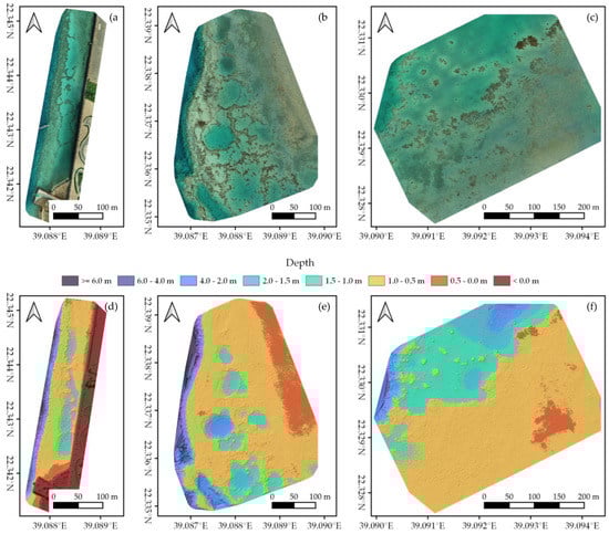
Figure 2.
Structure-from-Motion outputs of (a,d) Area 1, (b,e) Area 2, and (c,f) Area 3 (Figure 1). (a–c) The generated orthomosaics; (d–f) the corresponding Digital Elevation Models, displayed as orthometric depth.
3.2. Habitat Maps
In each survey area, we created habitat maps of the reef shallows following the four classification protocols as detailed in Section 2.7 (Figure 3, Figure 4 and Figure 5). In total, we classified an area of ~238,000 m2. We observed distinct patterns in the distribution of habitats. Namely, in all three areas, coral framework is more abundant on the reef slope and reef crest than on the reef flats, growing rarer with increasing distance to deep/open water (Figure 1, Figure 3, Figure 4 and Figure 5). At a smaller scale, underwater imagery showed a coincidal decrease in the abundance of live coral with increasing distance to the reef slope; underwater orthomosaics are available at https://doi.org/10.5061/dryad.6m905qg2p (Dataset 2). Macroalgae, sand, and seagrass show the opposite pattern and are more abundant landwards (Figure 1, Figure 3, Figure 4 and Figure 5). These patterns cannot only be observed within our survey areas but also between our survey areas at the lagoon scale (Figure 1, Figure 3, Figure 4, Figure 5, and Figure A1). The exposed Area 1 is covered for a large part by coral framework and has extensive rubble/coral pavement habitat, while macroalgae are very rare (Figure 3 and Figure A1). Area 2 is situated inside the lagoon along the main channel and contains a smaller proportion of coral framework and rubble/coral pavement habitat, while sand and macroalgae habitat become more common (Figure 1, Figure 4 and Figure A1). Area 3 is the most sheltered area surveyed. It contains very little coral framework and has a much higher presence of macroalgae and sand (Figure 5 and Figure A1). Moreover, we observed ~14,000 m2 seagrass in Area 2 and ~9000 m2 in Area 3, while seagrass was absent from Area 1 (Figure 3, Figure 4, Figure 5 and Figure A1).
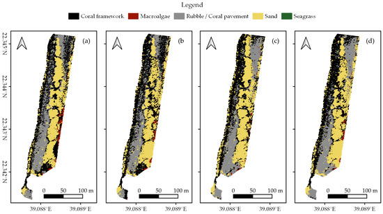
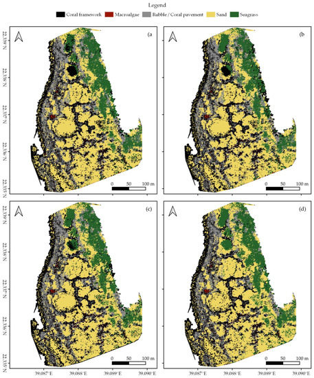
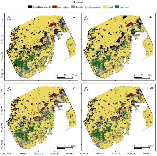
At first glance, all four classification protocols provided consistent results, displaying broadly similar habitat distributions (Figure 2, Figure 3, Figure 4, Figure 5 and Figure A1). Nonetheless, distinct differences can be observed in all three study areas. For example, the northwest corner of study Area 1 is mostly classified as rubble/coral pavement by classifiers trained on both geomorphometric and spectral features (Figure 3a,b and Figure A1). Classifiers that are only trained on spectral features, however, interpret larger areas as coral framework (Figure 3c,d and Figure A1). A similar pattern can be observed in Area 3, albeit less pronounced due to the dominance of sand habitat in this area (Figure 5 and Figure A1). In Area 2, the most notable difference between the classification protocols is how they classify a rather dark patch of seagrass at ~ 22.338° N, 39.088° E (Figure 2 and Figure 4). The less geomorphometric information the classifier has, the larger the area misclassified as coral framework (Figure 4, Dataset 1 and 3). The same type of misclassification can be observed on a smaller scale along the eastern edge of Area 2 and in the southwest corner of Area 3 (Figure 4 and Figure 5). At the scale of individual image objects, many differences can be observed scattered across all three survey areas. These differences can be inspected at full resolution in reference to the orthomosaic at https://doi.org/10.5061/dryad.6m905qg2p (Dataset 1 and 3).
3.3. Habitat Classification Accuracy
Habitat classification accuracy ranged from 0.697 for classification protocol 1. ‘Traditional classification’ in Area 1 to 0.844 for protocol 4. ‘Reef zones and geomorphometric features’ in Area 3. Except for protocol 1. ‘Traditional classification’ in Area 1, all classification protocols achieved Kappa indices between 0.6 and 0.8, indicating a ‘good’ classification accuracy (Figure 6) [78,79]. Visual observations confirmed that all classification protocols generally managed to extract the correct spatial distributions of the five habitat classes (Figure 2, Figure 3, Figure 4 and Figure 5, Dataset 1 and 3).
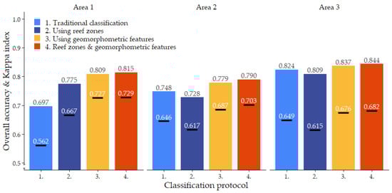
In line with the visual differences observed between the four classification protocols, there are pronounced differences in the accuracy they achieve. In all three study areas, protocol 4. ‘Reef zones and geomorphometric features’ showed the strongest performance, with an average overall accuracy of 0.816 and Kappa index of 0.705. Protocol 3. ‘Using geomorphometric features’ consistently followed as a close second, with an average overall accuracy of 0.808 and a Kappa index of 0.696. In both cases, the overall accuracy was 5% higher than the average accuracy achieved by the corresponding classification protocol that did not use geomorphometric image object features. Thus, the addition of geomorphometric features in the Random Forest algorithm increased overall accuracy by 5%. The largest increase caused by the addition of geomorphometric features to the Random Forest classifier was observed in Area 1, where the ‘Using geomorphometric features’ protocol achieved an accuracy 11.2% higher than the ‘Traditional classification’ protocol (Figure 6).
The effect of subdividing the classification over the geomorphological zones was more equivocal. For algorithms that only used spectral features during classification, subdividing the classification generated an accuracy increase of 8% in Area 1, but in Areas 2 and 3, it decreased accuracy by 2% and 1.6%, respectively. However, when the algorithm was trained on both spectral and geomorphometric features, subdividing the classification by geomorphological zone increased accuracy by a small but consistent amount of 0.6–1.1%. The combined effect of training the Random Forest algorithm on both spectral and geomorphometric features and subdividing the classification by geomorphological reef zone therefore increased accuracy by 6% on average and up to 11.8% in Area 1 (Figure 6).
Cohen’s Kappa indices mirrored the patterns described above for overall accuracy, slightly magnifying the differences between classification protocols (Figure 6).
Predictably, not every habitat class was mapped with the same accuracy. Sand habitat was classified with the highest accuracy with average producer and user accuracy of 87% and 90%, respectively. Rubble/coral pavement achieved the lowest producer and user accuracies, averaging at 63% and 40%, respectively. Coral framework was mapped with an average producer accuracy of 74% and user accuracy of 80%. For macroalgae, on average, a producer accuracy of 63% was achieved and a user accuracy of 68%. Lastly, seagrass was mapped with average producer and user accuracy of 74% and 67%, respectively (Figure 7).
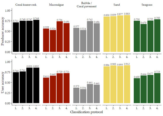
Figure 7.
Average producer and user accuracies of the four classification protocols. Classification protocols are indicated by their number (Table 2): 1. ‘Traditional classification’, 2. ‘Using reef zones’; 3. ‘Using geomorphometric features’; 4. ‘Reef zones and geomorphometric features’. For area-specific data, see (Supplementary Material Figures S6 and S7).
More importantly, incorporating geomorphometric information into the classification protocol also had a different effect in each of the five habitat classes. For example, the producer accuracy of the macroalgae and rubble/coral pavement habitat classes increased by 17% and 16%, respectively, when geomorphometric variables were incorporated into the Random Forest classifier. In contrast, the producer accuracies of the coral framework and sand habitat classes increased by 5.6% at most as a result of both the incorporation of geomorphometric variables into the Random Forest classifier and subdividing the classification over the geomorphological reef zones (Figure 7).
As for the user accuracies, using geomorphometric information impacted the coral framework, macroalgae, rubble/coral pavement, and seagrass habitat classes the most. Areas classified as coral framework, macroalgae, rubble/coral pavement, or seagrass indeed represent the correct habitat class more often when geomorphometric information was used during classification. For the coral framework and rubble/coral pavement classes, this impact is almost solely caused by the incorporation of geomorphometric variables into the Random Forest classifier. For the macroalgae and seagrass classes, a positive effect of subdividing the classification by geomorphological zone can also be observed (Figure 7).
No evident patterns were observed in the type of misclassification that was reduced by incorporating the DEM into our classification protocols. Instead, misclassifications in all alternative habitat classes were reduced by a small amount (Supplementary Material Tables S4–S15). Manual annotations used for this accuracy assessment can be compared to the orthomosaic at https://doi.org/10.5061/dryad.6m905qg2p (Dataset 1 and 3).
4. Discussion
In recent years, UAVs have revolutionised the ability to record the spatial distribution of benthic assemblages in very shallow reef habitats, but the conversion of high-resolution marine UAV imagery into accurate habitat maps is still in its infancy [22,23,24,26,28,29,41]. Here, we presented a new habitat mapping approach that incorporates not only the spectral (the orthomosaic) but also the geomorphometric (the DEM and its derivatives) output of SfM-processed UAV imagery into OBIA. Specifically, we demonstrated the possibility to: (1) semantically delineate geomorphological reef zones using the DEM, (2) then use these geomorphological zones to subdivide the habitat classification as an indirect correction for depth-related light attenuation, and (3) use DEM-derived geomorphometric variables alongside spectral features to train a Random Forest classifier. We contrasted these approaches to current methods that only make use of orthomosaic-derived spectral information [22,40,41]. The addition of geomorphometric features into the Random Forest classifier increased the accuracy of automatic habitat classification on average by 5% and up to 11%. An additional accuracy increase of 1% was achieved by performing the classification separately in each geomorphological reef zone. Thus, our methods increased overall accuracy by 6% in comparison to current methods. Crucially, our approach is easily adoptable, as most UAV-based studies already produce the necessary DEM during SfM processing [22,26,27,29,40,41,48,56,59].
By using a PPK-ready Phantom 4 Pro RTK, we were able to map ~300,000 m2 of shallow marine habitat down to 3.5 m deep. While this represents one of the most extensive marine UAV mapping efforts at this spatial resolution to date [22,24,29,40,48], it also highlights two of the main limitations faced by UAV-based monitoring of the marine environment. Firstly, even though the 300,000 m2 area we mapped here far exceeds the area that can be surveyed through scuba diving or snorkelling, it is still nowhere near the amount of area that can be surveyed with airborne or satellite imagery [15,18]. The flight time of quadcopter UAVs is strongly limited by the capacity of their batteries; hence, it is unlikely they will be able to operate at similar spatial scales to satellites or planes anytime soon. Although UAV mapping does not provide a satisfactory solution for large-scale monitoring of complete reef systems, UAVs are able to operate at much higher spatial resolutions than satellites and for a fraction of the costs of manned aircrafts, making them an efficient monitoring tool at medium scales [15,17,18,21]. We therefore argue that UAV monitoring is especially useful to monitor the effect of local stressors on coral reefs, such as polluted river outflows or coastal development. Secondly, since we rely on passive visible spectrum remote sensing, the absorption of light by the water column and the particles suspended therein limit the applicability of these methods to very shallow waters. The exact maximum operable depth must be determined on a case-by-case basis, because water clarity can vary enormously from location to location. Nonetheless, even in extremely clear water, light absorption by the water column itself will reduce the spectral distinctiveness of the different benthic components as the water becomes deeper [17,18,19,20]. Thus, the methods presented here are unlikely to produce adequate results beyond a depth of approximately six metres [20]. Because of this depth limitation, UAVs are effective tool to map reef flats, the reef crest, and the upper part of the reef slope, but a less effective tool to map the deeper areas of a coral reef. The strengths and weaknesses of UAV mapping are exactly opposite to those of acoustic mapping techniques; hence, if continuous habitat maps are required, combining these techniques may be an especially powerful approach [80].
Through OBIA, ~238,000 m2 of the total survey area was classified into five distinct benthic assemblages. Implementing our new workflow, which incorporates both UAV-derived geomorphometric and spectral information, an overall accuracy of 0.82 and a Kappa index of 0.70 were achieved, indicating a ‘good’ habitat classification [78,79]. The obtained accuracies fall in the same general range as obtained by previously published studies creating habitat maps of coral reefs based on UAV imagery. Our overall accuracy was 3% higher than attained by a comparable study in the Maldives, which classified UAV imagery of very shallow reefs with OBIA into three habitat classes: ‘hard coral’, ‘coral rubble’, and ‘sand’ [22]. At Heron Reef in Australia, Bennet et al. [23] achieved a slightly higher overall accuracy of 86% and also managed to separate live coral from dead substrate by classifying individual UAV images with a Random Forest algorithm into three habitat classes: ‘coral’, ‘rock/dead coral’, and ‘sand’. However, in this pixel-based study, the training and validation data were extracted from the same polygons, thereby limiting their spatial separation, which may have inflated the obtained accuracy [23]. Due to differences in the classified habitat classes, the study area, and the overall workflow, none of these results are directly comparable. Nevertheless, they provide a benchmark indicating that our methods indeed present a competitive alternative to currently available methodologies.
Integrating geomorphometric variables into the Random Forest algorithm consistently increased overall accuracy, with increases of up to 11.2% being observed (Figure 6). Therefore, the UAV-derived DEM and derivatives thereof clearly contain habitat-differentiating information and can be used to increase the accuracy of automatic habitat classification. Not every habitat class was affected equally by the addition of geomorphometric information into the classification protocol. Classification accuracies of macroalgae and rubble/coral pavement habitats were affected the most and those of the sand class the least (Figure 7), which is one of the reasons why the magnitude of the accuracy increase achieved by our new methods differs substantially among the three survey areas. In Area 1, the rubble/coral pavement habitat class, which shows stark accuracy increases, is relatively abundant. This likely contributed to the large increase in overall accuracy observed there (Figure 3, Figure 6 and Figure 7). In contrast, in Area 3, where the sand habitat class is dominant, a much smaller increase in accuracy was observed (Figure 5, Figure 6 and Figure 7). We note that our new workflow increased classification accuracy especially in those habitats that proved the most challenging for traditional ‘spectral’ workflows (Figure 7). While these habitat classes naturally left the most room for improvement, this result also highlights the complementary nature of the UAV’s DEM compared to the orthomosaic. We therefore expect that, in combination with a Random Forest classifier that is able to prioritise the most useful data for each specific split in the data [77], our methods are likely to provide accuracy increases in many different scenarios also outside of coral reef mapping [42,43,44,46].
A potential caveat of using an SfM-derived DEM in habitat classification of the marine environment is the presence of SfM processing errors in the DEM. Depending on the local conditions—with respect to shade, bottom texture, waves, water depth, and glint—SfM algorithms can struggle to correctly reconstruct bathymetry (Dataset 1) [25]. While such distortions are minimised by careful flight planning, the inclusion of PPK into our SfM workflow, manual cleaning of the dense point cloud, and filtering the DEM, they are never fully removed. Therefore, distortions may persist, especially along the edges of the survey area and in deeper areas with little bottom structure (Dataset 1). This could affect classification procedures. However, in this study, the addition of geomorphometric variables into the Random Forest classification algorithm still improved habitat classification accuracies in every single classification (Figure 6 and Figure 7). In fact, the highest accuracy increase was observed in Area 1, where SfM distortions were the most pronounced due to slightly windier conditions during image acquisition (Figure 1, Figure 6 and Figure 7 and Dataset 1). We identify two important reasons why our automatic habitat classifications did not suffer from the remaining distortions in the DEM. Firstly, Random Forest algorithms are known to be particularly robust to noise in their input data [43,45,46,77]. Secondly, SfM processing errors are partially dependent on the texture visible in the images. If an image area has more texture, it is easier for the feature detection algorithms of SfM to recognise specific points among multiple images [31,81]. This means that SfM processing errors can be influenced by the local habitat class because they provide texture to the UAV images. Thus, the SfM processing errors may at least in part be consistent with the underlying habitat class. If this were the case, it would allow the Random Forest classifier to identify processing errors as a unique habitat feature. Persistent errors may therefore assist in correct habitat classification instead of hampering it.
The fact that SfM-derived geomorphometric variables can provide habitat-differentiating data even in challenging marine environments is important because other methods that can acquire similar data, such as airborne LiDAR or multi-spectral imagery, require more expensive, specialised equipment [15,25,82]. We realise that although the Phantom 4 RTK provides a relatively cheap alternative to such techniques and even other RTK-ready UAVS, its price of USD 6450 still far exceeds that of regular consumer-grade UAVs. A full overview of the start-up costs of this research is available in the Supplementary Materials Section S6. It would therefore be interesting to see whether DEMs created with consumer-grade UAVs without RTK capabilities can also be used to improve automatic habitat classification. Because such UAVs are more widely distributed and significantly cheaper than RTK-ready UAVs, this would make our methods much more accessible. Since the Random Forest classifier seems to be relatively robust with respect to noise in the DEM, we argue that in good weather conditions and with the incorporation of extra GCPs, this should be possible.
Besides increasing habitat classification accuracy, the UAV-derived DEM also allowed for the semantic subdivision of the reef’s geomorphological zones in OBIA. In this study, the reef’s geomorphological zones were delineated using depth directly, but other possibilities exist. For example, the reef slope could also have been identified with a DEM-derived, low-resolution slope raster. Regardless of the specific implementation, this method provided a well-documented, semantic decision process on the delineation of the geomorphological reef zones. This provides a clear advantage over manual or spectral rule-based delineations as it is easier to understand and it simplifies inter-study comparisons [47,83]. In addition, using the DEM provided a much quicker workflow than manual annotation. However, in contrast to habitat classification with Random Forest algorithms, the delineation of reef areas directly based on depth or other geomorphometric thresholds is susceptible to SfM processing errors. For instance, in Area 2 at ~22.3365° N, 39.0868° E, a triangular area is classified as coral framework, but it should have been excluded from the analysis as part of the ‘deep water’ zone (Figure 2 and Figure 4). Because SfM processing errors are easily identifiable in the DEM (Dataset 1) such misclassifications can be avoided through manual editing. Here, we refrained from any manual editing of the DEM to be able to highlight both the strengths and weaknesses of our approach.
In this study, subdividing the classification by the aforementioned geomorphological reef zones did not consistently improve mapping accuracy by indirectly correcting for depth-related effects of light attenuation, as suggested by Monteiro et al. [48]. When the algorithm was trained solely on spectral image features, subdividing the classification increased accuracy only in one out of three cases (Figure 6). When the Random Forest algorithm was trained on both spectral and geomorphometric features, accuracy increased consistently by about 1% (Figure 6). Besides the limited depth-range surveyed here, we attribute this effect to the fact that subdividing the classification also severely limited the number of samples available to each separate Random Forest algorithm during classification. Small sample sizes restrict the independence of the individual trees the Random Forest algorithm creates, reducing the algorithm’s accuracy. This effect is more pronounced if the amount of classification features is also limited, as both randomly sampling the classification features and samples is used to create independence among individual trees in Random Forest algorithms [77]. Thus, subdividing the classification restricts tree independence more strongly in our protocols that only use spectral image features, seemingly causing a less stable performance of our Random Forest algorithm. To circumvent this issue, future studies are encouraged to explore the possibilities to directly, mathematically correct the effects of light attenuation—for instance, through an adaptation of the methods presented by Conger et al. [49].
The habitat maps presented here are some of the first to characterise our study area in very high spatial resolution. While the broad classification scheme used in this study cannot represent the full heterogeneity of the ecosystem, our habitat maps did reveal spatial patterns within the ecosystem that otherwise may have gone unnoticed. Thus, some new insights in the ecosystem’s structure and functioning were obtained [10,14]. For example, the abundance of reef framework that is overgrown by macroalgae in Area 3 could be the result of a shift in ecosystem functioning inside the lagoon from a coral-dominated to a macroalgae-dominated state that is not yet observed at the lagoon’s entrance in Area 1 (Figure 1, Figure 3 and Figure 5) [1,7,8,84]. This is corroborated by our underwater imagery, which shows a sharp decline in live coral cover with increasing distance to the reef slope and deep water habitat, where live coral is still abundant (Dataset 3). The reef flats inside this lagoon therefore currently seem to support a limited community of live corals. As these reef flats represent the shallowest and most landward habitat occupied by corals, it is possible that the natural conditions in this very shallow environment are becoming too extreme for them to strive. Alternatively, we suspect that the global coral bleaching events of 2010 and 2015/2016 might have been highly detrimental to former populations occupying these areas [3,4,5]. Since then, coral recovery has apparently been limited on these shallow reef flats. Despite the low occurrence of live coral, the lagoon’s reef flats at the study site still fulfil important ecological functions. For example, the ~38,000 m2 of coral framework we identified was clearly preferred over the other habitats by herbivorous reef fish (personal observation, B.O.N.) (Figure A1), likely as a result of the refuge possibilities and the abundance of palatable algae that the coral framework offers (Dataset 3) [33,85]. On the other hand, three genera of stingray, Taeniuara, Pastinachus, and Himantura, were frequently observed on the sand flats (personal observation, B.O.N.) [86]. Ubiquitous ray pits indicated that rays likely feed on the benthic infauna of these sand flats (Dataset 1) [87,88,89]. Moreover, we identified ~23.000 m2 of seagrass habitat, which is an important nursery habitat for coral reef fish and decapods [90,91] that can support increased numbers of benthic infauna [92]. Because all our habitat classes represent different communities that fulfil different ecological functions, understanding their spatial distribution is highly relevant to their conservation. The high spatial resolution habitat maps we have presented here therefore provide new information on the ecological functioning of the lagoon that could support ecosystem-based management decision making [9,10,12]. Additionally, our habitat maps provide baseline measurements that can be used for future change detection studies [22,83].
We argue that the potential of the UAV-derived DEM for marine habitat mapping is not dependent on the specifics of this study but is more widely applicable. We therefore highly encourage future studies to not only apply but also elaborate on these methods. For instance, in this study, we used a Random Forest algorithm to perform automatic habitat classification, but many efficient classification algorithms exist that may also benefit from the incorporation of geomorphometric parameters. Within eCognition, alternatives include Bayes, k-Nearest Neighbour, Support Vector Machine, Decision Tree, and Convolutional Neural Network classification algorithms. The implementation of the described methods into modern deep learning classifiers such as Convolutional Neural Networks is of particular interest, because—if given sufficient training data—such algorithms may substantially outperform traditional classifiers such as Random Forest or Support Vector Machines [93]. Ultimately, this may lead to classification models that are also able to correctly classify spatially separated datasets. Furthermore, the geomorphometric features used in this study do not constitute an exhaustive list. Rather, they represent a subset of commonly used geomorphometric parameters that were expected to be useful in habitat identification [43,45,69,70,71,72]. We therefore highly encourage future studies to experiment with additional DEM-derived geomorphometric variables. Ideally, such investigations include an extensive optimisation/feature selection process so a selection of the most useful geomorphometric variables can be established. This becomes particularly important if a different classification algorithm is used (other than a Random Forest algorithm). While the Random Forest algorithm has the inherent ability to internally prioritise the most important classification features, other algorithms may be more sensitive to the inclusion of non-informative features [45,77], as we encountered during initial trials with the k-Nearest Neighbour algorithm. If easy implementation is required—for example, in management scenarios—we advise sticking to a Random Forest classifier, for which extensive knowledge on the habitat-differentiating qualities of individual geomorphometric variables is not needed [36]. Another promising future direction is the incorporation of the DEM and its derivatives in the segmentation step of OBIA. The segmentation accuracy can have a profound impact on the accuracy of the eventual classification in OBIA [75]. Under-segmentation, where multiple habitat classes are grouped together into a single image object, directly limits the maximum attainable accuracy. In contrast, over-segmentation does not necessarily limit accuracy, but it does limit the advantages of using OBIA over pixel-based methods [75]. DEMs and their derived geomorphometric variables can possibly also assist the segmentation algorithm in correctly identifying boundaries between different habitat types, further increasing the final classification accuracy. Finally, the OBIA framework and Random Forest classifiers are well suited to handle a large collection of independent input data, as is evident in this study, where we combined multiple DEM-derived rasters with an orthomosaic. Recent studies have successfully used UAV-derived multispectral images for marine habitat mapping [24,26,27,94]. Besides providing spectral information of a higher spectral resolution, multi-spectral imagery also provides alternative methods to accurately retrieve bathymetry [49,50,82,94]. The automatic classification of multi-spectral UAV imagery in combination with UAV-derived geomorphometric rasters in an OBIA framework thus seems promising.
5. Conclusions
We have demonstrated a new workflow for habitat mapping of shallow marine ecosystems in OBIA that integrates not only the orthomosaic generated by SfM-processed UAV imagery, but also the DEM. Benefitting from the habitat-differentiating information contained within the SfM-derived DEM, we were able to increase the overall accuracy of automatic habitat classification by 6% on average without requiring any additional sampling effort. Ultimately, the production of more accurate habitat maps can assist in ecosystem-based management decision making, which is crucial for the continued survival of shallow coral reefs in the Anthropocene.
Supplementary Materials
The following supporting information can be downloaded at: https://www.mdpi.com/article/10.3390/rs14195017/s1, Figure S1: GoPro camera array used during snorkel transects; Figure S2: DEM generation in Pix4Dmapper using (a) the Inverse Distance Weighting method or (b) the Triangulation method; Figures S3–S5: Correlation matrices of the geomorphometric variables per Area; Figure S6: Producer accuracies of the four classification protocols, subdivided per survey area; Figure S7: User accuracies of the four classification protocols, subdivided per survey area; Table S1: GoPro settings used during snorkel transects; Table S2: SfM processing settings used to process UAV imagery in Pix4Dmapper; Table S3: SfM processing settings used to process underwater imagery in Agisoft Metashape; Tables S4–S7: Contingency tables—Area 1; Tables S8–S11: Contingency table—Area 2; Tables S12–S15: Contingency tables—Area 3. References [31,56,58,59,63,64,65] are cited in the Supplementary Materials.
Author Contributions
Conceptualisation, B.O.N. and F.M.; data acquisition, B.O.N., M.C., and A.S.; methodology, B.O.N., F.M., M.C., and A.S.; formal analysis, B.O.N.; funding acquisition F.B.; supervision F.M., F.B., and S.E.T.V.d.M.; visualisation, B.O.N.; writing—original draft preparation, B.O.N.; writing—review and editing, B.O.N., F.M., S.E.T.V.d.M., and F.B. All authors have read and agreed to the published version of the manuscript.
Funding
This research was funded by KAUST and baseline research funds to F.B. (BAS11090-01-01). This research was partially supported by the Groningen University Fund with an Outstanding Master Student grant, awarded to B.O.N. (2021AU050).
Institutional Review Board Statement
Not applicable.
Data Availability Statement
The data presented in this study are available online in the DRYAD repository at: https://doi.org/10.5061/dryad.6m905qg2p. The following materials can be downloaded: Dataset 1: UAV orthomosaics and DEMs; Dataset 2: Snorkel transect orthomosaics; Dataset 3: Habitat classifications; Dataset 4: Manual classifications for accuracy assessment.
Acknowledgments
We would like to thank members of the Habitat and Benthic Biodiversity lab for their assistance in the field, notably Laura Macrina, Aymere Assayie, Federica Barreca, Francesca Giovenzana, and Silvia Vicario. We also extend our thanks to Colleen Campbell and Ioana Andreea Ciocanaru for lending us the UAV Ground Control Points. Finally, we would like to thank the reviewers for providing knowledgeable comments on an earlier version of this manuscript.
Conflicts of Interest
The authors declare no conflict of interest. The funders had no role in the design of the study; in the collection, analyses, or interpretation of data; in the writing of the manuscript, or in the decision to publish the results.
Appendix A

Figure A1.
Surface area of each habitat as classified in eCognition separated by survey area and classification protocol (Figure 1, and Table 2). Classification protocols are indicated by their number (Table 2): 1. ‘Traditional classification’, 2. ‘Using reef zones’; 3. ‘Using geomorphometric features’; 4. ‘Reef zones and geomorphometric features’.

References
- Bellwood, D.R.; Hughes, T.P.; Folke, C.; Nyström, M. Confronting the coral reef crisis. Nature 2004, 429, 827–833. [Google Scholar] [CrossRef] [PubMed]
- Hughes, T.P.; Kerry, J.T.; Álvarez-Noriega, M.; Álvarez-Romero, J.G.; Anderson, K.D.; Baird, A.H.; Babcock, R.C.; Beger, M.; Bellwood, D.R.; Berkelmans, R.; et al. Global warming and recurrent mass bleaching of corals. Nature 2017, 543, 373–377. [Google Scholar] [CrossRef] [PubMed]
- Baird, A.; Madin, J.; Álvarez-Noriega, M.; Fontoura, L.; Kerry, J.; Kuo, C.; Precoda, K.; Torres-Pulliza, D.; Woods, R.; Zawada, K.; et al. A decline in bleaching suggests that depth can provide a refuge from global warming in most coral taxa. Mar. Ecol. Prog. Ser. 2018, 603, 257–264. [Google Scholar] [CrossRef]
- Monroe, A.A.; Ziegler, M.; Roik, A.; Röthig, T.; Hardenstine, R.S.; Emms, M.A.; Jensen, T.; Voolstra, C.R.; Berumen, M.L. In situ observations of coral bleaching in the central Saudi Arabian Red Sea during the 2015/2016 global coral bleaching event. PLoS ONE 2018, 13, e0195814. [Google Scholar] [CrossRef] [PubMed]
- Furby, K.A.; Bouwmeester, J.; Berumen, M.L. Susceptibility of central Red Sea corals during a major bleaching event. Coral Reefs 2013, 32, 505–513. [Google Scholar] [CrossRef]
- Mumby, P.J.; Steneck, R.S. Coral reef management and conservation in light of rapidly evolving ecological paradigms. Trends Ecol. Evol. 2008, 23, 555–563. [Google Scholar] [CrossRef] [PubMed]
- Brandl, S.J.; Rasher, D.B.; Côté, I.M.; Casey, J.M.; Darling, E.S.; Lefcheck, J.S.; Duffy, J.E. Coral reef ecosystem functioning: Eight core processes and the role of biodiversity. Front. Ecol. Environ. 2019, 17, 445–454. [Google Scholar] [CrossRef]
- Hughes, T.P.; Barnes, M.L.; Bellwood, D.R.; Cinner, J.E.; Cumming, G.S.; Jackson, J.B.C.; Kleypas, J.; van de Leemput, I.A.; Lough, J.M.; Morrison, T.H.; et al. Coral reefs in the Anthropocene. Nature 2017, 546, 82–90. [Google Scholar] [CrossRef] [PubMed]
- McLeod, K.L.; Lubchenco, J.; Palumbi, S.; Rosenberg, A.A. Scientific Consensus Statement on Marine Ecosystem-Based Management. 2005, 1–5. Available online: https://marineplanning.org/wp-content/uploads/2015/07/Consensusstatement.pdf (accessed on 27 June 2022).
- Crowder, L.; Norse, E. Essential ecological insights for marine ecosystem-based management and marine spatial planning. Mar. Policy 2008, 32, 772–778. [Google Scholar] [CrossRef]
- Ehler, C.; Douvere, F. Marine Spatial Planning: A Step-by-Step Approach. IOC. Available online: https://www.oceanbestpractices.net/handle/11329/459 (accessed on 27 June 2022).
- Cogan, C.B.; Todd, B.J.; Lawton, P.; Noji, T.T. The role of marine habitat mapping in ecosystem-based management. ICES J. Mar. Sci. 2009, 66, 2033–2042. [Google Scholar] [CrossRef]
- Baker, E.K.; Harris, P.T. Habitat mapping and marine management. In Seafloor Geomorphology as Benthic Habitat; Elsevier: Amsterdam, The Netherlands, 2020; pp. 17–33. ISBN 9780128149607. [Google Scholar]
- Harris, P.T.; Baker, E.K. Why map benthic habitats? In Seafloor Geomorphology as Benthic Habitat; Elsevier: Amsterdam, The Netherlands, 2020; pp. 3–15. ISBN 9780128149607. [Google Scholar]
- Hamylton, S.M. Mapping coral reef environments. Prog. Phys. Geogr. Earth Environ. 2017, 41, 803–833. [Google Scholar] [CrossRef]
- Costa, B.M.; Battista, T.A.; Pittman, S.J. Comparative evaluation of airborne LiDAR and ship-based multibeam SoNAR bathymetry and intensity for mapping coral reef ecosystems. Remote Sens. Environ. 2009, 113, 1082–1100. [Google Scholar] [CrossRef]
- Purkis, S.J. Remote Sensing Tropical Coral Reefs: The View from Above. Ann. Rev. Mar. Sci. 2018, 10, 149–168. [Google Scholar] [CrossRef] [PubMed]
- Joyce, K.E.; Duce, S.; Leahy, S.M.; Leon, J.; Maier, S.W. Principles and practice of acquiring drone-based image data in marine environments. Mar. Freshw. Res. 2019, 70, 952. [Google Scholar] [CrossRef]
- Roelfsema, C.; Phinn, S.R. Integrating field data with high spatial resolution multispectral satellite imagery for calibration and validation of coral reef benthic community maps. J. Appl. Remote Sens. 2010, 4, 043527. [Google Scholar] [CrossRef]
- Leiper, I.A.; Phinn, S.R.; Roelfsema, C.M.; Joyce, K.E.; Dekker, A.G. Mapping Coral Reef Benthos, Substrates, and Bathymetry, Using Compact Airborne Spectrographic Imager (CASI) Data. Remote Sens. 2014, 6, 6423–6445. [Google Scholar] [CrossRef]
- Anderson, K.; Gaston, K.J. Lightweight unmanned aerial vehicles will revolutionize spatial ecology. Front. Ecol. Environ. 2013, 11, 138–146. [Google Scholar] [CrossRef]
- Fallati, L.; Saponari, L.; Savini, A.; Marchese, F.; Corselli, C.; Galli, P. Multi-Temporal UAV Data and Object-Based Image Analysis (OBIA) for Estimation of Substrate Changes in a Post-Bleaching Scenario on a Maldivian Reef. Remote Sens. 2020, 12, 2093. [Google Scholar] [CrossRef]
- Bennett, M.K.; Younes, N.; Joyce, K. Automating Drone Image Processing to Map Coral Reef Substrates Using Google Earth Engine. Drones 2020, 4, 50. [Google Scholar] [CrossRef]
- Cornet, V.J.; Joyce, K.E. Assessing the Potential of Remotely-Sensed Drone Spectroscopy to Determine Live Coral Cover on Heron Reef. Drones 2021, 5, 29. [Google Scholar] [CrossRef]
- David, C.G.; Kohl, N.; Casella, E.; Rovere, A.; Ballesteros, P.; Schlurmann, T. Structure-from-Motion on shallow reefs and beaches: Potential and limitations of consumer-grade drones to reconstruct topography and bathymetry. Coral Reefs 2021, 40, 835–851. [Google Scholar] [CrossRef]
- Mohamad, M.N.; Reba, M.N.; Hossain, M.S. A screening approach for the correction of distortion in UAV data for coral community mapping. Geocarto Int. 2021, 37, 7089–7121. [Google Scholar] [CrossRef]
- Muslim, A.M.; Chong, W.S.; Safuan, C.D.M.; Khalil, I.; Hossain, M.S. Coral Reef Mapping of UAV: A Comparison of Sun Glint Correction Methods. Remote Sens. 2019, 11, 2422. [Google Scholar] [CrossRef]
- Collin, A.; Ramambason, C.; Pastol, Y.; Casella, E.; Rovere, A.; Thiault, L.; Espiau, B.; Siu, G.; Lerouvreur, F.; Nakamura, N.; et al. Very high resolution mapping of coral reef state using airborne bathymetric LiDAR surface-intensity and drone imagery. Int. J. Remote Sens. 2018, 39, 5676–5688. [Google Scholar] [CrossRef]
- Casella, E.; Collin, A.; Harris, D.; Ferse, S.; Bejarano, S.; Parravicini, V.; Hench, J.L.; Rovere, A. Mapping coral reefs using consumer-grade drones and structure from motion photogrammetry techniques. Coral Reefs 2017, 36, 269–275. [Google Scholar] [CrossRef]
- Chirayath, V.; Earle, S.A. Drones that see through waves—Preliminary results from airborne fluid lensing for centimetre-scale aquatic conservation. Aquat. Conserv. Mar. Freshw. Ecosyst. 2016, 26, 237–250. [Google Scholar] [CrossRef]
- Westoby, M.J.; Brasington, J.; Glasser, N.F.; Hambrey, M.J.; Reynolds, J.M. ‘Structure-from-Motion’ photogrammetry: A low-cost, effective tool for geoscience applications. Geomorphology 2012, 179, 300–314. [Google Scholar] [CrossRef]
- Burns, J.H.R.; Delparte, D.; Gates, R.D.; Takabayashi, M. Integrating structure-from-motion photogrammetry with geospatial software as a novel technique for quantifying 3D ecological characteristics of coral reefs. PeerJ 2015, 3, e1077. [Google Scholar] [CrossRef]
- Graham, N.A.J.; Nash, K.L. The importance of structural complexity in coral reef ecosystems. Coral Reefs 2013, 32, 315–326. [Google Scholar] [CrossRef]
- Miller, S.; Yadav, S.; Madin, J.S. The contribution of corals to reef structural complexity in Kāne‘ohe Bay. Coral Reefs 2021, 40, 1679–1685. [Google Scholar] [CrossRef]
- Carlot, J.; Rovère, A.; Casella, E.; Harris, D.; Grellet-Muñoz, C.; Chancerelle, Y.; Dormy, E.; Hedouin, L.; Parravicini, V. Community composition predicts photogrammetry-based structural complexity on coral reefs. Coral Reefs 2020, 39, 967–975. [Google Scholar] [CrossRef]
- Andréfouët, S. Coral reef habitat mapping using remote sensing: A user vs. producer perspective. implications for research, management and capacity building. J. Spat. Sci. 2008, 53, 113–129. [Google Scholar] [CrossRef]
- Blaschke, T. Object based image analysis for remote sensing. ISPRS J. Photogramm. Remote Sens. 2010, 65, 2–16. [Google Scholar] [CrossRef]
- Blaschke, T.; Hay, G.J.; Kelly, M.; Lang, S.; Hofmann, P.; Addink, E.; Feitosa, R.Q.; van der Meer, F.; van der Werff, H.; van Coillie, F.; et al. Geographic Object-Based Image Analysis—Towards a new paradigm. ISPRS J. Photogramm. Remote Sens. 2014, 87, 180–191. [Google Scholar] [CrossRef]
- Benz, U.C.; Hofmann, P.; Willhauck, G.; Lingenfelder, I.; Heynen, M. Multi-resolution, object-oriented fuzzy analysis of remote sensing data for GIS-ready information. ISPRS J. Photogramm. Remote Sens. 2004, 58, 239–258. [Google Scholar] [CrossRef]
- Ventura, D.; Bonifazi, A.; Gravina, M.F.; Belluscio, A.; Ardizzone, G. Mapping and Classification of Ecologically Sensitive Marine Habitats Using Unmanned Aerial Vehicle (UAV) Imagery and Object-Based Image Analysis (OBIA). Remote Sens. 2018, 10, 1331. [Google Scholar] [CrossRef]
- Nababan, B.; Mastu, L.O.K.; Idris, N.H.; Panjaitan, J.P. Shallow-Water Benthic Habitat Mapping Using Drone with Object Based Image Analyses. Remote Sens. 2021, 13, 4452. [Google Scholar] [CrossRef]
- Sumesh, K.C.; Ninsawat, S.; Som-ard, J. Integration of RGB-based vegetation index, crop surface model and object-based image analysis approach for sugarcane yield estimation using unmanned aerial vehicle. Comput. Electron. Agric. 2021, 180, 105903. [Google Scholar] [CrossRef]
- Juel, A.; Groom, G.B.; Svenning, J.-C.; Ejrnæs, R. Spatial application of Random Forest models for fine-scale coastal vegetation classification using object based analysis of aerial orthophoto and DEM data. Int. J. Appl. Earth Obs. Geoinf. 2015, 42, 106–114. [Google Scholar] [CrossRef]
- Kraaijenbrink, P.D.A.; Shea, J.M.; Pellicciotti, F.; Jong, S.M.; de Immerzeel, W.W. Object-based analysis of unmanned aerial vehicle imagery to map and characterise surface features on a debris-covered glacier. Remote Sens. Environ. 2016, 186, 581–595. [Google Scholar] [CrossRef]
- Rodriguez-Galiano, V.F.; Ghimire, B.; Rogan, J.; Chica-Olmo, M.; Rigol-Sanchez, J.P. An assessment of the effectiveness of a random forest classifier for land-cover classification. ISPRS J. Photogramm. Remote Sens. 2012, 67, 93–104. [Google Scholar] [CrossRef]
- Lebourgeois, V.; Dupuy, S.; Vintrou, É.; Ameline, M.; Butler, S.; Bégué, A. A Combined Random Forest and OBIA Classification Scheme for Mapping Smallholder Agriculture at Different Nomenclature Levels Using Multisource Data (Simulated Sentinel-2 Time Series, VHRS and DEM). Remote Sens. 2017, 9, 259. [Google Scholar] [CrossRef]
- Phinn, S.R.; Roelfsema, C.M.; Mumby, P.J. Multi-scale, object-based image analysis for mapping geomorphic and ecological zones on coral reefs. Int. J. Remote Sens. 2012, 33, 3768–3797. [Google Scholar] [CrossRef]
- Monteiro, J.G.; Jiménez, J.L.; Gizzi, F.; Přikryl, P.; Lefcheck, J.S.; Santos, R.S.; Canning-Clode, J. Novel approach to enhance coastal habitat and biotope mapping with drone aerial imagery analysis. Sci. Rep. 2021, 11, 1–13. [Google Scholar] [CrossRef]
- Conger, C.L.; Hochberg, E.J.; Fletcher, C.H.; Atkinson, M.J. Decorrelating remote sensing color bands from bathymetry in optically shallow waters. IEEE Trans. Geosci. Remote Sens. 2006, 44, 1655–1660. [Google Scholar] [CrossRef]
- Stumpf, R.P.; Holderied, K.; Sinclair, M. Determination of water depth with high-resolution satellite imagery over variable bottom types. Limnol. Oceanogr. 2003, 48, 547–556. [Google Scholar] [CrossRef]
- Fine, M.; Cinar, M.; Voolstra, C.R.; Safa, A.; Rinkevich, B.; Laffoley, D.; Hilmi, N.; Allemand, D. Coral reefs of the Red Sea—Challenges and potential solutions. Reg. Stud. Mar. Sci. 2019, 25, 100498. [Google Scholar] [CrossRef]
- DJI. Phantom 4 RTK User Manual V2.4. Available online: https://www.dji.com/nl/downloads/products/phantom-4-rtk (accessed on 27 June 2022).
- Pugh, D.T.; Abualnaja, Y.; Jarosz, E. The Tides of the Red Sea. In Oceanographic and Biological Aspects of the Red Sea; Rasul, N.M.A., Stewart, I.C.F., Eds.; Springer Nature: Cham, Switzerland, 2019; pp. 11–40. ISBN 9783319994161. [Google Scholar]
- James, M.R.; Robson, S. Mitigating systematic error in topographic models derived from UAV and ground-based image networks. Earth Surf. Process. Landforms 2014, 39, 1413–1420. [Google Scholar] [CrossRef]
- Štroner, M.; Urban, R.; Seidl, J.; Reindl, T.; Brouček, J. Photogrammetry Using UAV-Mounted GNSS RTK: Georeferencing Strategies without GCPs. Remote Sens. 2021, 13, 1336. [Google Scholar] [CrossRef]
- Taddia, Y.; Stecchi, F.; Pellegrinelli, A. Coastal Mapping Using DJI Phantom 4 RTK in Post-Processing Kinematic Mode. Drones 2020, 4, 9. [Google Scholar] [CrossRef]
- James, M.R.; Robson, S.; D’Oleire-Oltmanns, S.; Niethammer, U. Optimising UAV topographic surveys processed with structure-from-motion: Ground control quality, quantity and bundle adjustment. Geomorphology 2017, 280, 51–66. [Google Scholar] [CrossRef]
- Przybilla, H.-J.; Bäumker, M.; Luhmann, T.; Hastedt, H.; Eilers, M. Interaction between direct georeferencing, control point configuration and camera self-calibration for RTK-based UAV photogrammetry. Int. Arch. Photogramm. Remote Sens. Spat. Inf. Sci. 2020, 43, 485–492. [Google Scholar] [CrossRef]
- Tomaštík, J.; Mokroš, M.; Surový, P.; Grznárová, A.; Merganič, J. UAV RTK/PPK Method—An Optimal Solution for Mapping Inaccessible Forested Areas? Remote Sens. 2019, 11, 721. [Google Scholar] [CrossRef]
- Famiglietti, N.A.; Cecere, G.; Grasso, C.; Memmolo, A.; Vicari, A. A Test on the Potential of a Low Cost Unmanned Aerial Vehicle RTK/PPK Solution for Precision Positioning. Sensors 2021, 21, 3882. [Google Scholar] [CrossRef]
- General Authority for Survey and Geospatial Information KSACORS. Available online: https://ksacors.gcs.gov.sa/ (accessed on 22 February 2022).
- REDcatch GmbH. REDtoolbox v2.82 User Manual. Available online: https://www.redcatch.at/downloads_all/REDtoolbox_manual_EN.pdf (accessed on 2 October 2022).
- Jiang, S.; Jiang, C.; Jiang, W. Efficient structure from motion for large-scale UAV images: A review and a comparison of SfM tools. ISPRS J. Photogramm. Remote Sens. 2020, 167, 230–251. [Google Scholar] [CrossRef]
- Sona, G.; Pinto, L.; Pagliari, D.; Passoni, D.; Gini, R. Experimental analysis of different software packages for orientation and digital surface modelling from UAV images. Earth Sci. Inf. 2014, 7, 97–107. [Google Scholar] [CrossRef]
- Burns, J.H.R.; Delparte, D. Comparison of commercial Structure-from-Motion photogrammetry software used for underwater three-dimensional modeling of Coral reef environments. Int. Arch. Photogramm. Remote Sens. Spat. Inf. Sci. 2017, XLII-2/W3, 127–131. [Google Scholar] [CrossRef]
- Conrad, O.; Bechtel, B.; Bock, M.; Dietrich, H.; Fischer, E.; Gerlitz, L.; Wehberg, J.; Wichmann, V.; Böhner, J. System for Automated Geoscientific Analyses (SAGA) v. 2.1.4. Geosci. Model Dev. 2015, 8, 1991–2007. [Google Scholar] [CrossRef]
- General Authority Geospatial Information. SANSRS Transformation Tools. Available online: https://gds.gasgi.gov.sa/ (accessed on 9 March 2022).
- General Authority Geospatial Information. Technical Summary for Saudi Arabia National Spatial Reference System (SANSRS). Available online: https://www.gasgi.gov.sa/En/Products/Geodesy/Documents/Technical Summary for SANSRS.pdf (accessed on 27 June 2022).
- Zevenbergen, L.W.; Thorne, C.R. Quantitative analysis of land surface topography. Earth Surf. Process. Landforms 1987, 12, 47–56. [Google Scholar] [CrossRef]
- Sappington, J.M.; Longshore, K.M.; Thompson, D.B. Quantifying Landscape Ruggedness for Animal Habitat Analysis: A Case Study Using Bighorn Sheep in the Mojave Desert. J. Wildl. Manag. 2007, 71, 1419–1426. [Google Scholar] [CrossRef]
- Guisan, A.; Weiss, S.B.; Weiss, A.D. GLM versus CCA Spatial Modeling of Plant Species Distribution. Plant Ecol. 1999, 143, 107–122. [Google Scholar] [CrossRef]
- Zimmermann, N.E. Toposcale.Aml. Available online: www.wsl.ch/staff/niklaus.zimmermann/programs/aml4_1.html (accessed on 9 March 2022).
- Trimble GmbH. User Guide eCognition Developer. Available online: https://docs.ecognition.com/v9.5.0/Page collection/eCognition Suite Dev UG.htm (accessed on 27 June 2022).
- Roelfsema, C.; Kovacs, E.; Roos, P.; Terzano, D.; Lyons, M.; Phinn, S. Use of a semi-automated object based analysis to map benthic composition, Heron Reef, Southern Great Barrier Reef. Remote Sens. Lett. 2018, 9, 324–333. [Google Scholar] [CrossRef]
- Liu, D.; Xia, F. Assessing object-based classification: Advantages and limitations. Remote Sens. Lett. 2010, 1, 187–194. [Google Scholar] [CrossRef]
- Drăguţ, L.; Csillik, O.; Eisank, C.; Tiede, D. Automated parameterisation for multi-scale image segmentation on multiple layers. ISPRS J. Photogramm. Remote Sens. 2014, 88, 119–127. [Google Scholar] [CrossRef] [PubMed]
- Breiman, L. Random Forests. Mach. Learn. 2001, 45, 5–32. [Google Scholar] [CrossRef]
- Landis, J.R.; Koch, G.G. The Measurement of Observer Agreement for Categorical Data. Biometrics 1977, 33, 159. [Google Scholar] [CrossRef]
- Lehmann, J.; Nieberding, F.; Prinz, T.; Knoth, C. Analysis of Unmanned Aerial System-Based CIR Images in Forestry—A New Perspective to Monitor Pest Infestation Levels. Forests 2015, 6, 594–612. [Google Scholar] [CrossRef]
- Rende, S.F.; Bosman, A.; di Mento, R.; Bruno, F.; Lagudi, A.; Irving, A.D.; Dattola, L.; Giambattista, L.; di Lanera, P.; Proietti, R.; et al. Ultra-High-Resolution Mapping of Posidonia oceanica (L.) Delile Meadows through Acoustic, Optical Data and Object-based Image Classification. J. Mar. Sci. Eng. 2020, 8, 647. [Google Scholar] [CrossRef]
- Hafeez, J.; Jeon, H.J.; Hamacher, A.; Kwon, S.C.; Lee, S.H. The effect of patterns on image-based modelling of texture-less objects. Metrol. Meas. Syst. 2018, 25, 755–767. [Google Scholar] [CrossRef]
- Rossi, L.; Mammi, I.; Pelliccia, F. UAV-Derived Multispectral Bathymetry. Remote Sens. 2020, 12, 3897. [Google Scholar] [CrossRef]
- Roelfsema, C.M.; Lyons, M.; Kovacs, E.M.; Maxwell, P.; Saunders, M.I.; Samper-Villarreal, J.; Phinn, S.R. Multi-temporal mapping of seagrass cover, species and biomass: A semi-automated object based image analysis approach. Remote Sens. Environ. 2014, 150, 172–187. [Google Scholar] [CrossRef]
- Hughes, T.P. Catastrophes, Phase Shifts, and Large-Scale Degradation of a Caribbean Coral Reef. Science 1994, 265, 1547–1551. [Google Scholar] [CrossRef] [PubMed]
- Tolentino-Pablico, G.; Bailly, N.; Froese, R.; Elloran, C. Seaweeds preferred by herbivorous fishes. J. Appl. Phycol. 2008, 20, 933–938. [Google Scholar] [CrossRef]
- McIvor, A.J.; Spaet, J.L.Y.; Williams, C.T.; Berumen, M.L. Unoccupied aerial video (UAV) surveys as alternatives to BRUV surveys for monitoring elasmobranch species in coastal waters. ICES J. Mar. Sci. 2022, 79, 1604–1613. [Google Scholar] [CrossRef]
- Leurs, G.; Nieuwenhuis, B.O.; Zuidewind, T.J.; Hijner, N.; Olff, H.; Govers, L.L. Where Land Meets Sea: Intertidal Areas as Key-Habitats for Sharks and Rays; University of Groningen: Groningen, The Netherlands, 2022; to be submitted. [Google Scholar]
- Gregory, M.R.; Ballance, P.F.; Gibson, G.W.; Ayling, A.M. On How Some Rays (Elasmobranchia) Excavate Feeding Depressions by Jetting Water. SEPM J. Sediment. Res. 1979, 49, 1125–1129. [Google Scholar] [CrossRef]
- Takeuchi, S.; Tamaki, A. Assessment of benthic disturbance associated with stingray foraging for ghost shrimp by aerial survey over an intertidal sandflat. Cont. Shelf Res. 2014, 84, 139–157. [Google Scholar] [CrossRef]
- Verweij, M.C.; Nagelkerken, I.; Hans, I.; Ruseler, S.M.; Mason, P.R.D. Seagrass nurseries contribute to coral reef fish populations. Limnol. Oceanogr. 2008, 53, 1540–1547. [Google Scholar] [CrossRef]
- Nagelkerken, I. Evaluation of Nursery function of Mangroves and Seagrass beds for Tropical Decapods and Reef fishes: Patterns and Underlying Mechanisms. In Ecological Connectivity among Tropical Coastal Ecosystems; Nagelkerken, I., Ed.; Springer: Dordrecht, The Netherlands, 2009; pp. 357–399. ISBN 978-90-481-2405-3. [Google Scholar]
- Abrogueña, J.B.R.; Joydas, T.V.; Pappathy, M.; Cali, N.A.; Alcaria, J.; Shoeb, M. Structure and composition of the macrobenthic community associated to shallow mangrove-seagrass habitat along the southern Red Sea coast, Saudi Arabia. Egypt. J. Aquat. Res. 2021, 47, 61–66. [Google Scholar] [CrossRef]
- Liu, T.; Abd-Elrahman, A.; Morton, J.; Wilhelm, V.L. Comparing fully convolutional networks, random forest, support vector machine, and patch-based deep convolutional neural networks for object-based wetland mapping using images from small unmanned aircraft system. GISci. Remote Sens. 2018, 55, 243–264. [Google Scholar] [CrossRef]
- Parsons, M.; Bratanov, D.; Gaston, K.J.; Gonzalez, F. UAVs, Hyperspectral Remote Sensing, and Machine Learning Revolutionizing Reef Monitoring. Sensors 2018, 18, 2026. [Google Scholar] [CrossRef]


Publisher’s Note: MDPI stays neutral with regard to jurisdictional claims in published maps and institutional affiliations. |
© 2022 by the authors. Licensee MDPI, Basel, Switzerland. This article is an open access article distributed under the terms and conditions of the Creative Commons Attribution (CC BY) license (https://creativecommons.org/licenses/by/4.0/).