Abstract
Because Eurasian snow water equivalent (SWE) is a key factor affecting the climate in the Northern Hemisphere, understanding the distribution characteristics of Eurasian SWE is important. Through empirical orthogonal function (EOF) analysis, we found that the first and second modes of Eurasian winter SWE present the distribution characteristics of an east–west dipole and north–south dipole, respectively. Moreover, the distribution of the second mode is caused by autumn Arctic sea ice, with the distribution of the north–south dipole continuing into spring. As the sea ice of the Barents–Kara Sea (BKS) decreases, a negative-phase Arctic oscillation (AO) is triggered over the Northern Hemisphere in winter, with warm and humid water vapor transported via zonal water vapor flux over the North Atlantic to southwest Eurasia, encouraging the accumulation of SWE in the southwest. With decreases in BKS sea ice, zonal water vapor transport in northern Eurasia is weakened, with meridional water vapor flux in northern Eurasia obstructing water vapor transport from the North Atlantic, discouraging the accumulation of SWE in northern Eurasia in winter while helping preserve the cold climate of the north. The distribution characteristics of Eurasian spring SWE are determined primarily by the memory effect of winter SWE. Whether analyzed through linear regression or support vector machine (SVM) methods, BKS sea ice is a good predictor of Eurasian winter SWE.
1. Introduction
Arctic sea ice is an important indicator of global climate change. By reflecting solar radiation and reducing the absorption of solar heat by sea water, it affects the heat exchange between the atmosphere and the ocean [1,2]. Over the past hundred years, the average temperature in the Arctic has increased much more rapidly than the global average temperature, causing the extent of Arctic sea ice to decrease significantly [3]. Since 1978, passive microwave radiometers have been used to continuously monitor changes in Arctic sea ice concentrations (SIC) and sea ice extent, revealing that the amount of Arctic sea ice is shrinking rapidly, and at an increasing rate since the late 1990s, especially multi-year ice, which shows a tendency to convert to seasonal sea ice [4,5,6,7]. From 2007 to 2011, the five lowest sea ice extents seen thus far appeared in the Arctic. From 2009 to 2015, the sea ice extent decreased by 4.79 × 10⁶ km2 on average every ten years, and the sea ice area by 4.14 × 10⁶ km2 on average every ten years, although not a complete decade [8]. If current trends continue, Arctic summer sea ice could disappear completely by the end of this century. At present, the relationship between Arctic sea ice changes and the Eurasian climate has received extensive attention [9,10,11,12,13]. For example, a decrease in Arctic sea ice concentrations in September can lead to cooling in the low and mid-latitudes of Eurasia by strengthening the Siberian high [14,15,16]. Furthermore, decreases in autumn Arctic sea ice may lead to snowy winters in northern and central China, because Arctic sea ice is an important predictor of winter precipitation anomalies [17,18].
Snow water equivalent (SWE), which indicates the vertical depth of the water layer after the snow has completely melted, is an important parameter for water resource assessment and climate change [19,20]. Based on observation station data, Zhong et al. (2018) found that snow depth in Eurasia decreased in autumn and increased in winter and spring [21]. In recent decades, Eurasia has experienced long-term continuous extreme snowfall climates that will have serious social and economic impacts [22,23,24]. Changes in snow in Eurasia are directly related to temperature [25,26,27]. Some studies have found that the decrease in the amount of snow cover in Eurasia in spring is caused mainly by increases in temperature [25]. However, other studies have found that temperature increases in northern Eurasia have led to increased snowfall in winter, reporting deeper snow in Eurasia [26,27]. Atmospheric circulation is also an important factor leading to changes in snowfall, which can affect the SWE by altering factors such as temperature and precipitation [28]. For example, the North Atlantic Oscillation (NAO) and Eurasian snow cover are negatively correlated: when the NAO is in a positive phase, Eurasia’s temperature is higher and its snow cover decreases [29]. Changes in the Eurasian SWE are also related to sea surface temperature (SST). A rise in the North Atlantic sea temperature triggers a Rossby wave from the North Atlantic to the middle and high latitudes of Eurasia, causing heavy snowfall in eastern Eurasia and light snowfall in western Eurasia [30]. Recently, Eurasia has experienced abnormally heavy snowfalls and cold waves. Some scholars believe that this weather is related to changes in atmospheric circulation caused by the reduction in the amount of Arctic sea ice, leading to a more humid climate [31,32]. SWE interacts with the ocean and atmosphere, greatly affecting the climate [33,34]. Changes in SWE also have important implications for the water cycle. Spring floods are caused by snowmelt in some basin areas, and fresh water comes from snowmelt. Snow cover can also affect the growth of vegetation [35]. With a greater SWE comes greater water content and vegetation productivity [36]. Accordingly, SWE depth in Eurasia affects the growth of local vegetation. The impact of snow on hydrology and the energy cycle can also greatly change soil moisture status. The positive anomaly of SWE can enhance the flow of fresh water, especially in high-latitude areas, where snowmelt contributes up to 80% of annual flow [35,37]. Given that SWE has such a great effect on the climate and environmental changes, it is particularly important to understand the distribution characteristics of SWE.
Although some articles have analyzed the relationship between Arctic sea ice and Eurasian snow cover [38,39], few studies have investigated the influence of autumn Arctic sea ice on Eurasian winter and spring SWE. Accordingly, this article explores the influence of autumn Arctic sea ice (September–November) on the distribution characteristics of Eurasian winter (December–February) and spring (March–April) SWE, explaining the physical connection and using autumn Arctic sea ice to predict Eurasian winter and spring SWE.
2. Materials and Methods
2.1. Data
2.1.1. Satellite Data
The monthly Northern Hemisphere SWE dataset (ESA GlobSnowv3.0) is obtained by using the Nimbus 7 scanning multichannel microwave radiometer (SMMR), special sensor microwave imager (SSMI), special sensor microwave imager sounder (SSMIS), and ground observation data, combined with a snow emission model based on a Bayesian assimilation method [40,41]. To avoid false SWE, ground control data for mountainous areas—that is, those that have a height standard deviation of more than 200 m on the grid—are deleted. As a result, ESA GlobSnowv3.0 lacks mountainous SWE. Although the brightness temperature (TB) of the microwave radiometer can provide long-term, large-scale SWE observational data, the observation of TB is affected by various characteristics, such as land surface (vegetation, soil), atmosphere, and snow itself. As a result, SWE lacks sufficient consistency for application. For example, the microstructure of snow will seriously affect the propagation of TB in snow, which will have a significant impact on the inversion of SWE [42,43,44]. Pulliainen (2020) et al. have carried out bias correction for SWE. The grid resolution of this data is 25 km, and we used data from 1983 to 2018 [44]. The ESA GlobSnowv3.0 we use is not the only global SWE remote sensing product. Other sensors include The Advanced Microwave Scanning Radiometer-Earth Observing System (AMSR-E) and AMSR2. These sensors can provide SWE products with higher spatial resolution. However, SWE observation based on AMSR started in 2002, which does not meet the needs of analyzing long-term changes in SWE. Although ESA GlobSnowv3.0 lacks SWE in mountainous areas, ESA GlobSnowv3.0 is an SWE product based on the longest time sequence of satellites (the current longest time record is 1979–2018), which fully meets the needs for the long-term analysis of SWE.
The Global Precipitation Climatology Project (GPCP) produces monthly precipitation data by integrating passive microwave radiometers (SSMI, SSMIS) and other environmental satellite data with high accuracy [45]. The grid resolution is 2.5° × 2.5° and we used data from 1983–2018.
2.1.2. Reanalysis Data
The monthly mean sea level pressure (SLP), 500-hpa geopotential height anomaly, and 2 m air temperature in the Northern Hemisphere data are from the European Centre for Medium-Range Weather Forecasts (ECMWF), and the grid resolution is 1° × 1°. Monthly wind field and specific humidity (Shum) are from NCEP/NCAR Reanalysis 1, and the grid resolution is 2.5° × 2.5°. The sea ice concentration (SIC) data are from the Met Office Hadley Centre. The grid resolution is 1° × 1°.
2.2. Methods
2.2.1. Correlation Analysis and Partial Correlation Analysis
The Pearson correlation coefficient [46] is used to evaluate the linear relationship between selected variables, with the correlation coefficient (R) fluctuating between –1 and 1. If R > 0, the two variables are positively correlated, whereas if R < 0, the two variables are inversely correlated. If R = 0, the two variables are independent of each other. A partial correlation coefficient is used to calculate the correlation coefficient between variables after excluding the influence of other variables [47]. The calculation formula of partial correlation coefficient is:
where is the correlation coefficient between x and z, is the correlation coefficient between x and y, and is the correlation coefficient between z and y. is the correlation coefficient between x and z after removing the influence of y.
Before performing correlation analysis, data trends need to be removed. Removing trends from the data can focus the analysis on the fluctuations of the data. By subtracting an optimal (least squares) fitting straight line, plane, or surface from the original data, the mean value of the detrended data is zero [48].
2.2.2. Empirical Orthogonal Function
The empirical orthogonal function (EOF) is a method for extracting the feature structure of a matrix [49]. It contains multiple spatial distribution features of modes and the corresponding principal component time series (PCs). The EOF also provides the square covariance fraction (SCF) of each mode: the larger the SCF, the more information it contains. When the relevant feature mode of the EOF is close to the neighboring feature mode, the spatial distribution characteristics displayed by the EOF will have great variability. Therefore, it is important to verify that the EOF mode is not degenerate. In other words, it is important to test whether the eigenvalue of each mode is separated from the eigenvalues of other modes. The North test is used to verify whether the EOF modes are sufficiently separated [50]. GlobSnowv3.0 contains a total of 721 (rows) × 721 (columns) grids for the Northern Hemisphere winter (spring). The Eurasia region we selected for the winter (spring) contains approximately 157 × 315 × 36 grids (40°N–80°N, 0°E–125°E). The EOF can be used to understand the distribution characteristics of Eurasian SWE.
2.2.3. Integrated Water Vapor Flux
The integrated water vapor flux [51] can be expressed using the following formula:
where is the integrated water vapor flux vector, unit: . g is gravity, unit: . is the horizontal wind vector, q is the specific humidity, unit: . P is the pressure level, unit: hpa. Ps is the surface pressure, and unit: hpa. is the pressure at the top of the atmospheric column.
2.2.4. Mann–Kendall Test
Mann–Kendall (M-K) can test the significance of the trend in a time series [49,52], and the calculation steps are as follows:
First, define the variable S:
where and are the k-th and i-th values of the sample point, and k > i;
The variance of S can be expressed as [53,54]:
where n is the number of samples. Finally, the statistics of the M-K test can be obtained using the following formula:
The positive and negative values of indicate rising and falling trends, respectively. If is greater than 1.28, 1.64, or 2.32, it indicates that the trend is significant at a significance level of 90%, 95%, or 99%, respectively.
2.2.5. Prediction Methods
A support vector machine (SVM) is used to build a model for the autumn Arctic SIC to predict winter Eurasian SWE. At present, SVM has been proven to be an effective tool for estimating the actual value. SVM produces a regression calculation by finding the optimal separating hyperplane. As a method of supervised learning, the main advantage of SVM is that it has good generalizability and high prediction accuracy [55]. SVM regression requires a kernel function to transform the data into a high-dimensional space. General kernel functions include linear kernel functions, Gaussian kernel functions, polynomial kernel functions, and sigmoid kernel functions.
Linear regression is also used to build a model for the autumn Arctic SIC to predict the winter Eurasian SWE, and the formula is as follows:
In Formula (7), A is the slope and B is the constant term.
3. Results
3.1. Characteristics of the Winter Snow Water Equivalent in Eurasia
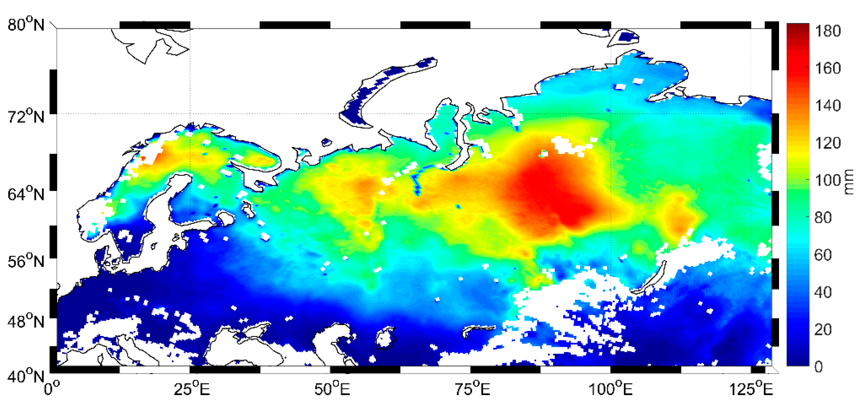
Figure 1 shows the spatial distribution pattern of the average winter SWE in Eurasia (40°N–80°N, 0°E–125°E). It can be seen that the distribution of SWE is geographically uneven. In general, SWE in high-latitude regions is higher than in mid-latitude regions. (The average SWE north of 60°N is 93.08 mm, whereas south of 60°N, it is 34.56 mm). In Siberia, SWE has significantly higher values than elsewhere. (The average SWE is 132.22 mm, 60°N–70°N, 75°E–100°E).
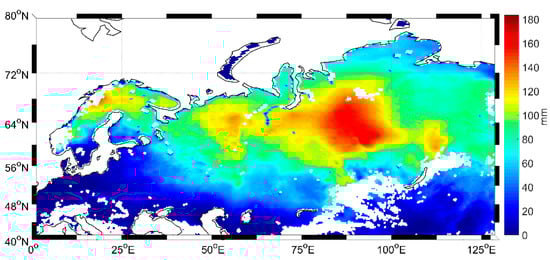
Figure 1.
The distribution characteristics of the average Eurasian snow water equivalent (SWE) in the winter during 1983–2018.
When studying the spatial characteristics of winter SWE in Eurasia, we used the empirical orthogonal function (EOF) to extract the spatial distribution characteristics and principal component time series (PCs) of the first two modes of Eurasian winter SWE.
Figure 2 shows the winter spatial distribution characteristics of the first mode and its PCs from 1983 to 2018. The SCF of the first mode measured 24.8% and passed the North test at a confidence level of 95%, indicating that EOF1 is sufficiently separate as to be non-degenerate. As Figure 2a shows, the main feature of the first mode is that winter SWE presents with an east–west dipole structure. The positive signal area is located in north Eurasia (centered at 62°N–64°N, 75°E–100°E), whereas the negative signal area is located in west Eurasia and is stronger than the positive signal (centered at 50°N–65°N, 25°E–65°E). These two areas are the key regions for changes in Eurasian winter SWE from 1983 to 2018. In Figure 2b, the PCs of the first mode exhibited interannual fluctuation characteristics and an upward trend and passed the M-K test at a confidence level of 95%, indicating that the upward trend is significant. Based on this finding, SWE is decreasing in the negative signal area of Eurasia but is increasing in the positive signal area in the north. The characteristics of the first mode are caused mainly by the warming of the North Atlantic Ocean, which promotes heavy snowfall in northern Eurasia and light snowfall in western Eurasia [32].
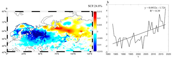
Figure 2.
(a) Spatial characteristics of the first mode of the empirical orthogonal Function for average Eurasian winter snow water equivalent (SWE) from 1983 to 2018; (b) principal component time series of the first mode of the empirical orthogonal function.
Figure 3 shows the spatial distribution characteristics of EOF2 and its PCs. The SCF of the second mode was 13.4% and passed the North test at a confidence level of 95%. As Figure 3a shows, Eurasian winter SWE presents a north–south dipole distribution. The positive signal area is located in northern Eurasia (center at 60°N–70°N, 55°E–125°E) and the negative signal area in the south of Eurasia (centered at 48°N–60°N, 10°E–100°E). The negative signal area presents discrete distribution characteristics, with a lower signal intensity than in the positive signal area. As Figure 3b shows, the PCs in the second mode show a downward trend in fluctuations that passes the M-K trend test at a confidence level of 95%, indicating that SWE is decreasing significantly in the positive signal area but growing rapidly in the negative signal area. In winter, interannual variations in SWE in Eurasia also showed a significant decreasing trend, with an average annual decrease of 0.19 mm. Additionally, interannual variations in Eurasian winter SWE were strongly correlated with the PCs of the first and second modes (with correlation coefficients of 0.56 and 0.51, respectively), indicating that interannual variations in Eurasian winter SWE are affected by the two modes. The distribution characteristics of the first mode cannot last until spring and are not correlated with autumn Arctic sea ice, so we primarily discuss the second mode of winter SWE in Eurasia.
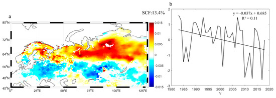
Figure 3.
(a) Spatial characteristics of the second mode of the empirical orthogonal function in average Eurasian winter snow water equivalent from 1983 to 2018; (b) principal component time series of the second mode of the empirical orthogonal function.
3.2. Effect of Autumn Arctic Sea Ice on Eurasian Winter SWE
Using the Hadley sea ice dataset, we calculated Arctic autumn SIC. To analyze the influence of autumn Arctic sea ice on winter SWE in Eurasia, we calculated the correlation coefficient between the PCs in the second mode and the Arctic autumn SIC. Before the correlation analysis, the two data types were detrended. We also calculated and noted the weak correlation coefficient between the PCs of the first mode and the autumn Arctic sea ice (only very fragmented areas passed the t-test at a confidence level of 95%).
Figure 4 shows the spatial distribution characteristics of the correlation coefficient between autumn Arctic SIC and the PCs of the second mode from 1983 to 2018. The colored part represents the high-correlation areas that passed the t-test at a confidence level of 95%. As Figure 4 shows, the Arctic sea ice and PCs of the second mode show a positive correlation in autumn, with areas of highly positive correlations concentrated in the Barents–Kara Seas (BKS), which has shown a notably rapid reduction in sea ice and can affect temperature, precipitation, and other climatic factors in the Northern Hemisphere [56,57,58,59]. To further analyze the influence of Arctic autumn SIC on winter SWE in Eurasia, we chose September, October, and November as the relevant months for calculating the correlation coefficient with the PCs of the second mode. The correlation coefficient between the Arctic SIC in September and the SWE in Eurasia showed a very discrete distribution, indicating that Arctic SIC in September has no significant effect on winter SWE. In October, the relevant areas are concentrated mainly in the high latitudes of the Kara Sea (81°N–83°N, 60°E–100°E), showing a positive correlation. In November, the relevant area expands to the high latitudes of the Barents Sea, with sea ice in most of the Kara Sea affecting Eurasian winter SWE (centered at 75°N–82°N, 40°E–100°E). Figure 4d shows the distribution of correlation coefficients between the average SIC from October to November and the PCs of the second mode. The correlation coefficients are concentrated in the entire Kara Sea and the high latitudes of the Barents Sea (75°N–85°N, 30°E–100°E).
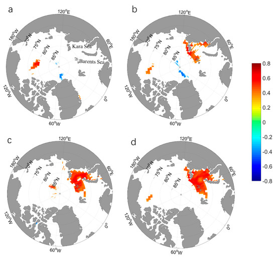
Figure 4.
(a) The correlation coefficient distribution between the principal component time series of the winter Eurasian snow water equivalent empirical orthogonal function mode 2 and autumn Arctic sea ice concentration in September, (b) October, (c) November, and (d) October–November. The colored regions passed the t-test with a confidence level of 95%. All of the series have been detrended.
We define the BKS average SIC time series in October–November as the BKS SIC index. To analyze the response of Eurasian winter SWE to BKS sea ice, we calculated the correlation coefficient distribution between the Eurasian winter SWE and the BSK SIC index. Prior to the analysis, all series were detrended.
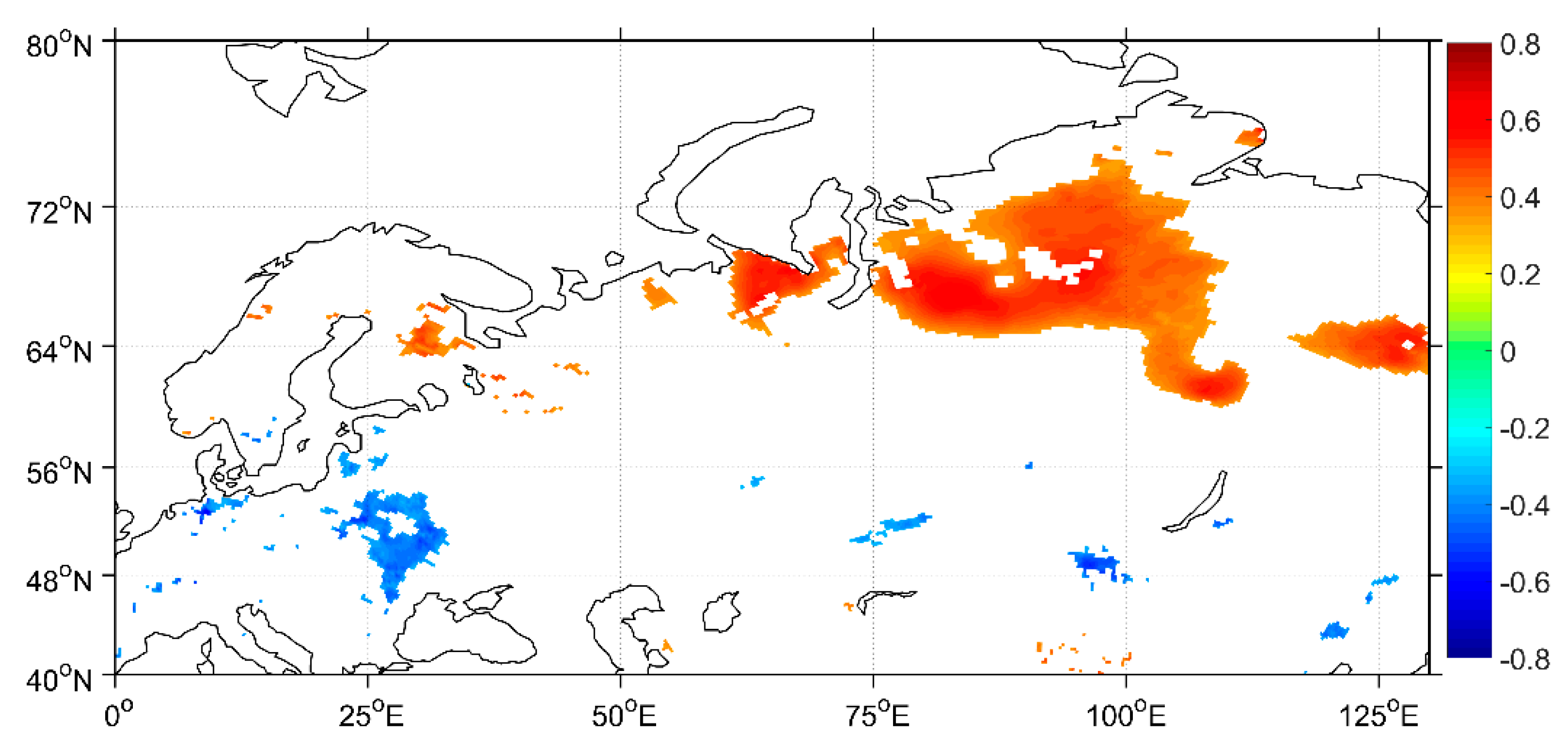
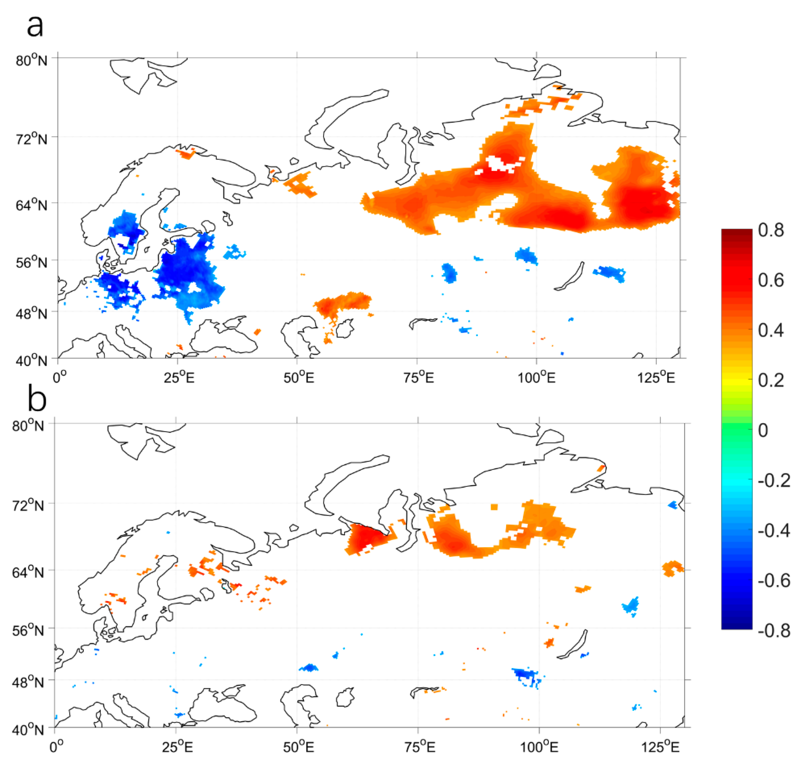
Figure 5 shows the distribution of the correlation coefficient between the BKS SIC index and Eurasian winter SWE from 1983 to 2018. The colored regions passed the t-test at a confidence level of 95%. The SWE of the two regions of Eurasia is highly correlated with the BKS SIC index. The positive area is located in northern Eurasia (centered at 64°N–72°N, 75°E–100°E), and the negative area is relatively discrete and is concentrated mainly in southwest Eurasia (centered at 48°N–56°N, 25°E–35°E). The distribution of the correlation coefficients in these two regions shows the characteristics of north–south dipole, and this structure has similar distribution characteristics to EOF2. This shows that BKS SIC is the key factor affecting the north–south distribution characteristics of winter SWE in Eurasia.
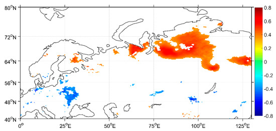
Figure 5.
The correlation coefficient distribution between winter snow water equivalent in Eurasia and the Barents–Karas Sea ice concentration index. The colored regions passed the t-test with a confidence level of 95%. All of the series have been detrended.
3.3. Effects of Autumn Arctic Sea Ice and Winter SWE on Spring SWE in Eurasia
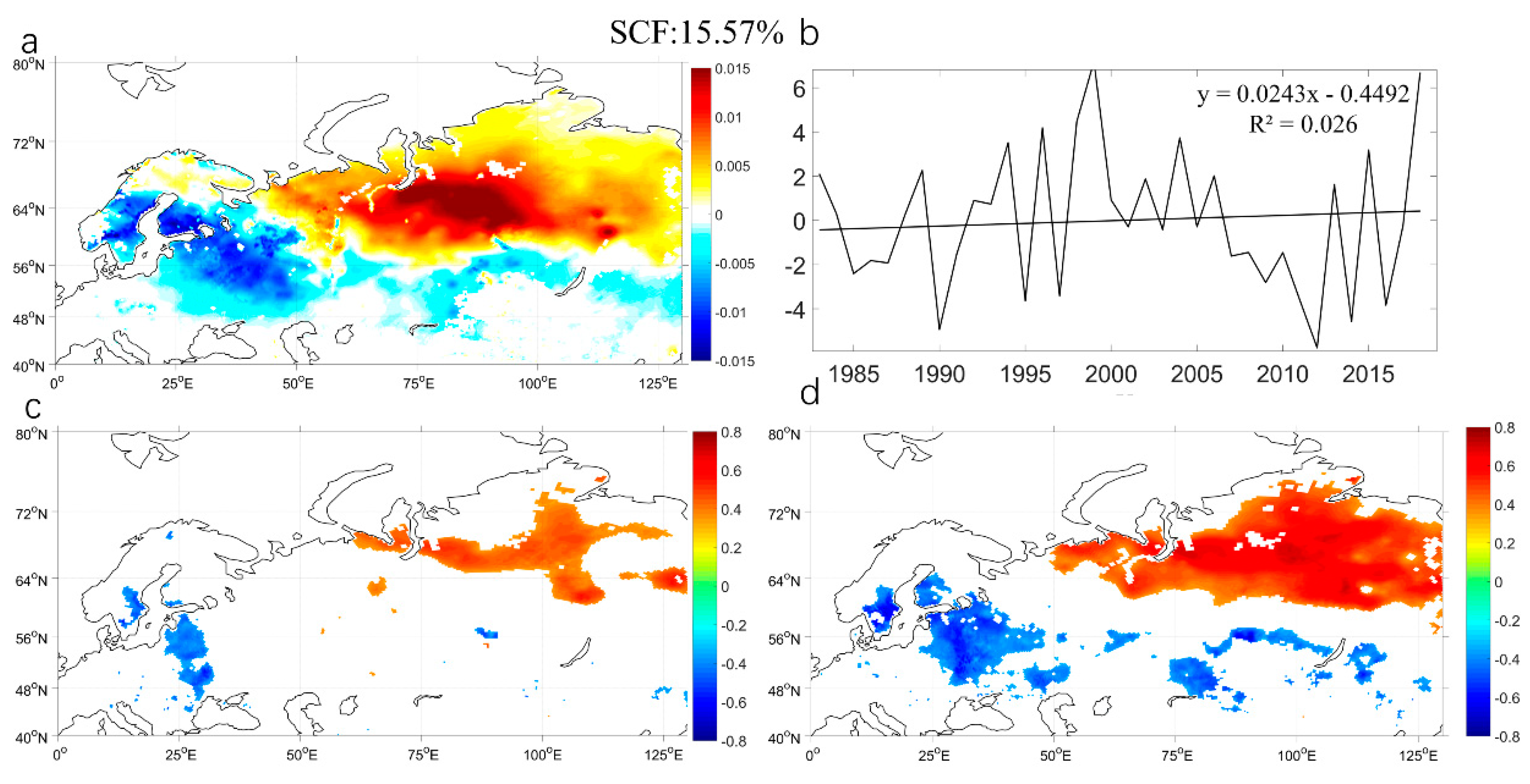
Figure 6a shows the spatial distribution characteristics of the first mode of Eurasian spring SWE. The SCF of the first mode is 15.57%. The first mode of Eurasian spring SWE is a dipole structure. The positive signal area is located in northern Eurasia and the negative signal area mainly in southwestern Eurasia, much as with the EOF2 of Eurasian winter SWE (the correlation coefficient between the two PCs is 0.85). Figure 6b shows the PCs of the first mode in spring, which exhibit a weak upward trend that did not pass the M-K test at a confidence level of 90%.

Figure 6.
(a) Spatial characteristics of the first mode of the empirical orthogonal function on average spring Eurasian snow water equivalent from 1983 to 2018; (b) principal component time series of the first mode of the empirical orthogonal function; (c) the correlation coefficient distribution between spring snow water equivalent in Eurasia and the Barents–Karas sea ice concentration index; (d) the correlation coefficient distribution between spring Eurasian snow water equivalent and the principal component time series of the empirical orthogonal function in winter Eurasian snow water equivalent.
To analyze the influence of Arctic BKS autumn sea ice on Eurasian spring SWE, we calculated the correlation coefficient between the BKS SIC index and Eurasian spring SWE. Before the calculation, all data were detrended. Figure 6c shows the distribution of the correlation coefficient between the BKS SIC index and spring SWE. The correlation coefficient also shows a dipole structure. The positive correlation area is located in northern Eurasia, and the negative correlation area is located in southwest Eurasia and has distribution characteristics similar to those of spring EOF1. This finding indicates that the influence of BKS autumn sea ice on Eurasian SWE will extend from winter to spring. Figure 6d shows the distribution of the correlation coefficients between the PCs of EOF2 for winter SWE in Eurasia and spring SWE. The distribution characteristics of the correlation coefficient also show a dipole structure, and the PCs of EOF2 of winter SWE have a stronger influence on spring SWE than the BKS index. The PCs of spring EOF1 may be the key to connecting BKS autumn sea ice and the spring SWE factor.
3.4. The Relationship between BKS Autumn Sea Ice and Winter–Spring Atmospheric Circulation
Studies have shown that the significant reduction of BKS autumn sea ice may cause changes in the atmospheric environment of the Northern Hemisphere, leading to abnormal circulation characteristics similar to the Siberian High (SH) (when BKS sea ice decreased, a positive SLP extended from BKS through Eastern Europe to Mongolia) and the Arctic Oscillation (AO) [60,61]. To analyze the influence of BKS SIC on winter atmospheric circulation in the Northern Hemisphere, we calculated the correlation coefficients between the BKS SIC index and winter sea level pressure (SLP) and 500 hpa geopotential height.
Figure 7a shows the correlation coefficient distribution between the BKS SIC index and winter SLP in the Northern Hemisphere. It can be seen that the SLP anomalies related to BKS SIC from October to November show a typical AO structure [62]. After detrending, the correlation between the BKS SIC index and the winter AO index is 0.46, indicating that BKS sea ice from October to November is closely related to winter AO. Figure 7b shows the distribution of the correlation coefficient between the BKS SIC index and the 500 pha geopotential height. In Figure 7b, the AO structure can still be seen, indicating that BKS SIC can still cause AO characteristics in the troposphere of the Northern Hemisphere [39].

Figure 7.
(a) The correlation coefficient distribution between the Barents–Karas sea ice concentration index and winter sea level pressure in the Northern Hemisphere; (b) the correlation coefficient distribution between Barents–Karas sea ice concentration index and winter 500 hpa geopotential height in the Northern Hemisphere. The colored regions passed the t-test with a confidence level of 95%. All of the series have been detrended.
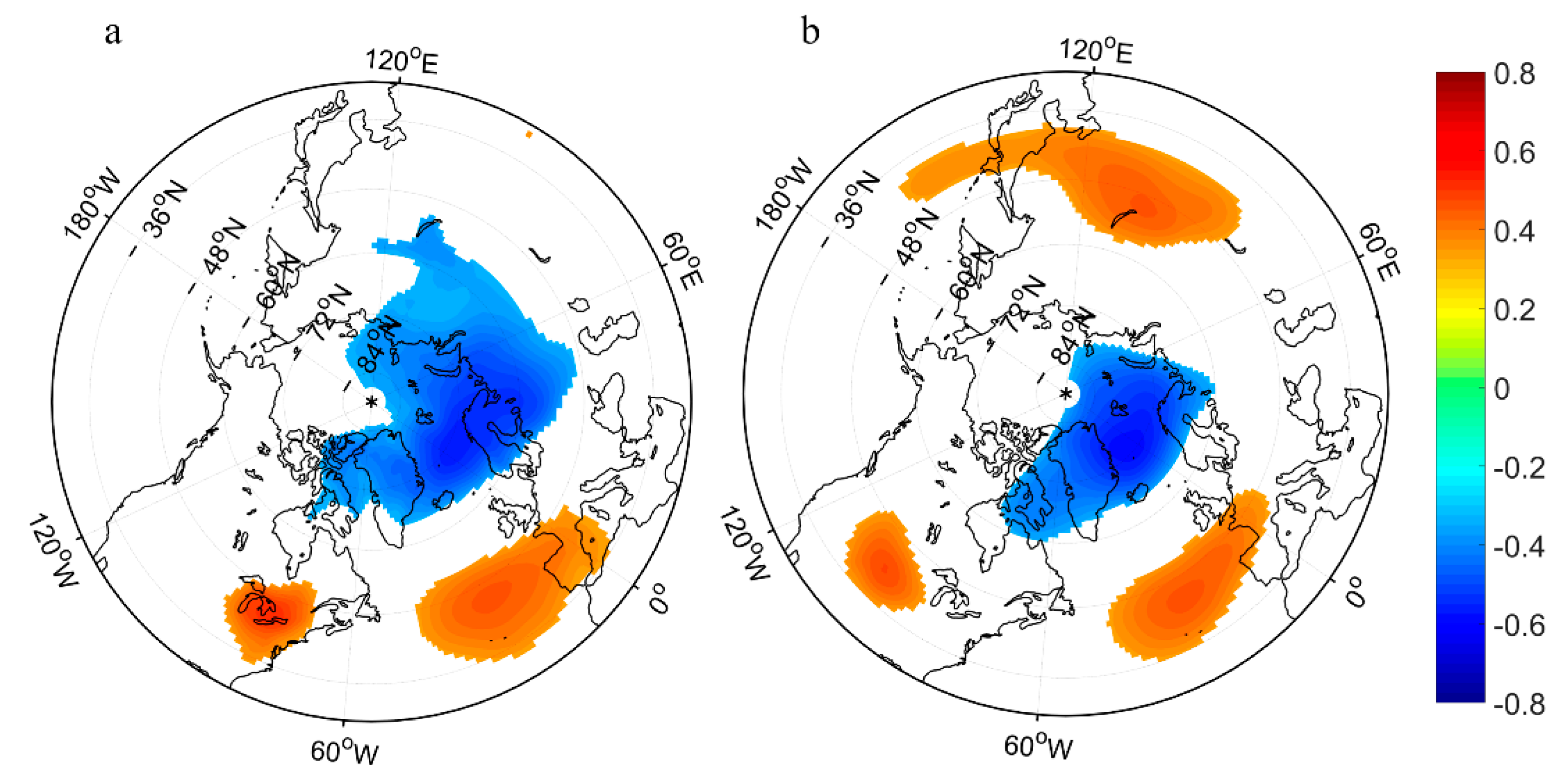
Figure 8a shows the correlation coefficient distribution between the winter AO index and the 500 hpa tropospheric potential height in November. The colored regions passed the t-test with a confidence level of 95%. It can be clearly seen from the figure that the tripolar structure has a negative signal in the BKS region, and positive signals in western Europe and eastern Eurasia. This structure is related to the activities of the Rossby wave [63]. Figure 8b shows the distribution of the high correlation coefficient between the BKS sea ice index in November and the 500 hpa tropospheric potential in November. In Eurasia, it shows similar distribution characteristics to Figure 8a. Autumn BKS sea ice, especially November BKS sea ice, is an important predictor of AO in winter [62,64]. As the BKS sea ice decreases, more open waters are created, which increases the local heat flux from the ocean to the atmosphere, and acts as a heat source for the overlying atmosphere [61]. In the BKS region, the response of the atmosphere to sea ice is generated by stable Rossby waves generated by the abnormal heat flux [63,64]. This Rossby wave is often regarded as a precursor to AO in winter [65,66]. With the propagation of this planetary wave, an anomaly of the tropospheric polar vortex circulation is formed, which is finally projected on the winter AO [67,68]. The AO started to form in December and stabilized until February [61,67]. During this period, the AO has a lasting effect on winter SWE.
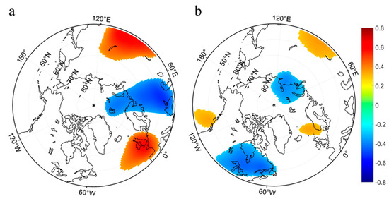
Figure 8.
(a) The correlation coefficient distribution between the winter Arctic Oscillation and November 500 hpa geopotential height; (b) the correlation coefficient distribution between the November Barents–Karas sea ice concentration index and November 500 hpa geopotential height. The colored regions passed the t-test with a confidence level of 95%. All of the series have been detrended.
AO is a key factor affecting climate change in Eurasia. Researchers have reported that AO can affect air temperature and precipitation in Eurasia [69,70]. To verify the effect of winter AO on Eurasian winter SWE, we calculated the correlation coefficient between the winter AO index and Eurasian winter SWE. Before calculation, all data were detrended. Figure 9a shows the distribution characteristics of the correlation coefficient between the winter AO index and Eurasian winter SWE. The colored regions passed the t-test at a confidence level of 95%. The Eurasian winter SWE related to winter AO also presents a north–south dipole distribution structure. The positive correlation area is concentrated in northern Eurasia, whereas the negative correlation area is concentrated mainly in southwest Eurasia. This indicates that when the winter AO is in a negative phase, winter SWE in northern Eurasia decreases (centered at 60°N–70°N, 75°E–125°E), whereas SWE in southwestern Eurasia increases (centered at 50°N–60°N, 20°E–35°E). The distribution structure of this SWE is similar to the second mode of Eurasian winter SWE (the correlation coefficient between PCs in the first mode of winter SWE and winter AO is 0.66) and the characteristics of the BKS SIC index that influence winter SWE. Accordingly, winter AO may be an important factor connecting BKS autumn sea ice and winter SWE. After using partial correlation analysis to ignore the influence of AO on Eurasian winter SWE, we calculated the partial correlation coefficient between the BKS SIC index and Eurasian winter SWE. As Figure 9b shows, when the influence of AO is ignored, the influence of the BKS SIC index on Eurasian SWE becomes weak, the positive correlation area in northern Eurasia shrinks, and the negative correlation area in the southwest disappears, further showing that winter AO is closely related to BKS SIC and Eurasian winter SWE.

Figure 9.
(a) The correlation coefficient distribution between the winter Arctic Oscillation and Eurasian winter snow water equivalent; (b) the partial correlation coefficient between the Barents–Karas sea ice concentration index and Eurasian winter snow water equivalent. The colored regions passed the t-test with a confidence level of 95%. All of the series have been detrended.
To study how the BKS SIC and EOF2 of Eurasian winter SWE affect Eurasian spring SWE, we first analyzed the role of spring AO. Table 1 shows the correlation coefficients between the spring AO index and the BKS SIC index, the second-mode PCs of Eurasian winter SWE, and the first-mode PCs of Eurasian spring SWE. The relationship between the BKS SIC index and winter AO is relatively weak (R = 0.21), so the winter AO characteristics caused by the decrease in the amount of BKS autumn sea ice cannot continue until spring. The AO related to BKS SIC forms in January and becomes stable in February as the polar vortex weakens, then disappears after March [61]. Whether for the PCs of the Eurasian winter SWE EOF2 or for the Eurasian spring SWE EOF1, the correlation with the spring AO index is very weak (correlation coefficients of 0.12 and 0.14, respectively), indicating that atmospheric circulation might not be the main factor affecting changes to Eurasian spring SWE.

Table 1.
Correlation coefficients between the spring Arctic Oscillation and the Barents–Karas sea ice concentration index, principal component time series of Eurasian snow water equivalent EOF2 in winter, and principal component time series of Eurasian snow water equivalent EOF1 in spring.
3.5. Dynamic Process
Generally speaking, temperature and precipitation are the two main factors affecting snow cover [39,71]. Based on Figure 3a, which shows the distribution pattern of the winter SWE of EOF2, we selected SWE in northern Eurasia (centered at 60°N–70°N, 55°E–125°E) as well as in southwestern Eurasia (centered at 48°N–60°N, 10°E–30°E), analyzing the effects of precipitation and temperature.
Table 2 shows the relationship between winter SWE and winter precipitation, winter air temperature at 2 m, winter AO in winter, and BKS autumn SIC. In northern Eurasia, winter SWE is strongly correlated with precipitation and air temperature, with correlation coefficients of 0.60 and 0.58, respectively. Calculating the average air temperature at 2 m reveals that the average 2 m air temperature in northern Eurasia in winter is −25.3 °C, with a standard deviation of 2.8 °C—much lower than the freezing temperature. As a result, northern Eurasian temperatures might not be a key factor affecting local snow cover. In southwest Eurasia, the correlation between SWE and winter precipitation is very low (R = −0.20), but there is a high correlation between air temperature at 2 m and SWE (R = −0.87). The average air temperature at 2 m in southwest Eurasia is −1.3 °C and the standard deviation is 1.99 °C, indicating that the temperature at 2 m fluctuates around 0 °C. Thus, temperature changes might be an important factor in local snow cover changes.
Table 2.
Correlation coefficients between Eurasian snow water equivalent and precipitation, air temperature at 2 m, the Arctic Oscillation in winter and the autumn Barents–Karas sea ice concentration index.
To study the path by which BKS autumn SIC influences Eurasian winter SWE, we calculated the correlation coefficient between the BKS SIC index and winter integrated water vapor flux. All data were detrended before calculation. Figure 10a shows the distribution characteristics of the correlation coefficient between the BKS SIC index and integrated zonal water vapor flux. The colored regions passed the t-test with a confidence level of 95%. In Figure 10a, the positive correlation area represents the water vapor flux from north to south, and vice versa for the negative correlation area. In northern Eurasia, a north–south zonal water vapor flux can be seen connecting the Arctic seas and Eurasia, indicating that when BKS SIC increases in autumn, zonal water vapor flux brings water vapor from the Arctic to northern Eurasia, which promotes snowfall and increases SWE under cold conditions in the north. When BKS SIC decreases in the autumn, the zonal water vapor flux weakens and Eurasian winter SWE decreases. Figure 9b shows the distribution characteristics of the correlation coefficient between the BKS SIC index and integrated meridional water vapor flux. In Figure 10b, the negative correlation area represents the integrated meridional water vapor flux from west to east related to BKS sea ice, and vice versa for the positive correlation area. When BKS sea ice decreases, west–east water vapor flux in the north Atlantic increases, encouraging warm, humid water vapor to enter northern and southwestern Eurasia, increasing southwest Eurasian precipitation and temperature. Although the southwestern Eurasian temperature has risen, the region is still cold. The average air temperature in the local area in winter is still below freezing in most years, which promotes snowfall. In addition, because warm air is conducive to providing more water vapor, southwestern Eurasian SWE has increased [26,27,39]. In northern Eurasia, large-scale east–west water vapor flux is related to BKS sea ice. Although east–west water vapor transport weakens when BKS sea ice decreases, it can still hinder the passage of warmth and wet water vapor from the Atlantic Ocean, so northern Eurasian temperatures are lower than in the southwest, with less snowfall. Figure 10c shows that when BKS sea ice is low, integrated water vapor transport is abnormal in the Eurasian region. When BKS sea ice is low, water vapor flux from the Arctic is very small, hindering snowfall in Eurasia. Strong cyclones in the North Atlantic encourage water vapor to enter southwestern Eurasia from the North Atlantic, increasing the temperature and snowfall. In most of northern Eurasia, water vapor flux from the Arctic seas to Eurasia is weakened. In addition, abnormal east–west water vapor flux characteristics prevent water vapor from the North Atlantic from entering northern Eurasia. These factors are not conducive to snowfall in northern Eurasia, helping maintain cooler air in the north.
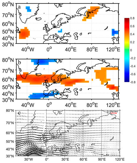
Figure 10.
(a) The correlation coefficient distribution between the Barents–Karas sea ice concentration index and integrated zonal water vapor flux: (b) the correlation coefficient distribution between the Barents–Karas sea ice concentration index and winter integrated meridional water vapor flux. The colored regions passed the t-test with a confidence level of 95%. All of the series have been detrended. (c) The abnormal winter water vapor flux when the Barents–Karas sea ice concentration sea ice is at a low value, unit: kg m−1s−1.
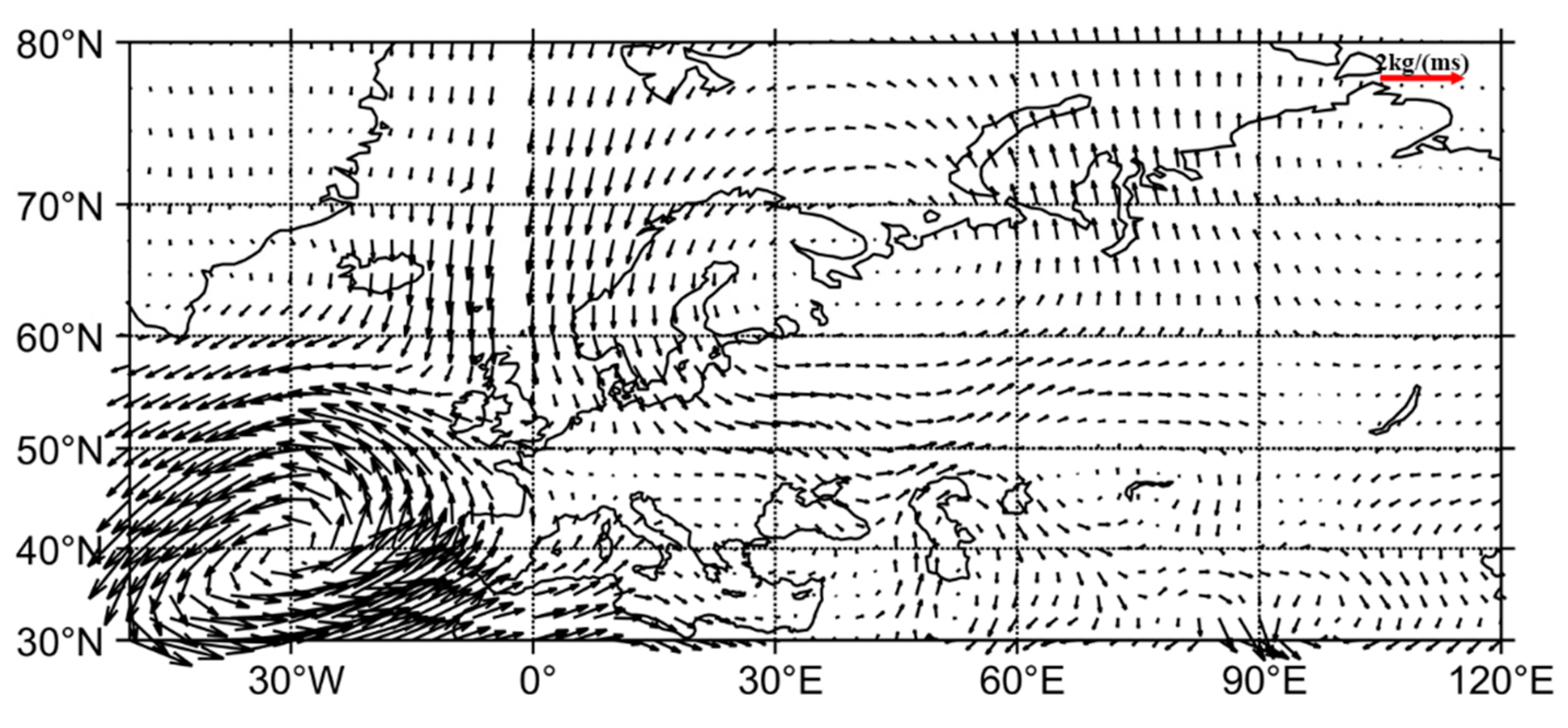
Figure 11 shows abnormal spring water vapor transport in Eurasia when BKS sea ice is low. In spring, no water vapor flux from the Arctic enters Eurasia through the BKS. Because the flux of water vapor from the North Atlantic into southwestern Eurasia is also significantly weakened, spring atmospheric circulation characteristics related to BKS sea ice do not significantly influence Eurasian spring SWE, with water vapor flux caused by BKS sea ice leading to changes in precipitation and temperature, weakly influencing levels of SWE. When analyzing the relationship between spring Eurasian surface temperature and winter–spring SWE, Zhang et al. found that if the spring SWE signal was deleted, the relationship between autumn SIC and winter Eurasian SWE and spring SWE would be very weak, which also suggested that spring SWE distribution may be caused by winter SWE memory [34].
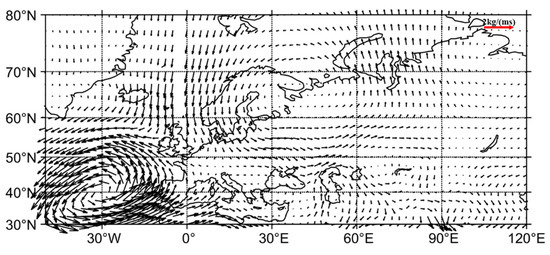
Figure 11.
The abnormal spring water vapor flux when the Barents–Karas sea ice concentration is at a low value, unit: kg m−1s−1.
3.6. Predicted Eurasian Winter–Spring SWE
Changes to Eurasian winter and spring SWE can affect vegetation, temperature, and other factors [72,73,74], so correctly predicting changes to Eurasian winter and spring SWE is important. In the previous analysis, we found that BKS SIC affects Eurasian winter and spring SWE. Using a linear regression model and support vector machine (SVM) regression, we used BKS autumn SIC to predict Eurasian winter and spring SWE. In Lindsay’s method [68], the first step is to calculate the correlation coefficient between SWE time series and Arctic sea ice so as to obtain the correlation coefficient matrix. In the second step, the SIC matrix is multiplied by the correlation coefficient matrix, after which the average value is calculated to obtain the time series of the predictive factors. We use data from 1983 to 1999 to train a regression model, then use the model to predict SWE from 2000 to 2018. We chose the root mean square error (RMSE) and the average absolute error (MAE) as the evaluation indicators.
Table 3 compares the predicted and actual values of Eurasian winter and spring SWE between 2000 and 2018. Whether analyzed using a linear regression or the support vector machine, BKS autumn SIC has a relatively good predictive ability for Eurasian winter SWE, with a correlation coefficient (R) of 0.75 and RMSE around 3.24 mm, indicating that BKS autumn SIC can be used to predict Eurasian winter SWE. In spring, the predictions of the SVM model outperform those of linear regression. In general, the predictive ability of BKS autumn SIC for Eurasian spring SWE is relatively weak, with an R of 0.43 and an RMSE of about 4.48 mm.
Table 3.
Comparison of forecasted values and actual results of Eurasian SWE in autumn and winter from 2000 to 2018.
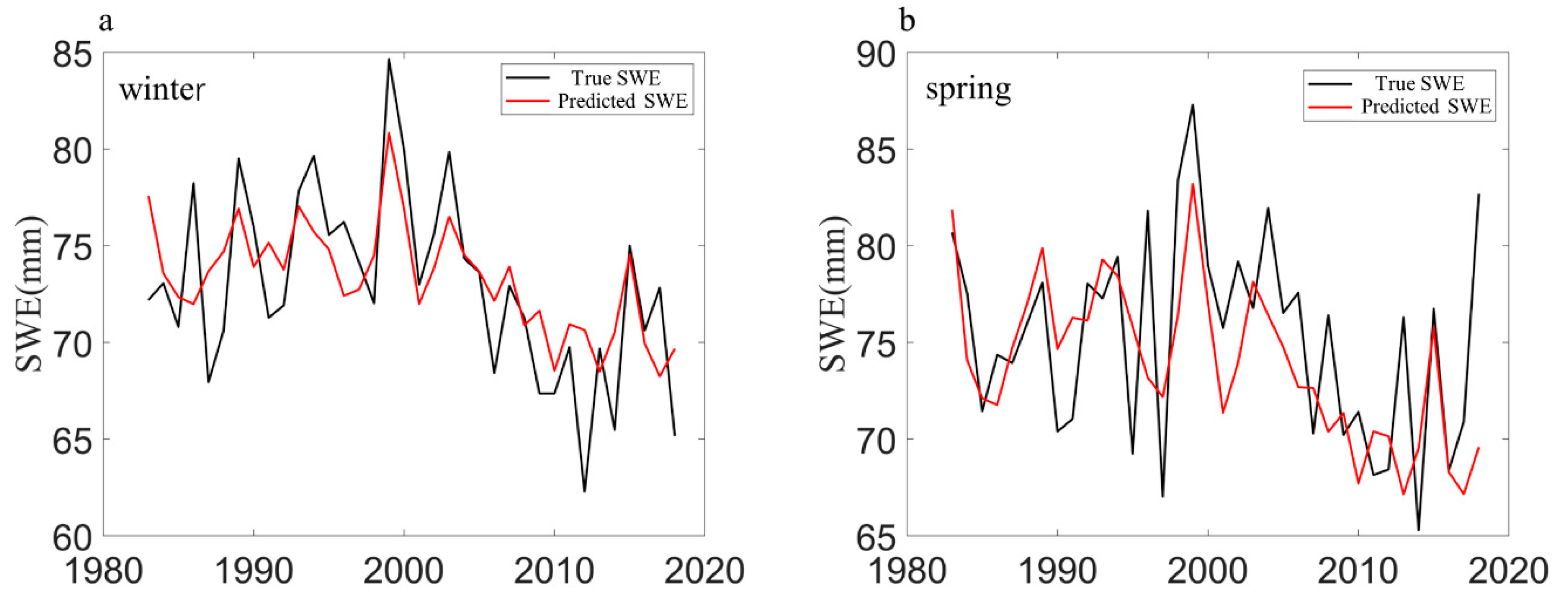
Figure 12 compares the empirical prediction model with actual values from 1983 to 2018. Generally, the two show similar fluctuation characteristics. In winter, the correlation coefficient between the two after detrending is 0.65, versus 0.56 in spring. Eurasian spatial distribution characteristics in winter and spring are complex and are closely related to changes in north Atlantic sea surface temperature, local atmospheric circulation, and thermodynamic conditions [75,76,77]. In the next step, further analysis of factors related to Eurasian SWE is needed to establish a higher-precision prediction model.
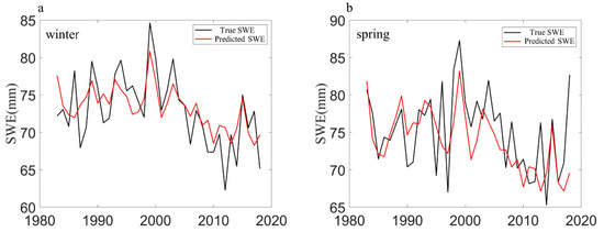
Figure 12.
(a,b) Comparison of the forecast results and actual values of the Eurasian winter–spring SWE from 1983 to 2018. The result from 1983 to 1999 is the training data and 2000–2018 is the forecast.
4. Conclusions
SWE is an important part of the surface energy and water cycle, influencing global climate change. We studied the spatial distribution characteristics of Eurasian SWE and its relationship with Arctic sea ice. As expected, our results are consistent with previous findings, indicating that changes in Eurasian SWE are closely related to reductions in sea ice and water vapor flux [77,78]. Generally speaking, SWE is highest in Siberia, with Eurasian SWE distributed more northernly and less southernly, much as reported by Zhang et al. [76]. The most direct impact on Eurasian SWE comes from temperature and water vapor transport, with the SWE in northern Eurasian less affected by temperature but the SWE in southern Eurasian more affected by temperature, again consistent with the findings of Zhong et al. [21].
In this study, we explored changes in Eurasian winter and spring SWE and their relationship with autumn Arctic sea ice and atmospheric circulation in the Northern Hemisphere. We found that the first mode of Eurasian winter SWE presents an east–west dipole distribution, with SWE in the west significantly reduced and SWE in the east significantly increased—findings related to the warm North Atlantic SST. The second mode shows that Eurasian winter SWE presents a north–south dipole distribution, with SWE in the north significantly reduced and SWE in the south significantly increased. Both the first and second modes are strongly correlated with Eurasian winter SWE.
BKS SIC is significantly related to the north–south distribution characteristics of Eurasian winter SWE. The second mode of Eurasian winter SWE has the weakest relationship with September BKS SIC and the strongest relationship with November BKS SIC. BKS SIC affects mainly winter SWE in northern and southwestern Eurasia, with its influence on Eurasian SWE potentially continuing into spring. The first mode of Eurasian spring SWE presents a north–south dipole distribution and is significantly related to the second mode of winter SWE and BKS autumn SIC, indicating that Eurasian winter SWE may be an important factor connecting BKS autumn SIC and spring SWE.
Changes to BKS autumn SIC can trigger an Arctic Oscillation (AO) characteristic winter atmospheric circulation anomaly that also causes the north–south dipole distribution in Eurasian winter SWE. When ignoring the influence of AO, the influence of BKS autumn SIC on winter SWE became very weak, indicating that AO may be the key factor connecting BKS autumn SIC with Eurasian winter SWE. However, the spring AO related to BKS SIC had no significant effect on Eurasian spring SWE, and atmospheric circulation might not be a key factor affecting Eurasian spring SWE.
The analysis of precipitation and temperature in Eurasia revealed that changes in the SWE in northern Eurasia in winter are closely related to precipitation, with SWE in the southwest closely related to temperature. The analysis of integrated water vapor transport revealed that when BKS autumn SIC is low, water vapor transport from the Arctic seas is weakened, hindering accumulation and maintenance of SWE. In the North Atlantic, strong meridional water vapor transport brings warm, humid water vapor to southwestern Eurasia, encouraging accumulation of SWE. Zonal water vapor transport in northern Eurasia prevents water vapor transport in the Atlantic Ocean from entering northern Eurasian, which hinders accumulation of northern Eurasian SWE while preserving the cold climate. Changes in Eurasian spring SWE mainly reflect the memory effect of winter SWE.
BKS autumn SIC can be used to predict Eurasian SWE, with the R value peaking at 0.75. For spring SWE, however, BKS autumn SIC has weak predictability. Changes in Eurasian SWE are complex and are related to sea temperature, local atmospheric circulation, and thermodynamic factors. Future research should further analyze the temporal and spatial distribution characteristics of Eurasian SWE and its relationship with other elements with a view to devising a more precise forecasting model.
Author Contributions
Conceptualization, J.F. and Y.Z.; methodology, J.F.; software, J.F.; validation, K.W., J.F. and Y.Z.; formal analysis, J.F.; investigation, K.W.; resources, J.Y.T.; data curation, J.F.; writing—original draft preparation, J.F. and Y.Z.; writing—review and editing, Y.Z.; visualization, K.W.; supervision, Y.Z.; project administration, J.Y.T.; funding acquisition, Y.Z. All authors have read and agreed to the published version of the manuscript.
Funding
This research was funded by the National Natural Science Foundation (U1901215), the Marine Special Program of Jiangsu Province in China (JSZRHYKJ202007), and the Natural Scientific Foundation of Jiangsu Province (BK20181413).
Acknowledgments
The GlobSnowv3.0 data and the ECMWF Reanalysis data are highly appreciated. This research was supported by the National Natural Science Foundation (U1901215), the Marine Special Program of Jiangsu Province in China (JSZRHYKJ202007), and the Natural Scientific Foundation of Jiangsu Province (BK20181413).
Conflicts of Interest
The authors declare no conflict of interest.
References
- Laine, V. Arctic sea ice regional albedo variability and trends, 1982–1998. J. Geophys. Res. Ocean. 2004, 109. [Google Scholar] [CrossRef]
- Peng, H.T.; Ke, C.Q.; Shen, X.; Li, M.; Shao, Z.D. Summer albedo variations in the Arctic sea ice region from 1982 to 2015. Int. J. Climatol. 2020, 40, 3008–3020. [Google Scholar] [CrossRef]
- Stroeve, J.C.; Serreze, M.C.; Holland, M.M.; Kay, J.E.; Malanik, J.; Barrett, A.P. The Arctic’s rapidly shrinking sea ice cover: A research synthesis. Clim. Chang. 2012, 110, 1005–1027. [Google Scholar] [CrossRef] [Green Version]
- Maslanik, J.A.; Fowler, C.; Stroeve, J.; Drobot, S.; Zwally, J.; Yi, D.; Emery, W. A younger, thinner Arctic ice cover: Increased potential for rapid, extensive sea-ice loss. Geophys. Res. Lett. 2007, 34. [Google Scholar] [CrossRef] [Green Version]
- Bader, J.; Mesquita, M.D.S.; Hodges, K.I.; Keenlyside, N.; Østerhus, S.; Miles, M. A review on Northern Hemisphere sea-ice, storminess and the North Atlantic Oscillation: Observations and projected changes. Atmos. Res. 2011, 101, 809–834. [Google Scholar] [CrossRef]
- Comiso, J.C.; Parkinson, C.L.; Gersten, R.; Stock, L. Accelerated decline in the Arctic sea ice cover. Geophys. Res. Lett. 2008, 35, L01703. [Google Scholar] [CrossRef] [Green Version]
- Cavalieri, D.J.; Parkinson, C.L. Arctic sea ice variability and trends, 1979–2010. Cryosphere 2012, 6, 881. [Google Scholar] [CrossRef] [Green Version]
- Comiso, J.C.; Meier, W.N.; Gersten, R. Variability and trends in the Arctic Sea ice cover: Results from different techniques. J. Geophys. Res. Ocean. 2017, 122, 6883–6900. [Google Scholar] [CrossRef]
- Fan, K. North Pacific sea ice cover, a predictor for the Western North Pacific typhoon frequency? Sci. China Ser. D Earth Sci. 2007, 50, 1251–1257. [Google Scholar] [CrossRef]
- Vihma, T. Effects of Arctic sea ice decline on weather and climate: A review. Surv. Geophys. 2014, 35, 1175–1214. [Google Scholar] [CrossRef] [Green Version]
- McCusker, K.E.; Kushner, P.J.; Fyfe, J.C.; Sigmond, M.; Kharin, V.V.; Bitz, C.M. Remarkable separability of circulation response to Arctic sea ice loss and greenhouse gas forcing. Geophys. Res. Lett. 2017, 44, 7955–7964. [Google Scholar] [CrossRef]
- Wu, Z.; Li, X.; Li, Y.; Li, Y. Potential influence of Arctic sea ice to the interannual variations of East Asian spring precipitation. J. Clim. 2016, 29, 2797–2813. [Google Scholar] [CrossRef]
- Gao, Y.; Sun, J.; Li, F.; He, S.; Sandven, S.; Yan, Q.; Suo, L. Arctic sea ice and Eurasian climate: A review. Adv. Atmos. Sci. 2015, 32, 92–114. [Google Scholar] [CrossRef] [Green Version]
- Zuo, J.; Ren, H.L.; Wu, B.; Li, W. Predictability of winter temperature in China from previous autumn Arctic sea ice. Clim. Dyn. 2016, 47, 2331–2343. [Google Scholar] [CrossRef]
- Tang, Q.; Zhang, X.; Yang, X.; Francis, J.A. Cold winter extremes in northern continents linked to Arctic sea ice loss. Environ. Res. Lett. 2013, 8, 014036. [Google Scholar] [CrossRef]
- Sun, C.; Yang, S.; Li, W.; Zhang, R.; Wu, R. Interannual variations of the dominant modes of East Asian winter monsoon and possible links to Arctic sea ice. Clim. Dyn. 2016, 47, 481–496. [Google Scholar] [CrossRef]
- Na, L.; Jiping, L.; Zhanhai, Z.; Hongxia, C.; Mirong, S. Is extreme Arctic sea ice anomaly in 2007 a key contributor to severe January 2008 snowstorm in China? Int. J. Climatol. 2012, 32, 2081–2087. [Google Scholar] [CrossRef]
- Liu, Y.; Ren, H.L. A hybrid statistical downscaling model for prediction of winter precipitation in China. Int. J. Climatol. 2015, 35, 1309–1321. [Google Scholar] [CrossRef]
- Nayak, A.; Marks, D.; Chandler, D.G.; Seyfried, M. Long-term snow, climate, and streamflow trends at the Reynolds Creek experimental watershed, Owyhee Mountains, Idaho, United States. Water Resour. Res. 2010, 46. [Google Scholar] [CrossRef]
- Lazar, B.; Williams, M. Climate change in western ski areas: Potential changes in the timing of wet avalanches and snow quality for the Aspen ski area in the years 2030 and 2100. Cold Reg. Sci. Technol. 2008, 51, 219–228. [Google Scholar] [CrossRef]
- Zhong, X.; Zhang, T.; Kang, S.; Wang, K.; Zheng, L.; Hu, Y.; Wang, H. Spatiotemporal variability of snow depth across the Eurasian continent from 1966 to 2012. Cryosphere 2018, 12, 227. [Google Scholar] [CrossRef] [Green Version]
- Wang, L.; Chen, W. The East Asian winter monsoon: Re-amplification in the mid-2000s. Chin. Sci. Bull. 2014, 59, 430–436. [Google Scholar] [CrossRef]
- Jia, X.; Cao, D.R.; Ge, J.W.; Wang, M. Interdecadal change of the impact of Eurasian snow on spring precipitation over southern China. J. Geophys. Res. Atmos. 2018, 123, 10092–10108. [Google Scholar] [CrossRef]
- Zhang, T.; Wang, T.; Krinner, G.; Wang, X.; Gasser, T.; Peng, S.; Yao, T. The weakening relationship between Eurasian spring snow cover and Indian summer monsoon rainfall. Sci. Adv. 2019, 5, eaau8932. [Google Scholar] [CrossRef] [Green Version]
- Brown, R.D.; Robinson, D.A. Northern Hemisphere spring snow cover variability and change over 1922–2010 including an assessment of uncertainty. Cryosphere 2011, 5, 219. [Google Scholar] [CrossRef] [Green Version]
- Ye, H.; Cho, H.R.; Gustafson, P.E. The changes in Russian winter snow accumulation during 1936–1983 and its spatial patterns. J. Clim. 1998, 11, 856–863. [Google Scholar] [CrossRef]
- Kitaev, L.; Førland, E.; Razuvaev, V.; Tveito, O.E.; Krueger, O. Distribution of snow cover over Northern Eurasia. Hydrol. Res. 2005, 36, 311–319. [Google Scholar] [CrossRef]
- Seager, R.; Kushnir, Y.; Nakamura, J.; Ting, M.; Naik, N. Northern Hemisphere winter snow anomalies: ENSO, NAO and the winter of 2009/10. Geophys. Res. Lett. 2010, 37. [Google Scholar] [CrossRef] [Green Version]
- Kim, Y.; Kim, K.Y.; Kim, B.M. Physical mechanisms of European winter snow cover variability and its relationship to the NAO. Clim. Dyn. 2013, 40, 1657–1669. [Google Scholar] [CrossRef]
- Sun, C.; Zhang, R.; Li, W.; Zhu, J.; Yang, S. Possible impact of North Atlantic warming on the decadal change in the dominant modes of winter Eurasian snow water equivalent during 1979–2015. Clim. Dyn. 2019, 53, 5203–5213. [Google Scholar] [CrossRef]
- Cohen, J.; Jones, J.; Furtado, J.C.; Tziperman, E. Warm Arctic, cold continents: A common pattern related to Arctic sea ice melt, snow advance, and extreme winter weather. Oceanography 2013, 26, 150–160. [Google Scholar] [CrossRef]
- O’Gorman, P.A. Contrasting responses of mean and extreme snowfall to climate change. Nature 2014, 512, 416–418. [Google Scholar] [CrossRef] [Green Version]
- Handorf, D.; Jaiser, R.; Dethloff, K.; Rinke, A.; Cohen, J. Impacts of Arctic sea ice and continental snow cover changes on atmospheric winter teleconnections. Geophys. Res. Lett. 2015, 42, 2367–2377. [Google Scholar] [CrossRef] [Green Version]
- Zhang, R.; Sun, C.; Zhang, R.; Li, W.; Zuo, J. Role of Eurasian snow cover in linking winter-spring Eurasian coldness to the autumn Arctic sea ice retreat. J. Geophys. Res. Atmos. 2019, 124, 9205–9221. [Google Scholar] [CrossRef] [Green Version]
- Barnett, T.P.; Adam, J.C.; Lettenmaier, D.P. Potential impacts of a warming climate on water availability in snow-dominated regions. Nature 2005, 438, 303–309. [Google Scholar] [CrossRef] [PubMed]
- Peng, S.; Piao, S.; Ciais, P.; Fang, J.; Wang, X. Change in winter snow depth and its impacts on vegetation in China. Glob. Chang. Biol. 2010, 16, 3004–3013. [Google Scholar] [CrossRef]
- Blankinship, J.C.; Meadows, M.W.; Lucas, R.G.; Hart, S.C. Snowmelt timing alters shallow but not deep soil moisture in the Sierra Nevada. Water Resour. Res. 2014, 50, 1448–1456. [Google Scholar] [CrossRef]
- Gastineau, G.; García-Serrano, J.; Frankignoul, C. The influence of autumnal Eurasian snow cover on climate and its link with Arctic sea ice cover. J. Clim. 2017, 30, 7599–7619. [Google Scholar] [CrossRef]
- Xu, B.; Chen, H.; Gao, C.; Zhou, B.; Sun, S.; Zhu, S. Regional response of winter snow cover over the Northern Eurasia to late autumn Arctic sea ice and associated mechanism. Atmos. Res. 2019, 222, 100–113. [Google Scholar] [CrossRef]
- Takala, M.; Luojus, K.; Pulliainen, J.; Derksen, C.; Lemmetyinen, J.; Kärnä, J.P.; Bojkov, B. Estimating northern hemisphere snow water equivalent for climate research through assimilation of space-borne radiometer data and ground-based measurements. Remote Sens. Environ. 2011, 115, 3517–3529. [Google Scholar] [CrossRef]
- Pulliainen, J. Mapping of snow water equivalent and snow depth in boreal and sub-arctic zones by assimilating space-borne microwave radiometer data and ground-based observations. Remote Sens. Environ. 2006, 101, 257–269. [Google Scholar] [CrossRef]
- Kelly, R.E.; Chang, A.T.; Tsang, L.; Foster, J.L. A prototype AMSR-E global snow area and snow depth algorithm. IEEE Trans. Geosci. Remote Sens. 2003, 41, 230–242. [Google Scholar] [CrossRef] [Green Version]
- Bormann, K.J.; Brown, R.D.; Derksen, C.; Painter, T.H. Estimating snow-cover trends from space. Nat. Clim. Chang. 2018, 8, 924–928. [Google Scholar] [CrossRef]
- Pulliainen, J.; Luojus, K.; Derksen, C.; Mudryk, L.; Lemmetyinen, J.; Salminen, M.; Norberg, J. Patterns and trends of Northern Hemisphere snow mass from 1980 to 2018. Nature 2020, 581, 294–298. [Google Scholar] [CrossRef] [PubMed]
- Adler, R.F.; Huffman, G.J.; Chang, A.; Ferraro, R.; Xie, P.P.; Janowiak, J.; Nelkin, E. The version-2 global precipitation climatology project (GPCP) monthly precipitation analysis (1979–present). J. Hydrometeorol. 2003, 4, 1147–1167. [Google Scholar] [CrossRef]
- Pearson, K. Note on regression and inheritance in the case of two parents. Proc. R. Soc. Lond. 1895, 58, 240–242. [Google Scholar]
- Fleiss, J.L.; Tanur, J.M. A note on the partial correlation coefficient. Am. Stat. 1971, 25, 43–45. [Google Scholar]
- Raffalovich, L.E. Detrending time series: A cautionary note. Sociol. Metod. Res. 1994, 22, 492–519. [Google Scholar] [CrossRef]
- Weare, B.C.; Nasstrom, J.S. Examples of extended empirical orthogonal function analyses. Mon. Weather. Rev. 1982, 110, 481–485. [Google Scholar] [CrossRef]
- North, G.R.; Bell, T.L.; Cahalan, R.F.; Moeng, F.J. Sampling Errors in the Estimation of Empirical Orthogonal Functions. Mon. Weather. Rev. 1982, 110, 699. [Google Scholar] [CrossRef]
- Trenberth, K.E. Climate diagnostics from global analyses: Conservation of mass in ECMWF analyses. J. Clim. 1991, 4, 707–722. [Google Scholar] [CrossRef] [Green Version]
- Yue, S.; Wang, C.Y. The Mann-Kendall test modified by effective sample size to detect trend in serially correlated hydrological series. Water Resour. Manag. 2004, 18, 201–218. [Google Scholar] [CrossRef]
- Mann, H.B. Nonparametric tests against trend. Econom. J. Econom. Soc. 1945, 13, 245–259. [Google Scholar] [CrossRef]
- Kendall, M.G. Rank Correlation Methods; Griffin: Santa Barbara, CA, USA, 1948. [Google Scholar]
- Awad, M.; Khanna, R. Support Vector Regression. Efficient Learning Machines; Apress: Berkeley, CA, USA, 2015; pp. 67–80. [Google Scholar]
- Onarheim, I.H.; Eldevik, T.; Smedsrud, L.H.; Stroeve, J.C. Seasonal and regional manifestation of Arctic sea ice loss. J. Clim. 2018, 31, 4917–4932. [Google Scholar] [CrossRef]
- Screen, J.A.; Simmonds, I. The central role of diminishing sea ice in recent Arctic temperature amplification. Nature 2010, 464, 1334–1337. [Google Scholar] [CrossRef] [Green Version]
- Li, F.; Wang, H. Autumn sea ice cover, winter Northern Hemisphere annular mode, and winter precipitation in Eurasia. J. Clim. 2012, 26, 3968–3981. [Google Scholar] [CrossRef]
- Mori, M.; Kosaka, Y.; Watanabe, M.; Nakamura, H.; Kimoto, M. A reconciled estimate of the influence of Arctic sea-ice loss on recent Eurasian cooling. Nat. Clim. Chang. 2019, 9, 123–129. [Google Scholar] [CrossRef]
- Lü, Z.; He, S.; Li, F.; Wang, H. Impacts of the autumn Arctic sea ice on the intraseasonal reversal of the winter Siberian High. Adv. Atmos. Sci. 2019, 36, 173–188. [Google Scholar] [CrossRef] [Green Version]
- Yang, X.Y.; Yuan, X.; Ting, M. Dynamical link between the Barents–Kara sea ice and the Arctic Oscillation. J. Clim. 2016, 29, 5103–5122. [Google Scholar] [CrossRef]
- Deser, C.; Tomas, R.; Alexander, M.; Lawrence, D. The seasonal atmospheric response to projected Arctic sea ice loss in the late twenty-first century. J. Clim. 2010, 23, 333–351. [Google Scholar] [CrossRef] [Green Version]
- García-Serrano, J.; Frankignoul, C.; Gastineau, G.; De La Càmara, A. On the predictability of the winter Euro-Atlantic climate: Lagged influence of autumn Arctic sea ice. J. Clim. 2015, 28, 5195–5216. [Google Scholar] [CrossRef] [Green Version]
- Hoskins, B.J.; Karoly, D.J. The steady linear response of a spherical atmosphere to thermal and orographic forcing. J. Atmos. Sci. 1981, 38, 1179–1196. [Google Scholar] [CrossRef] [Green Version]
- Orsolini, Y.J.; Kindem, I.T.; Kvamstø, N.G. On the potential impact of the stratosphere upon seasonal dynamical hindcasts of the North Atlantic Oscillation: A pilot study. Clim. Dyn. 2011, 36, 579–588. [Google Scholar] [CrossRef]
- Peings, Y.; Brun, E.; Mauvais, V.; Douville, H. How stationary is the relationship between Siberian snow and Arctic Oscillation over the 20th century? Geophys. Res. Lett. 2013, 40, 183–188. [Google Scholar] [CrossRef]
- Polvani, L.M.; Waugh, D.W. Upward wave activity flux as a precursor to extreme stratospheric events and subsequent anomalous surface weather regimes. J. Clim. 2004, 17, 3548–3554. [Google Scholar] [CrossRef]
- Kolstad, E.W.; Charlton-Perez, A.J. Observed and simulated precursors of stratospheric polar vortex anomalies in the Northern Hemisphere. Clim. Dyn. 2011, 37, 1443–1456. [Google Scholar] [CrossRef] [Green Version]
- Chen, S.; Wu, R. Impacts of early autumn Arctic sea ice concentration on subsequent spring Eurasian surface air temperature variations. Clim. Dyn. 2018, 51, 2523–2542. [Google Scholar] [CrossRef]
- Wu, B.; Wang, J. Winter Arctic oscillation, Siberian high and East Asian winter monsoon. Geophys. Res. Lett. 2002, 29. [Google Scholar] [CrossRef]
- Kapnick, S.; Hall, A. Causes of recent changes in western North American snowpack. Clim. Dyn. 2012, 38, 1885–1899. [Google Scholar] [CrossRef]
- Wu, R.; Chen, S. Regional change in snow water equivalent–surface air temperature relationship over Eurasia during boreal spring. Clim. Dyn. 2016, 47, 2425–2442. [Google Scholar] [CrossRef]
- Dye, D.G.; Tucker C, J. Seasonality and trends of snow-cover, vegetation index, and temperature in northern Eurasia. Geophys. Res. Lett. 2003, 30. [Google Scholar] [CrossRef]
- Lindsay, R.W.; Zhang, J.; Schweiger, A.J.; Steele, M.A. Seasonal predictions of ice extent in the Arctic Ocean. J. Geophys. Res. Ocean. 2008, 113. [Google Scholar] [CrossRef] [Green Version]
- Ye, K.; Wu, R.; Liu, Y. Interdecadal change of Eurasian snow, surface temperature, and atmospheric circulation in the late 1980s. J. Geophys. Res. Atmos. 2015, 120, 2738–2753. [Google Scholar] [CrossRef]
- Zhang, Y.; Ma, N. Spatiotemporal variability of snow cover and snow water equivalent in the last three decades over Eurasia. J. Hydrol. 2018, 559, 238–251. [Google Scholar] [CrossRef]
- Yeo, S.R.; Kim, W.M.; Kim K, Y. Eurasian snow cover variability in relation to warming trend and Arctic Oscillation. Clim. Dyn. 2017, 48, 499–511. [Google Scholar] [CrossRef]
- Feng, J.; Zhang, Y.; Cheng, Q.; Wong, K.; Li, Y.; Tsou, J.Y. Effect of melt ponds fraction on sea ice anomalies in the Arctic Ocean. Int. J. Appl. Earth Obs. Geoinf. 2021, 98, 102297. [Google Scholar] [CrossRef]


Publisher’s Note: MDPI stays neutral with regard to jurisdictional claims in published maps and institutional affiliations. |
© 2022 by the authors. Licensee MDPI, Basel, Switzerland. This article is an open access article distributed under the terms and conditions of the Creative Commons Attribution (CC BY) license (https://creativecommons.org/licenses/by/4.0/).