Abstract
Identifying the changes in dryland functioning and the drivers of those changes are critical for global ecosystem conservation and sustainability. The arid and semi-arid regions of northern China (ASARNC) are located in a key area of the generally temperate desert of the Eurasian continent, where the ecological conditions have experienced noticeable changes in recent decades. However, it is unclear whether the ecosystem functioning (EF) in this region changed abruptly and how that change was affected by natural and anthropogenic factors. Here, we estimated monthly rain use efficiency (RUE) from MODIS NDVI time series data and investigated the timing and types of turning points (TPs) in EF by the Breaks For Additive Season and Trend (BFAST) family algorithms during 2000–2019. The linkages between the TPs, drought, the frequency of land cover change, and socioeconomic development were examined. The results show that 63.2% of the pixels in the ASARNC region underwent sudden EF changes, of which 26.64% were induced by drought events, while 55.67% were firmly associated with the wetting climate. Wet and dry events were not detected in 17.69% of the TPs, which might have been caused by human activities. TP types and occurrences correlate differently with land cover change frequency, population density, and GDP. The improved EF TP type was correlated with the continuous humid climate and a reduced population density, while the deteriorated EF type coincided with persistent drought and increasing population density. Our research furthers the understanding of how and why TPs of EF occur and provides fundamental data for the conservation, management, and better decision-making concerning dryland ecosystems in China.
1. Introduction
Drylands, regions where the aridity index (AI, the ratio of the average annual precipitation to the average annual potential evapotranspiration) is lower than 0.65 [1], account for approximately 41% of the Earth’s land area [2]. Dryland ecosystems provide a wide range of important ecological services [3], including water, food, energy, and habitat. However, due to the scarcity of precipitation and an extremely fragile ecological environment, dryland ecosystems are very sensitive to climate change and human activities [4,5].
The term “Ecosystem functioning (EF)” is used in the broader context of a complex interactive system and refers to the ecosystem state or trajectory and to the sum of those processes that sustain the ecosystem [6,7]. Hooper et al. [8] defined it as the collective effect of multiple ecosystem processes that ultimately determines the rate of matter and energy fluxes, such as primary production, ecosystem gas exchange, energy balance, evapotranspiration, nitrogen mineralization, decomposition, and nutrient loss etc. [9]. When persistent pressures (e.g., climate change and variations of soil nutrients, vegetation cover, or biodiversity) appear, the ecosystems are considered disturbed, and their functions will be affected. Once the disturbances are strong enough to exceed the threshold of ecosystem stability, the ecosystem cannot maintain its original functional state. Strong external disturbances (e.g., extreme events) or slow but sustained changes (e.g., increased grazing/human pressure) may lead to large-scale vegetation die-off, biodiversity loss, and the decline of EF, pushing the ecosystem into a new functional state; that is, its function may change abruptly [10,11]. Here, we consider these abrupt changes in EF as turning points (TPs) when the functioning changes significantly [12]. The TPs of EF may cause profound ecological influences, particularly in dryland ecosystems, [13] and requires timely and accurate detection.
There are many satellite based remote sensing studies on vegetation dynamics and trends in global drylands [14,15,16], but few efforts were made from the perspective of dynamic changes in EF [12,17,18]. Traditional Earth observation indices, such as the normalized difference vegetation index (NDVI) [19], may not be the best indicator for assessing EFs in drylands, because dryland productivity is significantly controlled by precipitation [20,21,22], while NDVI is more suitable for characterizing the change information for ecosystem functions caused by vegetation cover changes (e.g., forest degradation, deforestation/reforestation, and bush encroachment) [23,24]. Rain use efficiency (RUE), defined as the ratio of aboveground net primary productivity (ANPP) to precipitation [25], is especially important for arid and semi-arid regions where precipitation is the main constraint on vegetation growth. The variations in RUE are related to the response of EF to human and climate drivers [12,23,24,26,27,28] and are used as a key proxy for assessing EF [12,29], land degradation [30,31,32], and ecosystem resilience [18]. A sudden change in RUE indicates a significant change in the ecosystem response to precipitation, implying a potential location for abrupt changes in EF [33]. When an ecosystem is degraded and species loss occurs, productivity declines, which severely affects the functioning of the ecosystem and could be reflected by the reduction in RUE [30,34,35]. Drought may lead to a decrease in RUE, indicating that ecosystem coping mechanisms have reached their limits [18], and productivity was significantly influenced, thereby affecting EF.
The arid and semi-arid region of northern China (ASARNC) covers more than 40% of the country’s land. Its ecological environment is fragile and is significantly affected by climate change. This region is controlled by downdraft airflow with minimal precipitation, making water the main limiting factor for regional development [36]. Under the background of global warming, the precipitation and productivity of grasslands in this region have changed [37]. Since the late 1970s, 13 national measures of restoring and protecting dryland have been undertaken [38] that make the dynamics of vegetation more complicated. Previous studies have focused on the characteristics and factors influencing vegetation dynamics [39,40,41] and on the assessment of arid ecosystem stability or services [42,43,44]. However, whether the EF in the region has changed abruptly over the past 20 years and how natural and human activities affect these variations remains unclear.
The Breaks for Additive Season and Trend (BFAST) model is a time-series analysis and breakpoint detection method that combines breakpoint analysis, ecosystem response classification, and traditional trend analysis [45,46]. It provides a good way to analyze the abrupt characteristics of EFs in the context of increasingly complex interactions between anthropogenic and natural pressures on terrestrial ecosystems [12,17,47,48]. Although some previous efforts were made to study the changes in EF using annual RUE time series based on the BFAST model, there existed the problem of insufficient sampling points, which may increase the uncertainty of TPs detection. Moreover, the TPs detected at the annual scale lack more detailed time information. Though the relationship between TPs and potential drivers (such as drought) was studied by correlation analysis method, the linkage between TP occurrence time, type, and persistent drought was not investigated so far. Therefore, in this study, we used monthly scale RUE data and BFAST family algorithms to determine the month and year occurrence information of TPs in EF. The consistent relationship between TPs and drought degree and duration was analyzed. This provides a possible way to more accurately quantify the characteristics of ecosystem function abrupt changes and their relationship with the main influencing factors.
The objectives of this study are to (1) detect the TPs of RUE with the BFAST model and determine the spatial distribution, occurrence time, change direction, and type of the TPs; (2) analyze the consistency relationship between the standardized precipitation evapotranspiration index (SPEI) and the TP type using correspondence analysis (CA) to assess the impact of drought on the TPs; and (3) analyze the linkages between the frequency of land cover changes, population density, and gross domestic product (GDP) changes and the TPs, exploring the effect of human factors on the TPs of EF.
2. Materials and Methods
2.1. Study Area
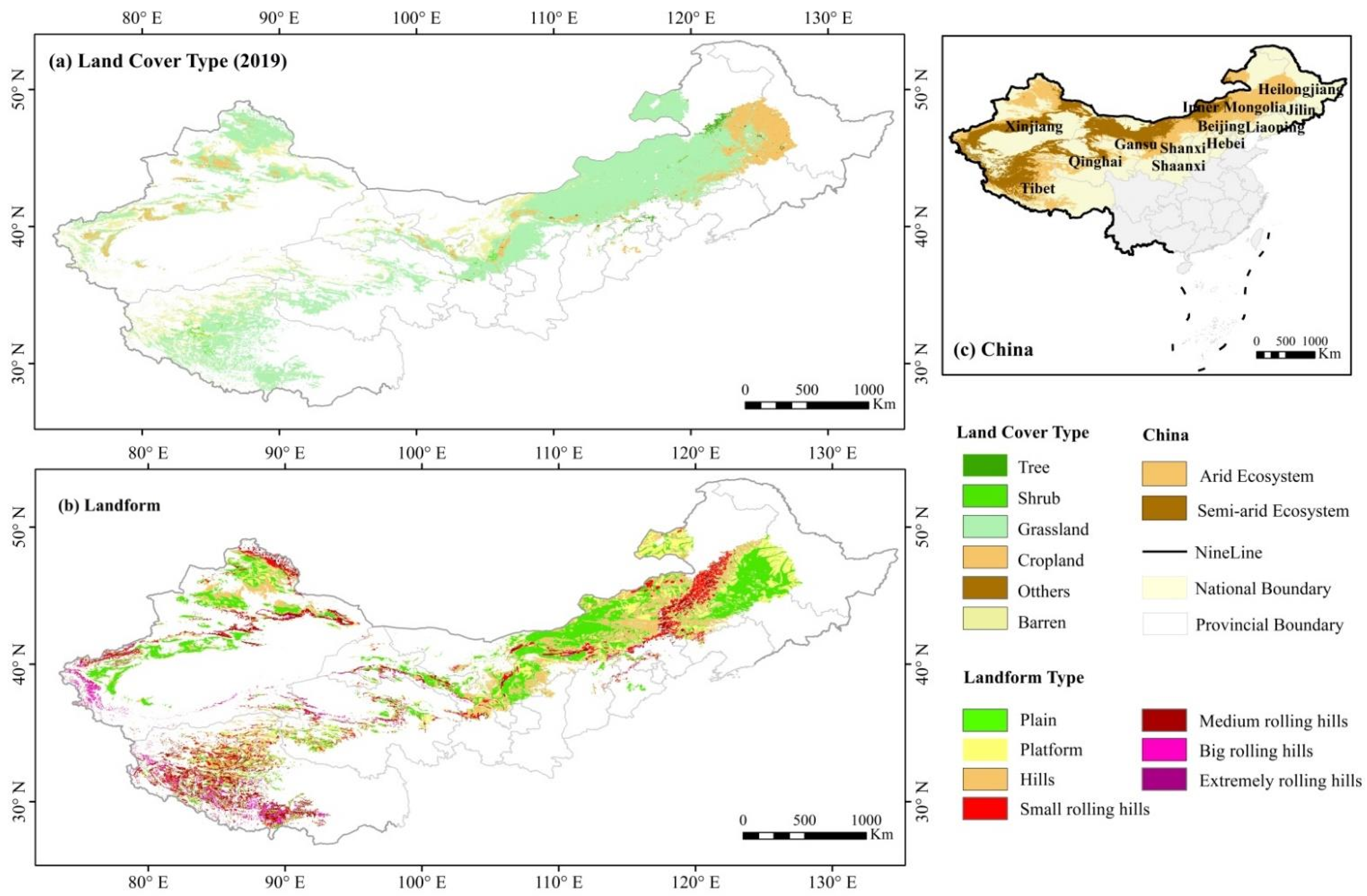
A multi-year average AI during 1951–2019 was used to define our study area. Since there is little vegetation in extremely arid regions (AI < 0.05), and precipitation may not be the main limiting factor for productivity in sub-humid regions (0.5 < AI < 0.65), making RUE an insufficient indicator of ecosystem functioning, only arid and semi-arid regions (0.05 ≤ AI < 0.5) were extracted to analyze the abrupt characteristics of RUE [38]. A monthly average NDVI less than 0.1 from March to November was used as the threshold to eliminate areas of sparse/absent vegetation [15]. ASARNC finally defined in this study covers an area of approximately 2.7 × 10⁶ km2, accounting for approximately 28.1% of the country’s land area (Figure 1). The annual precipitation decreases from east to west, ranging from approximately 400 mm to less than 100 mm. Furthermore, animal husbandry is the dominant industry in this region.
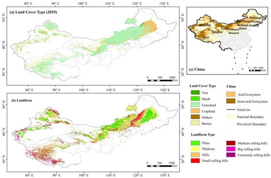
Figure 1.
The sketch map of the arid and semi-arid area of northern China: (a) land cover in 2019 (data from LAADS DAAC MOD12Q1); (b) landforms (data from Resource and Environment Science and Data Center, Chinese Academy of Sciences); (c) location in China.
2.2. Data Collection and Processing
2.2.1. MODIS Data
The MOD13A3 monthly composite NDVI from 2000 to 2019 and the MCD12Q1 yearly global land cover data during 2001–2019 were downloaded from the MODIS official website (https://ladsweb.modaps.eosdis.nasa.gov/ (accessed on 9 December 2021)). The MODIS Reprojection Tool (MRT) was used to perform band extraction, image mosaicking, and conversion from the sinusoidal projection to WGS84. Land cover types were reclassified into six classes, namely, cropland, grassland, shrubs, tree, barren, and others based on the plant functional types (PFT) classification scheme. In python3.8, the QA quality file was screened for the NDVI data, and the high-quality pixels of 00 were extracted to remove the interference of cloud, aerosol contamination, snow, and other factors on NDVI [49]. The resolution of the data is 0.00833 degrees per pixel, which is approximately 1 km × 1 km. The Earth trends modeler in the IDRISI TerrSet software (version 18.31) was used to fill the missing values of the images after the QA mask. The harmonic interpolation method was selected because it fully considered the phenological characteristics of surface vegetation and crops and ensured that the reconstructed time series NDVI data had statistical and ecological significance. According to the local crop rotation law of one crop per year in northern China, the number of harmonics was set to 1, and the value of 0 was used to fill the pixel values that were missing in a large area and could not be reconstructed by the harmonics so that the high-quality NDVI time-series data were generated [50].
2.2.2. Meteorological Data
The TerraClimate dataset [51] is a global high-resolution (1/24 degrees, similar to 4-km) monthly climate and climatic water balance dataset of the global terrestrial surfaces. Based on Google Earth engine (GEE), the precipitation (P) and potential evapotranspiration (PET) data of northern China from 1951 to 2019 were derived from the TerraClimate dataset. The gridded meteorological data used in this study were the monthly precipitation (P) dataset of China (1901–2020) with a spatial resolution of 0.008333 degrees (about 1 km × 1 km), downloaded from the National Earth System Science Data Center (http://www.geodata.cn/data/ (accessed on 27 December 2021)), which was verified by the observations in 496 independent meteorological stations. The monthly observed data from 692 meteorological stations from 1999 to 2019 were extracted from the daily value data set of China surface climate data (V3.0), provided by the National Meteorological Information Center (http://data.cma.cn/ (accessed on 25 April 2021)).
2.2.3. Other Data
Population density data were collected from NASA’s Socio-Economic Data and Application Center (https://doi.org/10.7927/H45Q4T5F (accessed on 22 December 2021)). The gridded GDP data and Chinese geomorphological data were obtained from the Resource and Environmental Science and Data Center, Chinese Academy of Sciences (https://www.resdc.cn/Default.aspx (accessed on 20 October 2021)). Both the population density and GDP data were taken every five years from 2000 to 2015 with a spatial resolution of 1 km. Additionally, the DEM data in China (2000) with the original resolution of 30 m were downloaded from the National Earth System Science Data Center, National Science and Technology Infrastructure of China (http://www.geodata.cn (accessed on 6 March 2022)).
The basic information concerning the data used in the study is listed in Table 1. The above data were subjected to coordinate system transformation, clipped, and resampled to be consistent with the scope of the study area.

Table 1.
The general information of the data used in our study.
2.3. Methods
2.3.1. Estimation of RUE
Prince et al. [52] observed that seasonal/annual cumulative NDVI could be used instead of NPP. Many studies have also demonstrated that changes in canopy optical thickness have no significant effect on NDVI variation in arid and semi-arid regions; therefore, NDVI can act as a proxy for ANPP, especially in the growing season [31,53,54]. In this study, the monthly MODIS NDVI (March to November) [55] were used to estimate RUE by the following equation:
where represents the NDVI value of the th month, and P represents the accumulated precipitation of the ith month.
2.3.2. Calculation of Drought Index
The standardized precipitation evapotranspiration index (SPEI) combines the sensitivity to evapotranspiration and the computational simplicity of the Palmer drought severity index (PDSI) with the multitemporal nature of the standardized precipitation index (SPI), making it ideal for exploring the impact of global warming on wet and dry regions [56,57,58]. According to China’s national meteorological drought standard, the SPEI is divided into nine categories, four drought, four wet, and one normal (Table 2) [59,60,61].
Table 2.
Categorization of drought and wet grade according to the SPEI.
Based on the monthly average temperature and accumulated precipitation of 692 meteorological stations in China from 1999 to 2019, we calculated the potential evapotranspiration (PET) by the Thornthwaite method and the monthly SPEI on a 12-month scale [59,62,63,64] using the SPEI package in R (vesion 4.1.1, https://cran.r-project.org/web/packages/SPEI/index.html (accessed on 23 February 2022)). Taking the DEM as a covariate, SPEI data were interpolated by the AUNSPLIN program. The gridded SPEI data were correlated with the global 0.5 degree 12-month SPEI data (https://spei.csic.es/spei_database/#map_name=spei01#map_position=1415 (accessed on 23 February 2022)) for validation, and 97.61% of the pixels passed the significance test (p < 0.05) (Supplementary Materials Figure S1).
2.3.3. BFAST Family Algorithms
BFAST family algorithms [65] enable the detection of breakpoints within earth observation time series, assuming that nonlinearity can be approximated by fitting a piecewise linear model [45,46]. The basic principle of the BFAST algorithm is to decompose the time series into seasonal, trend, and residual components, and choose a season-trend model to detect breakpoints in both trend and seasonal components. According to the number of breakpoints detected, there are the original BFAST model (detect all breakpoints in the time series) and BFAST01 model [15] (only detect 0 or 1 breakpoint in the time series) to provide. To improve speed and flexibility, BFAST Lite, derived from the original BFAST, can fit time series in a single step by using a multivariate piecewise linear regression [65]; it may overcome the problem of missing values in the RUE time series.
In our study, we mainly used the BFAST01 algorithm to detect the most influential changes in RUE, NDVI, and precipitation time series. With the BFAST01 model, the most influential break point with the largest amplitude in the time series can be detected [15]. For the time series obtained, a season-trend model is assumed with linear trend and harmonic season to fit the at time :
ere represents the intercept; denotes the slope of trend; represents the amplitudes; and are phases (i.e., season); f is the frequency of annual observations. In our study, f was 9 because we had nine observations in a year (March to November), and was the unobservable error term at time t. k = 3 means that three harmonic terms are employed to robustly detect abrupt changes in the time series.
The season-trend model can remove the stationary part (constant or periodically changing or slightly changing components) in the time series, and then focus on the residuals; that is, the time series is “detrended” and “deseasonalized” [66] after removing the fitted season-trend patterns. Equation (2) can be expressed as a standard linear regression model (see Chapter 3.3 in [67]), whose coefficients can be estimated and tested using ordinary least squares (OLS) techniques, and more details can see the reference [15]. In R 4.1.1, a time series was first computed by the above season-trend model to obtain a data frame with the response, seasonal terms, a trend term, (seasonal) autoregressive terms, and covariates, which could subsequently be fitted in a linear model. If there was a breakpoint that could minimize the segmented residual sum of squares, then the model with 1 breakpoint was selected to estimate the dating of the breakpoint. Finally, four tests for the null hypothesis of zero breaks were performed. Each test resulted in a decision for FALSE (no breaks) or TRUE (break(s)). The test decisions were then aggregated to a single decision (by using the function of any() in our research).
The detected break, if significant, could be considered a potential turning point in the ecosystem dynamics [17,24]. Then, the TP type could be determined based on linear trend fitting before and after the detected TP, and the regions where no TPs were detected could be divided into two monotonic types. We finally identified eight trend types based on De Jong’s [15] classification method, that is, two types of no TPs and six TP types (Table 3 and Figure S2). Additionally, the linear trend fitting before and after the detected TP could be tested using OLS techniques. There are four test results according to the significance of each segment, which are shown in Table 4.
Table 3.
Trend types of ecosystem functioning based on rain use efficiency.
Table 4.
Significance of both segments before and after the detected TP.
In addition, the BFAST algorithm was used to analyze the SPEI time series to detect its maximum abrupt amplitude. The natural breakpoint method in ArcGIS was applied to reclassify the break amplitude. According to the meaning of the SPEI, we assigned a 0 value as the threshold to distinguish whether the break direction of the SPEI was positive (wet) or negative (drought).
All the BFAST family algorithms used in this study were carried out in R 4.1.1, and the parameter settings are illustrated in Table S1.
2.3.4. Determining the Turning Point Occurrence Index (TPOI)
The TP confidence level was used to identify the areas with high/low TP confidence. Different significance test methods identified different TPs. To avoid the issue of TPs being affected by the limitations of an individual significance test, we adopted four tests (BIC, OLS-MOSUM, SupF, and SupLM) in BFAST01 to develop the TPOI proposed by Bernardino et al. [24]. Provided that any of the significance tests passed (p < 0.1), the pixel was considered to have undergone a TP. Combining the test result of the BFAST Lite algorithm with those of BFAST01, the number of TPs in each pixel was obtained using spatial overlay analysis in ArcGIS, from which the TPOI was then calculated. In this case, if all four test methods and the BFAST Lite algorithm detected the TPs in a pixel, the TPOI of the pixel was 1. If only one test detected the TPs, then the TPOI was 0.2, and so on, thus obtaining the map of the TPOI during 2000–2019.
2.3.5. Correspondence Analysis (CA) of SPEI Grades and TP Types
CA is a data visualization method suitable for two-dimensional contingency table data. The results can reveal the correlation between two categorical variables and the differences or similarities of the same categorical variable [68,69]. Therefore, we employed CA to explore the impact of drought on TP types in the EF. The drying or wetting conditions corresponding to the occurrence of TPs were analyzed based on the SPEI. The closer one RUE type was to a certain SPEI grade, the greater the consistency between them. Due to the potential lagging effects, the SPEI three months before TPs were also considered to analyze the duration of continuous drought or wetness [58]. According to the number of drought or wet occurrenced in these four months, the duration was marked as 0–4 months.
2.3.6. Frequency of Land Cover Change
Here, we focus on the frequency of changes rather than the type of land cover change. For example, if the land cover type was converted between grassland, cropland, grassland, and cropland in 19 years, then we considered the times of land-use change in this pixel to be 3, and so forth.
3. Results
3.1. Turning Points in Ecosystem Functioning Based on RUE
3.1.1. Spatial Distribution of TPOI
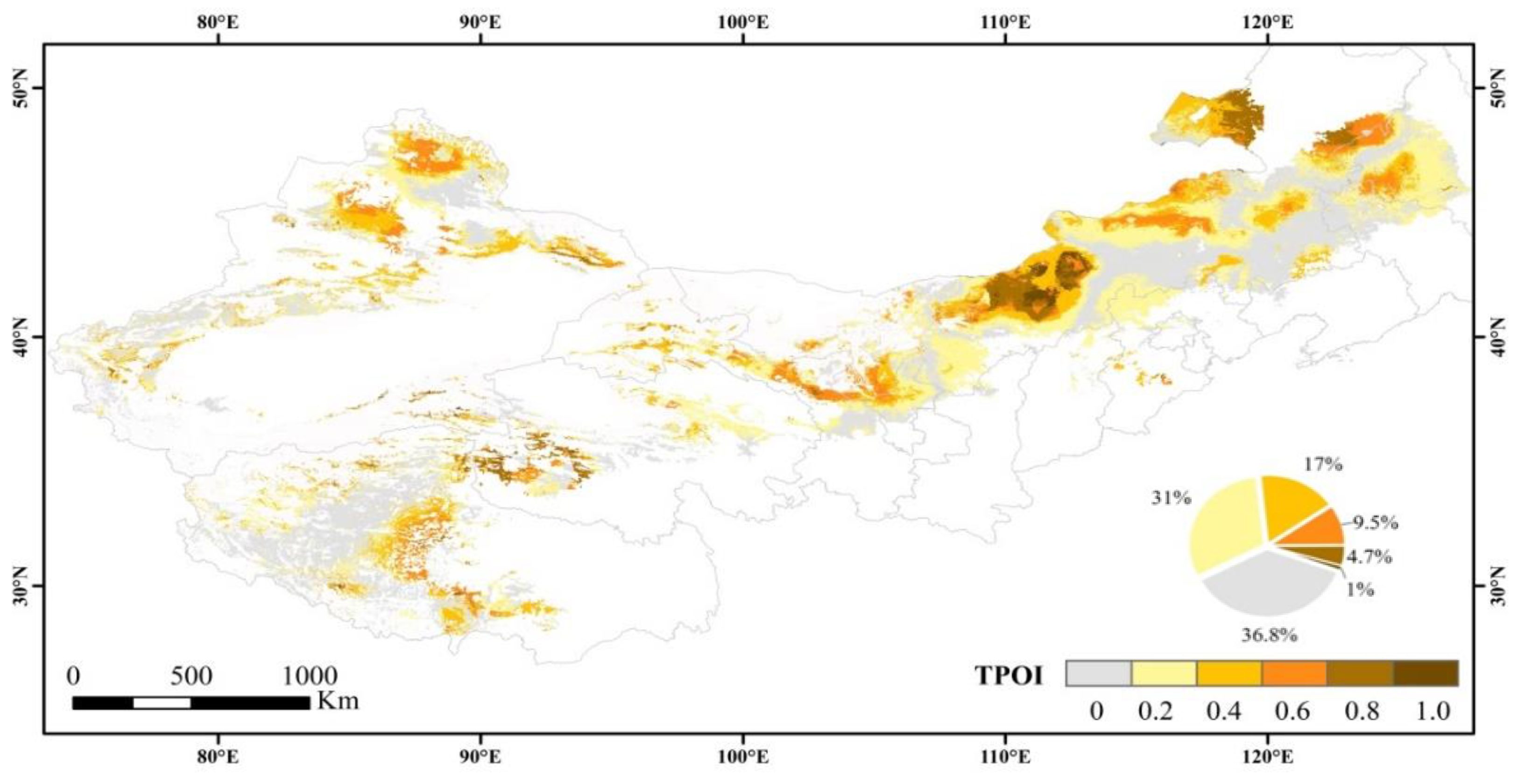
As shown in Figure 2, the EF in the ASARNC has significantly changed in the past 20 years. TPs were detected in a total of 63.2% of the study area (approximately 1.71 × 10⁶ km2), of which 50.92% passed two or more significance tests. A high TPOI (TPOI > 0.6) accounted for 15.2% of the total TPs. Of these TPs with a high TPOI, 5.7% were extremely high (TPOI > 0.8) and located at the junction of the northwestern Songnen Plain, western Hulunbuir, and central Inner Mongolia.
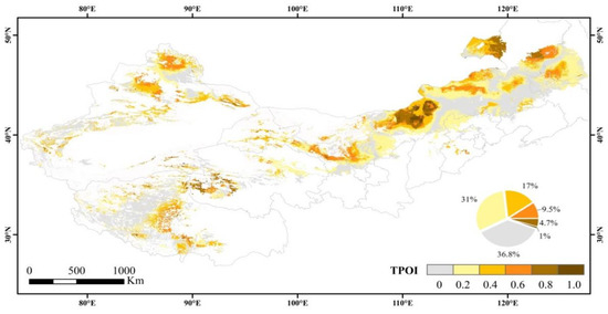
Figure 2.
TPOI of ecosystem function in arid and semi-arid regions of northern China (p < 0.1, of which 89.22% of the pixels have passed the p < 0.05).
3.1.2. Trend Types of EF
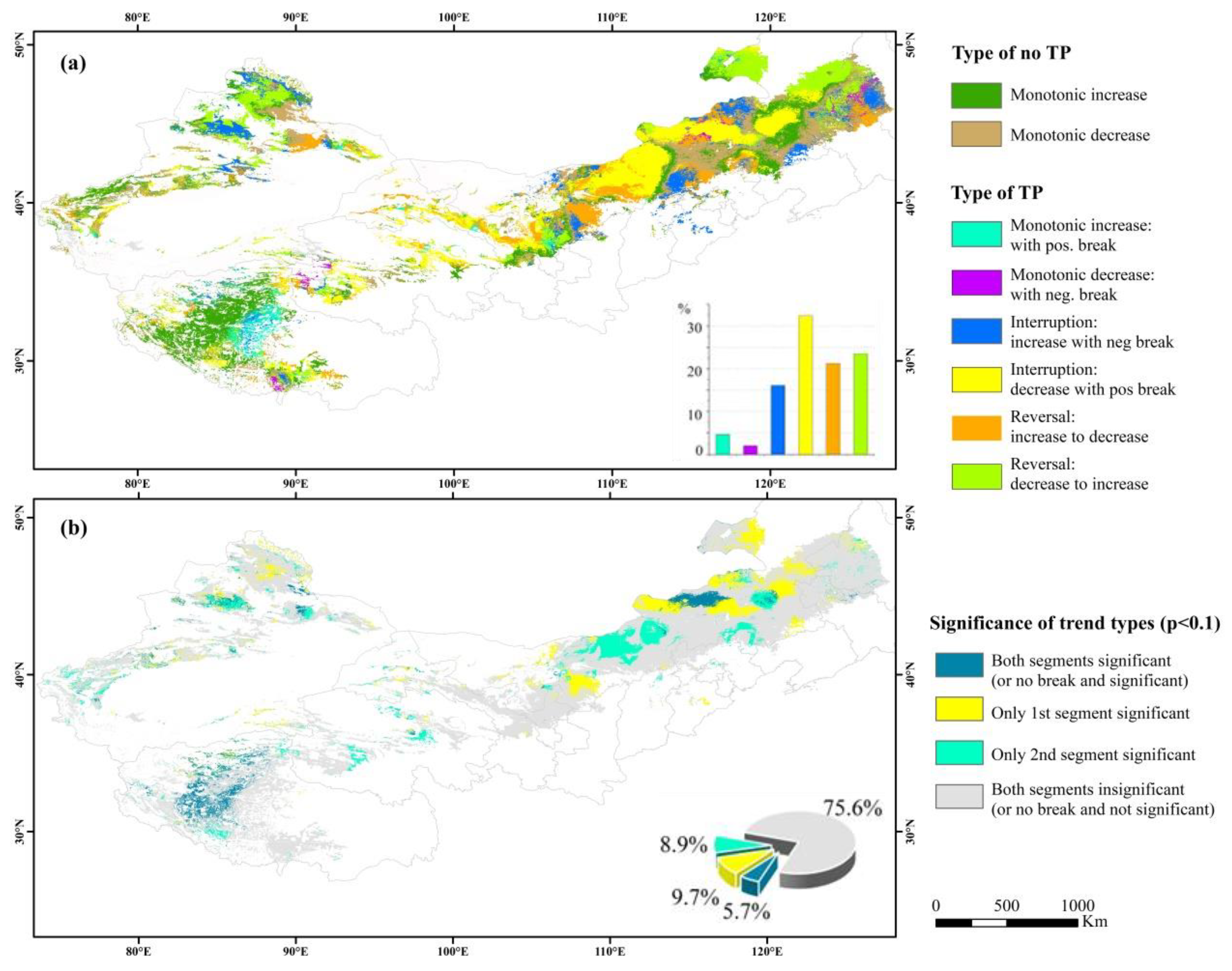
From 2000 to 2019, Type 6 (Interruption: decrease with positive break) was the dominant TP type, mainly observed in central and eastern Inner Mongolia, central Gansu, and western Ningxia (Figure 3a). There was a clear correlation between the spatial distribution of Type 5 (Interruption: increase with negative break) and Type 7 (Reversal: increase to decrease), implying that these areas might have encountered the same external interference. In some areas, the anti-interference was relatively strong, so the RUE could return to the previous state after a short drop. Conversely, RUE decreased in other areas due to the weaker ecosystem resilience. There were very few Type 3 (Monotonic increase with positive break) and Type 4 (Monotonic decrease with negative break) pixels detected. We speculate that these two types might be identified as Type 1 (Monotonic increase) and Type 2 (Monotonic decrease) by the algorithm due to the relatively small magnitude of breaks in the study area. Meanwhile, the significance of trend types was analyzed. According to Figure 3b, 91.2% of the pixels with monotonic trend were found to be insignificant, indicating that the change trend of RUE in these areas was not obvious and the ecosystem functioning was stable. For 66.5% of the pixels in TP types, changes in trend both before and after TP were not significant. External interference caused RUE in these areas to rise or fall significantly, causing the ecosystem to turn to a new and stable functional state.

Figure 3.
Distribution of trend types of EF detected based on RUE (a) and the significance test of TP types (b).
3.1.3. Timing of TPs
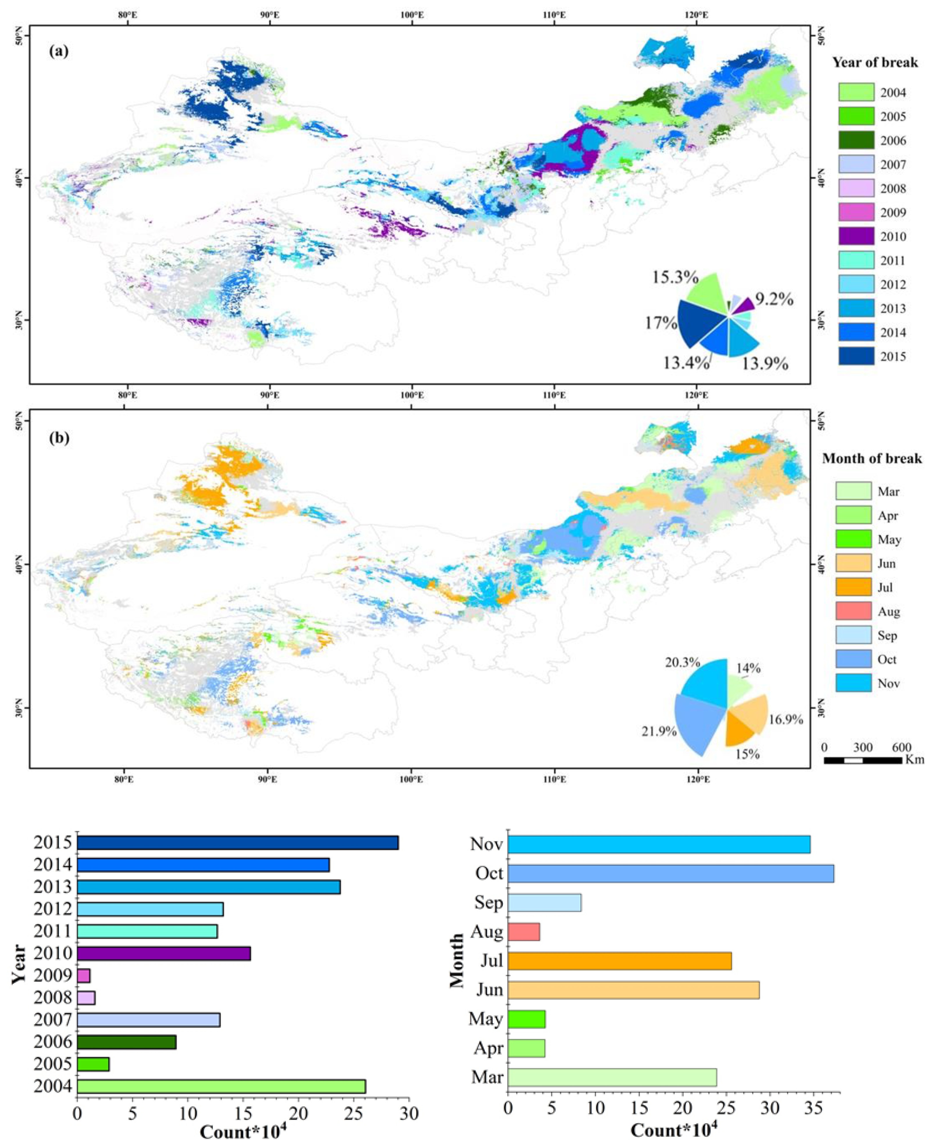
To more intuitively display the year and month of TPs (such as June 2007, November 2007, and June 2008) and better understand the year and month characteristics of TPs in the study area, the timings of TPs were classified by year (Figure 4a) and month (Figure 4b). For example, the TPs that occurred in June 2007 and November 2007 were both expressed as 2007 by year, and the TPs that occurred in June 2008 and June 2007 were both expressed as June by month. Combined with Figure 4a,b, the specific year and month of the TPs in a region were determined. In the past 20 years, there were several years in which the break in EF in the study area was overwhelmingly pronounced, such as 2004, 2013, 2014, and 2015, accounting for 59.6% of the total TPs (Figure 4a). In 2008 and 2009, there were the lowest numbers of TPs, indicating that the EF was relatively stable. Most TPs occurred in October, followed by November (Figure 4b). Additionally, June and July also contained a greater number of TPs. Only 14% of the TPs were detected in March.
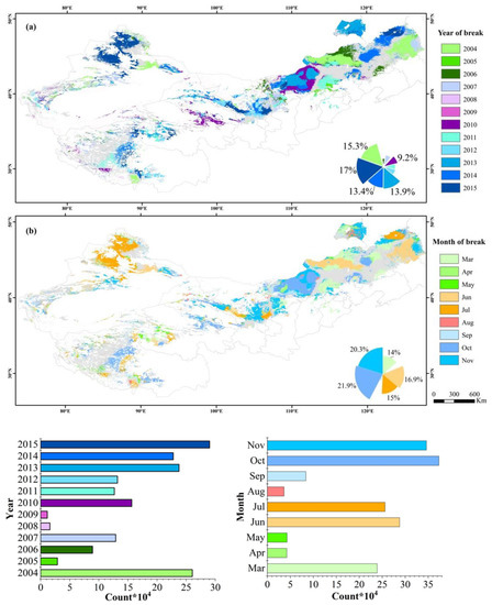
Figure 4.
Timing of TPs in EF (p < 0.1): (a) year; (b) month.
3.2. Effects of Drought on TPs in Ecosystem Functioning
3.2.1. TPs of SPEI
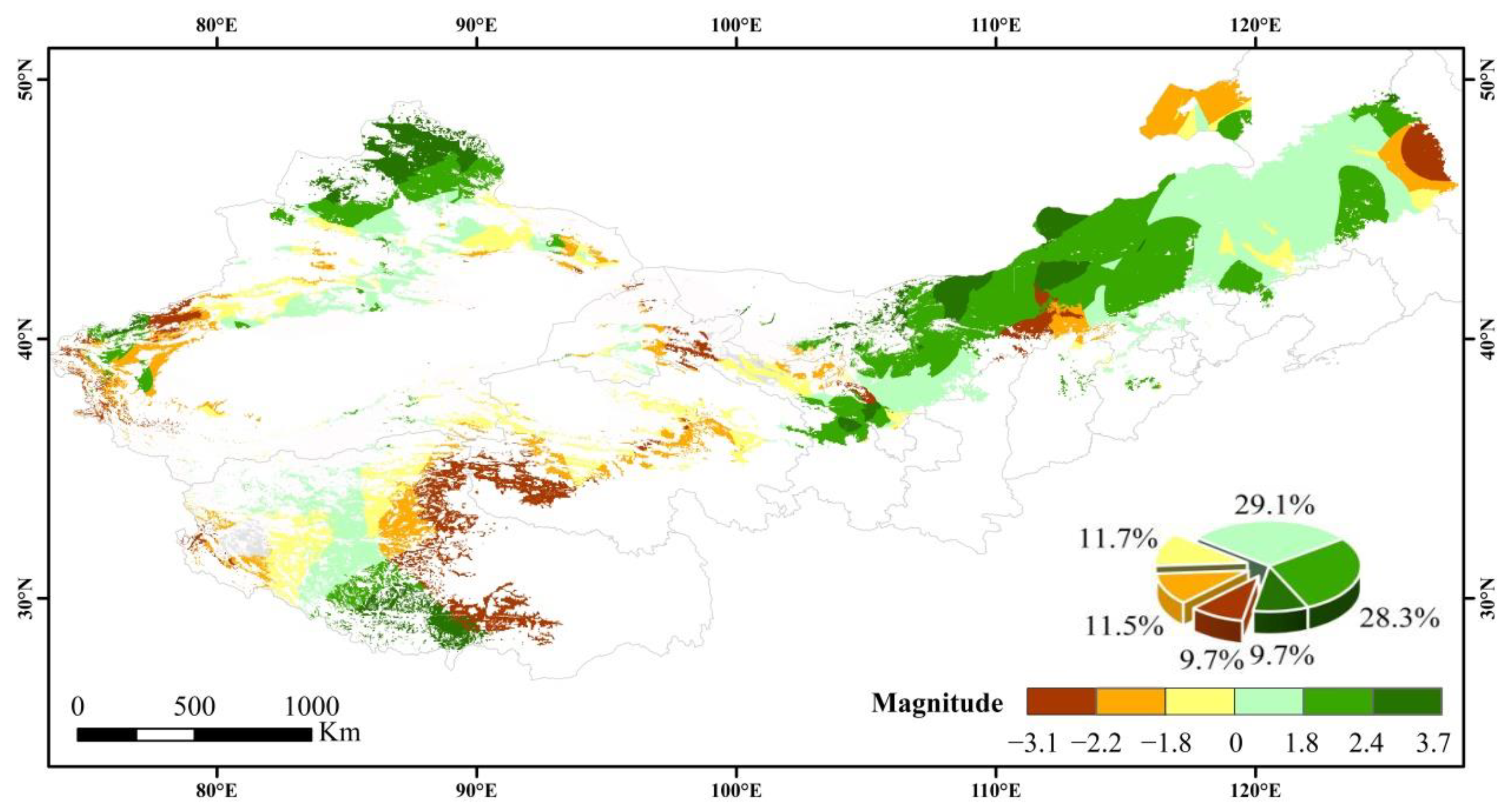
During 2000–2019, 67.3% of the largest magnitudes of break in the SPEI were positive, showing a wetting trend. However, the pixels with negative changes accounted for approximately 32.7% of the study area, indicating that these areas were strongly affected by drought (Figure 5).

Figure 5.
The largest magnitude of break in the SPEI from 2000 to 2019 (p < 0.05).
3.2.2. CA of Drought and TP Types
The relationships between drought/wet status when a TP occurred and the duration of drought/wet before the TP occurrence and the TP types were analyzed. From Figure 6, 22.2% of the pixels detected drought when TPs occurred, which mainly occurred in the Xilingol League, Inner Mongolia in March 2006, northern Xinjiang in July 2015, and southwestern Heilongjiang in November 2007, while the rest of the pixels were in a drought-free or humid state. Namely, only 22.2% of the TPs could be explained by drought.
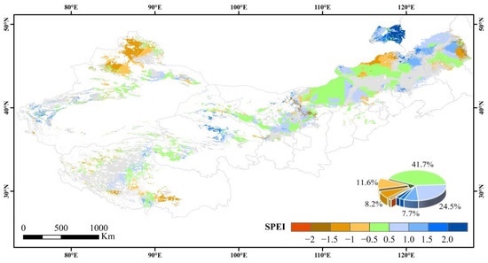
Figure 6.
Distribution of SPEI grades when TPs occurred.
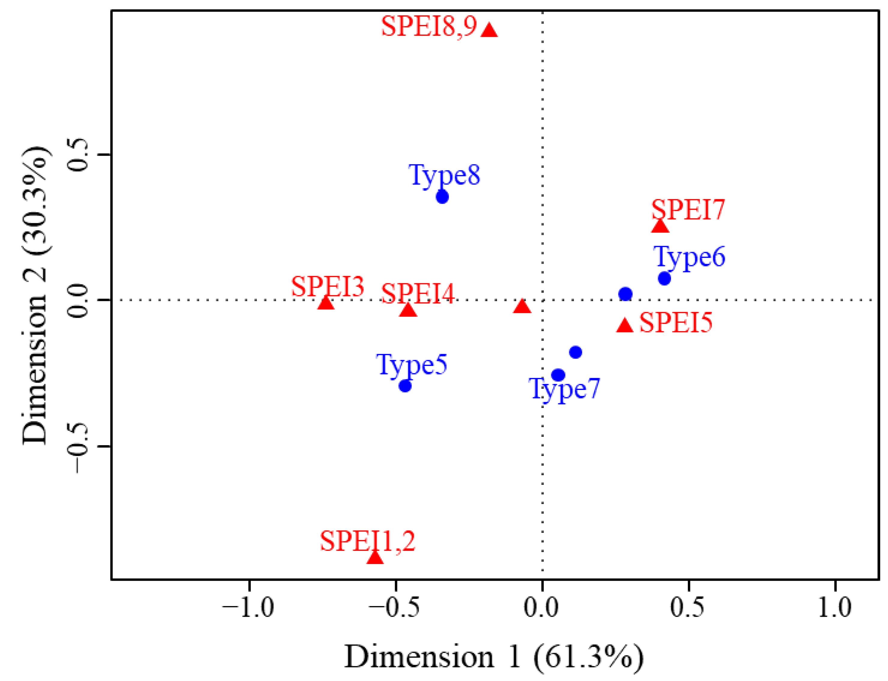
The CA result shows that the first two dimensions together explained 91.69% of the deviation from independence between the SPEI level and the TP type, indicating that there was a strong correlation between them (Figure 7). Furthermore, the CA method distinguished drought and drought-free types and different SPEI categories well. From Figure 7, Type 8 (Reversal: decrease to increase) was the closest type to SPEI 8 (Severe wet) and SPEI 9 (Extreme wet). This result might be due to the sudden increase in precipitation in the extremely humid climates, which promoted vegetation growth and increased the net primary productivity, thereby improving the rain use efficiency. In contrast, the nearest TP type to SPEI 1 (Extreme drought) and SPEI 2 (Severe drought) was Type 5 (Interruption: increase with negative break). This might be attributed to the death of vegetation caused by drought, causing the RUE to decrease suddenly. After drought, the vegetation productivity slowly recovered, and the RUE increased accordingly. Drought was not the main cause of Type 7 (Reversal: increase to decrease), as seen from the positional relationship between Type 7 (Reversal: increase to decrease) and SPEI 5 (Normal). Similarly, Type 6 (Interruption: decrease with positive break) had little correlation with drought.
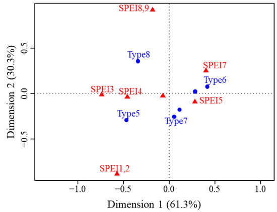
Figure 7.
Correspondence analysis between SPEI grades when TPs occurred and TP types (Only the categories that contribute more than 70% to the coordinate axis are showed in the figure. As the pixels of the detected SPEI 1, SPEI 2 and SPEI 8, SPEI 9 were much less than those of other types, they were combined to express).
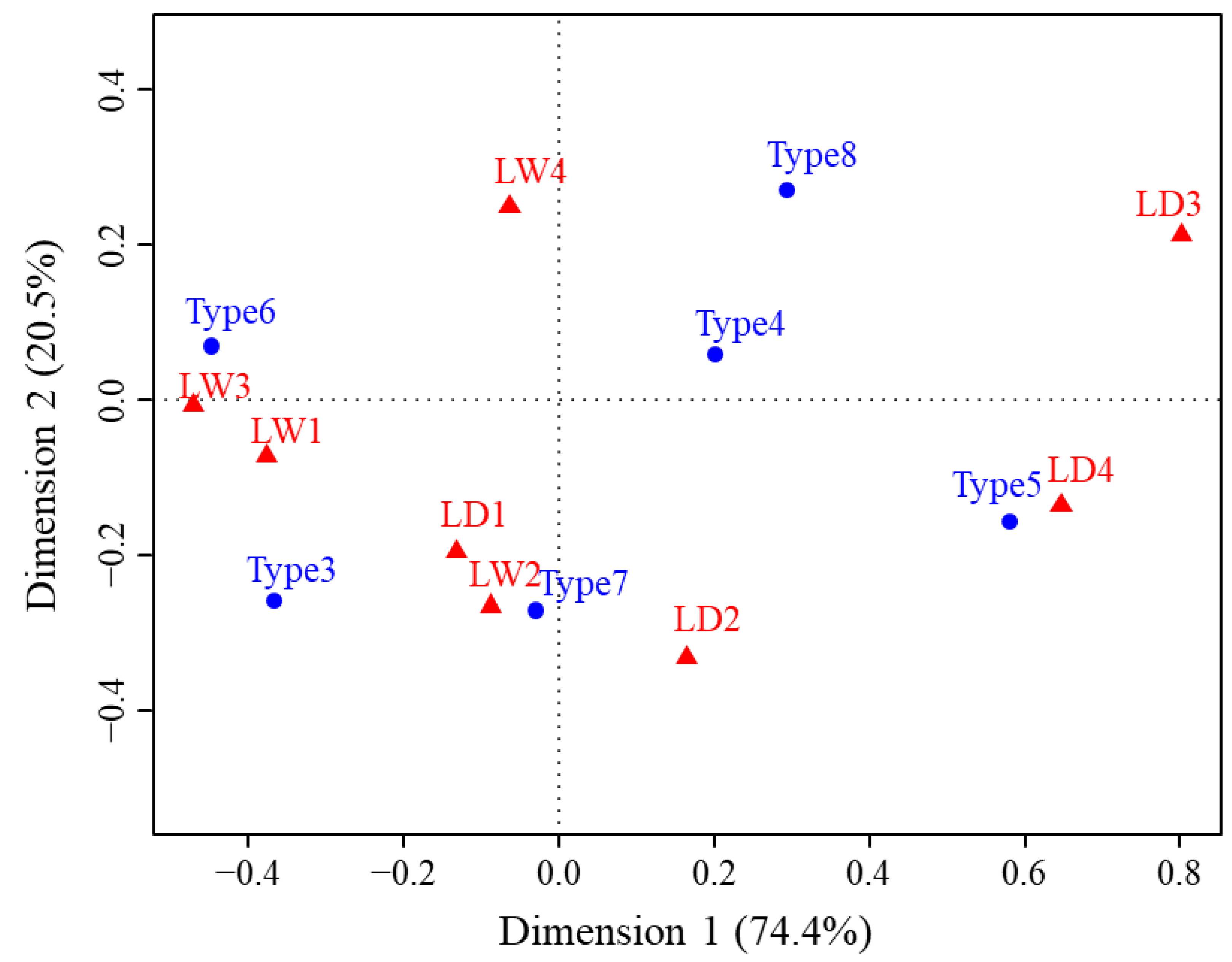
The distribution of continuous drought/wetness detected in the same month and three months preceding the TPs is shown in Figure 8. The drought/wetness continuity was essentially consistent with the dry/humid state when the TP occurred, suggesting that the 12-month SPEI could reflect the drought/humidity state in the study area. According to the CA of the TP type and the duration of drought/wetness (Figure 9), the first two dimensions explained 94.9% of the deviation from independence, indicating that the lasting dry/humid state before the TP had a stronger correlation with the TP type. LD2, LD4, and LD3 could be well separated from LW1, LW2, LW3, and LW4 by CA analysis (Figure 9). Type 4 (Monotonic decrease with negative break), Type 5 (Interruption: increase with negative break), and Type 8 (Reversal: decrease to increase) were associated with lasting drought, while Type 3 (Monotonic increase with positive break), Type 6 (Interruption: decrease with positive break), and Type 7 (Reversal: increase to decrease) were more consistent with the condition of continuous wetness; in other words, they had very little linkage to drought.
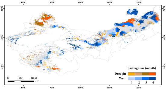
Figure 8.
Distribution of lasting drought/wetness detected in the same month and three months preceding the TPs.
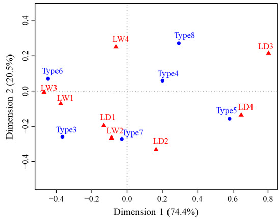
Figure 9.
Consistency of lasting drought/wet and TP types (LD1, 2, 3, and 4 represent the SPEI’s lasting drought (LD) for 1–4 months, and LW1, 2, 3, and 4 represent the SPEI’s lasting wetness (LW) for 1–4 months, respectively).
3.3. The Linkage between the Frequency of Land Cover Change and TPOI
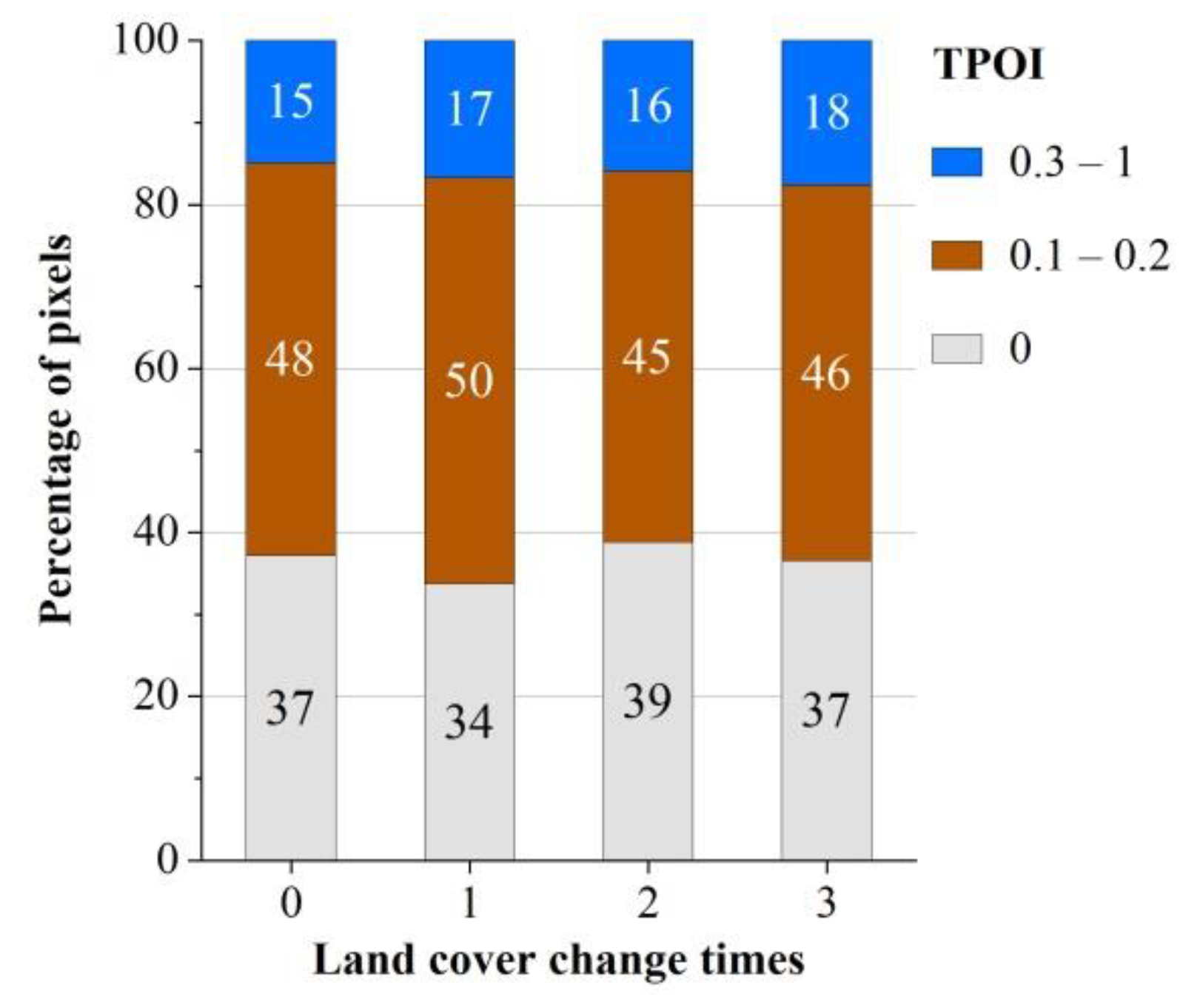
From 2000 to 2019, 13.4% of the land cover pixels changed (Figure 10). Most of the land-use types changed at least three times, and grassland was the most frequently changed type.
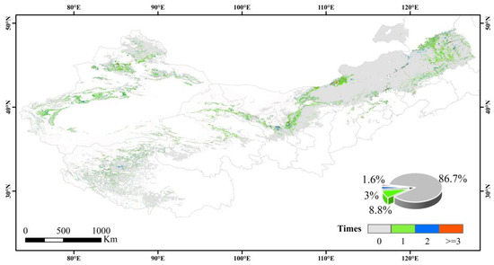
Figure 10.
Number of land cover changes.
A high TPOI (TPOI ≥ 0.6) is more likely to be found in areas with more frequent land changes (Figure 11); however, the proportion of TPOI for different frequencies of land cover change has little overall difference.
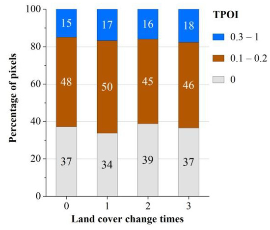
Figure 11.
Distribution of the percentage of TPOI for different frequency of land cover change.
3.4. The Impact of Population Density and GDP Changes on the TPs
To analyze the relationship with the TPs of EF, the population density was classified into three classes using the equivalence method [24], while GDP was divided into three categories at equal intervals (Table 5). We calculated the differences between population density and GDP for every 5-year interval, and the results showed that both the population density and GDP have changed greatly in some areas over the past 20 years (Figure S3).
Table 5.
Classification of population density and GDP.
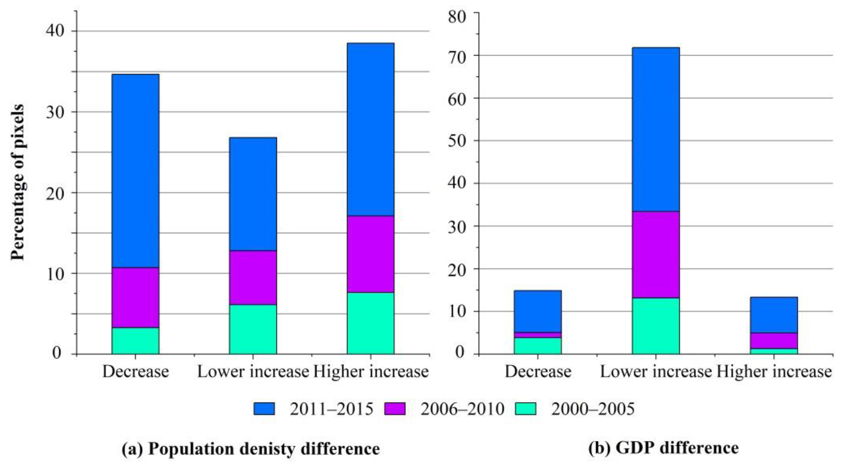
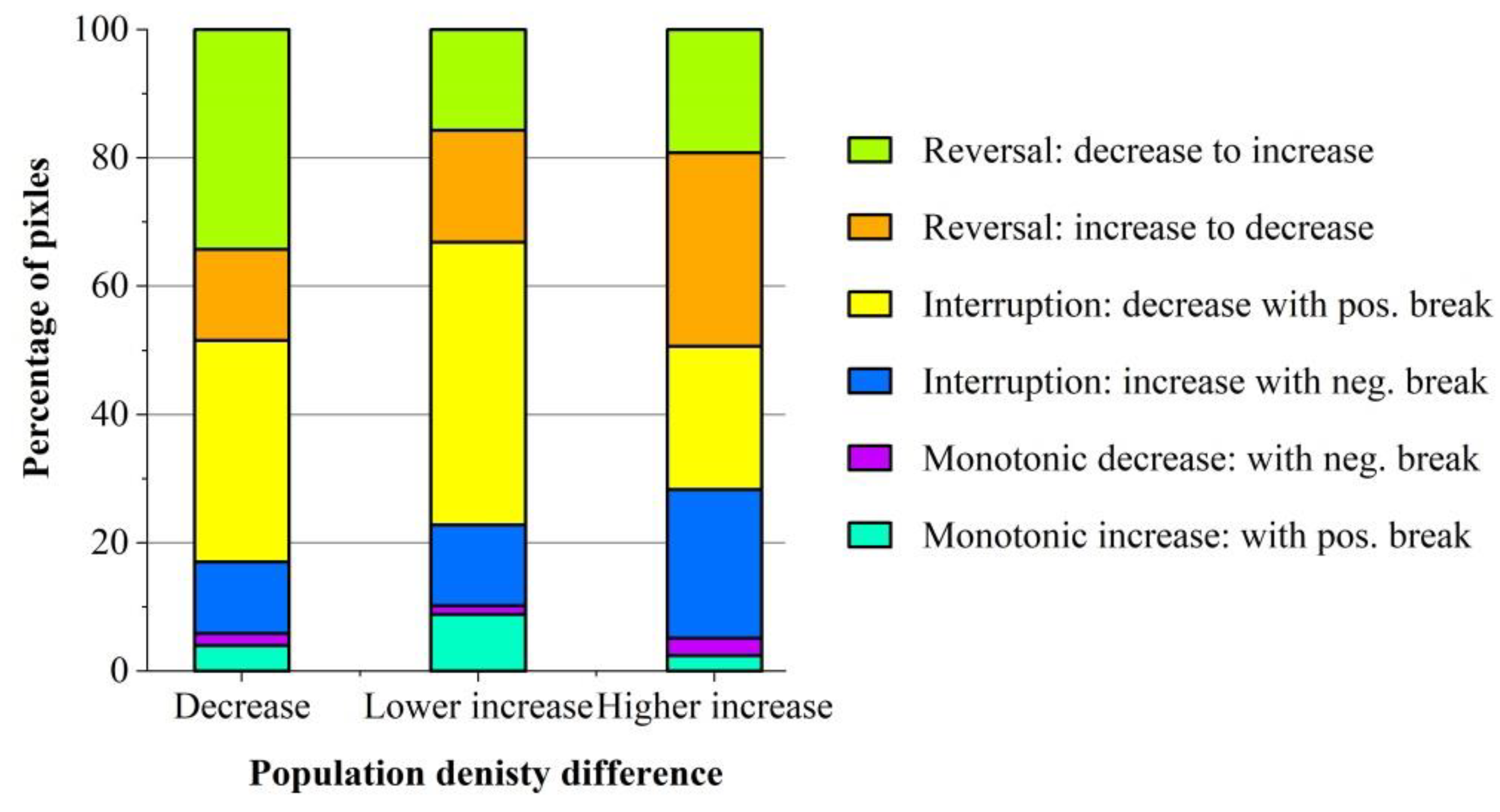
During 2000–2015, 65.33% of the TPs occurred in areas with increasing population density, of which 38.52% were found in rapidly growing areas. On the other hand, there were also many TPs in areas with reduced population density, accounting for 34.67% of the total TPs (Figure 12a). TPs were concentrated in areas of slow GDP growth, while fewer TPs were found in regions with declining GDP. Especially from 2005 to 2010, 95.36% of the TPs were found in places with GDP growth (Figure 12b). According to Figure 13, Type 8 (Reversal: decrease to increase) accounted for a high proportion of areas with decreased population density, while Types 7 (Reversal: increase to decrease) and Type 5 (Interruption: increase with negative break) occupied more areas with increased population density. Type 6 (Interruption: decrease with positive break) and Type 3 (Monotonic increase with positive break) accounted for higher proportions in locations where population density increased more slowly.

Figure 12.
Distribution of the percentage of TPs under changes in population density (a) and GDP (b) (every five years).

Figure 13.
Distribution of the percentage of TP types under different population density changes.
4. Discussion
4.1. Relationship between Change Trends of Precipitation, NDVI, and RUE
To understand the whole-view on the changes in corresponding variables in the study area, the temporal profiles for the whole regional mean P, NDVI, RUE, and SPEI were presented. As shown in Figures S4 and S5, NDVI and precipitation in the study area showed an overall increasing trend from 2000 to 2019, making the RUE trend almost stable, which was consistent with the results obtained by using the BFAST method (In Figure 3b, 75.6% of the pixels in the study area had no significant change trend).
The trend analysis of NDVI and precipitation time series based on Theil-Sen [70,71] and the BFAST01 method helped to identify their underlying effects on RUE variations for the period of 2000–2019. The abrupt change in precipitation mainly occurred in the eastern part of the study area, namely, southwestern Heilongjiang, the west of Jilin, Xingan league, and Tongliao City of Inner Mongolia (Figure S7). Precipitation in the central and eastern part of the study area showed a positive trend, among which the central Inner Mongolia (i.e., the west of Xilingol League and the north of Ulanqab) experienced significant increase in precipitation (Figure S6a). In southwestern Heilongjiang and western Jilin, a significant increase trend of precipitation was found before 2015 (Figures S7 and S8). However, a sudden decrease in precipitation in these areas was detected around 2015, resulting in an increase in RUE in southeastern Hulunbuir, northwestern Chifeng, and Xingan league in Inner Mongolia during this period (Figure S6b). The decreasing trend of precipitation was detected only in the northern part of Xinjiang, where the precipitation suddenly increased in 2015, leading to the abrupt decrease in RUE accordingly (Figure S6c). In addition, we found that the abrupt change in precipitation mainly occurred in summer, followed by spring and autumn. This partially reflects the importance of changes in summer and spring precipitation for ecosystem function variations in ASARNC.
According to Figure S6, 86.03% of NDVI pixels in the study area suffered abrupt changes in the past 20 years (p < 0.1), and the overall trend of NDVI detected by BFAST01 was in good agreement with the results of the Theil-Sen trend analysis (Figure S11, p < 0.05). Spatially, NDVI shows a significant trend of increase on the whole, and the results of BFAST01 provide more information about NDVI abrupt changes. In the northeast of the study area and Xinjiang, the abrupt changes were mainly positive (Figure S6d), while NDVI values in the middle of the study area, Qinghai and Tibet were affected by negative interference (Figure S6e). In terms of occurrence time, the break years of NDVI were relatively scattered, slightly more in 2015 (Figure S10). The break months of NDVI were mainly distributed in summer (taking up 50.5% of the total) and spring (32.8%), which was consistent with the seasonal distribution characteristics of precipitation, implying that NDVI is easily affected by external factors in summer.
Precipitation in western Tibet experienced a significant decrease, while its NDVI had a significant upward trend (Figures S11 and S12). Therefore, the RUE in central and western Tibet (p < 0.1) showed a significant increase in trend (Figure S6e). In eastern Inner Mongolia, especially in the Xing’an League and Tongliao areas, both the NDVI and precipitation showed a significant upward trend, making the RUE in these regions stable (Figures S13 and S6f). Although the abrupt characteristics of NDVI or precipitation in some regions might determine the break features of RUE, TPs in RUE in most area of ASARNC attributed to the combined effects of the above two variables, forming different TP types associated with the differences of regional ecological environment. The TPs that only occurred in NDVI or precipitation may not cause the abrupt change in RUE.
The spatial distribution of the monotonic RUE increase was similar to that of the monotonic decrease; 13.7% of the monotonic increases and 16% of the monotonic decreases were stable. Stable pixels mostly occurred at the junction of the above two types and were distributed in strips near the mountains. In most of these areas, NDVI and precipitation showed a synchronous increasing and decreasing trend; thus, the stable RUE might be due to limited human intervention and a relatively smaller human footprint. Meanwhile, the detected monotonic changes were mostly insignificant, indicating that changes in RUE were characterized by volatility and stability in these regions, that is, EF was stable (Figure S13).
4.2. Abrupt Change Characteristics of Ecosystem Functioning
We detected TPs by using monthly RUE data so that the changes in EF in the ASARNC at a finer spatiotemporal scale could be explored. From 2000 to 2019, 63.2% of the pixels were classified as TPs in the study area, and 15.2% of the pixels had a high TPOI (TPOI > 0.6). Among the eight trend types, Type 6 (Interruption: decrease with positive break) was the most common, accounting for 20.4% of the total pixels and 32.4% of the TPs.
The detected TPs were not only the result of the deterioration of EF caused by factors such as drought but also might be attributed to the improvement of the ecological environment. Figure 5 shows that 67.1% of the most significant TPs in SPEI were positive, i.e., breaks toward climate wetting, which was similar to previous studies [72]. Negative changes were detected only in northwest China, which was also demonstrated in the study presented by Miao et al. [73]. According to the types detected by BFAST01 (Figure S14), the SPEI in the eastern part of the study area showed a significantly positive increase (p < 0.1), but negative interference also occurred. SPEI in the northwest mainly showed negative growth, during which positive TPs occurred. The overall trend detected in this study was consistent with the future changes in China’s drylands estimated by Miao et al. [73]. The study area was much more affected by humid climate than drought in the past 20 years. We found that the precipitation in most areas showed an insignificant increasing trend (Figure S12), similar to the findings of Miao et al. [73] and Liang et al. [74], while the NDVI increased significantly for 57.8% of the pixels (Figure S11). To a certain extent, the overall ecological environment in the study area is improving, which may be related to the various ecological restoration projects that have begun since approximately 2000 [75,76,77], which have enhanced greening trends. On the other hand, 59.4% of the detected TPs in this study occurred after 2010. Related studies similarly found that the overall warming and wetting climate in northwest China since 2010 had a positive impact on vegetation health [78,79,80,81]. Additionally, afforestation, grazing prohibition, and other ecological restoration projects were regarded as the major drivers of vegetation restoration [82,83]. The lowest number of TPs were detected between 2008 and 2009, and some studies found that there was no significant climate change in northern China during this period [84].
4.3. Influencing Factors of TPs in Ecosystem Functioning
The occurrence time (i.e., year and month) and types of the TPs may indicate a transformation in the underlying mechanism of ecosystem functions. During 2000–2019, persistent drought events were detected in 16.56% of the TPs in the study area (Figure 8), which were mainly distributed in the Xilingol League of Inner Mongolia, northern Xinjiang, and southwestern Heilongjiang. Among these, we detected drought events around the TPs on March 2006 and November 2007 in the eastern part of Xilingol League, an interval coinciding with the driest year in Xilingol, 2007 [62,85]. Zhao et al. [86] also found that the aboveground biomass of the Xilingol steppe fluctuated greatly from 2007 to 2010, and the lowest value was observed in 2007. The TP types in the Xilingol League showed obvious spatial differences, and Type 5 (Interruption: increase with negative break) and Type 7 (Reversal: increase to decrease) dominated in the central and eastern parts, respectively. The same drought event had different effects on EF, which might be related to the distribution of grassland coverage increasing from west to east [86]. The resistance of grassland ecosystems with different coverage varied, resulting in different effects on the change in the ecosystem after interference [17]. High-coverage grassland ecosystems with a strong ability against disturbances might restore their functions after drought; thus, the TP type was mainly Type 5 (Interruption: increase with negative break). In contrast, the anti-disturbance ability of low-coverage grassland ecosystems was weak, and drought might cause the rising trend of RUE to begin to fall.
Similarly, drought-dominated TPs were also detected in Suihua city of Heilongjiang Province in November 2007, causing RUE to undergo a negative break (Figure S6d). It was verified that Suihua experienced a 50-year drought event in the summer of 2007 [87], which caused a decline in RUE. The TPs detected in northern Xinjiang were mainly in July 2015, when that region experienced a lasting drought event. There are several TP types, and the RUE trends before and after the TPs differ, but they have in common the fact that the TPs were negative, which can be considered the effect of drought.
The linkage between TPs and drought was weak in the remaining areas. For instance, no drought events were detected at the TPs in the western part of Hulunbuir, Inner Mongolia, in November 2013. We diagnosed the continuous humid events, which were consistent with the results of Zhang et al. [88]. The TP type was Type 8 (Reversal: decrease to increase), and RUE showed a significant decreasing trend before the break but did not increase significantly after break (Figure S6g). This may be related to the fact that vegetation in Hulunbuir generally declined before 2010 and slowly increased after 2010 [89].
Therefore, persistent drought was not the main factor causing most of the TPs in the study area over the past 20 years. This might be due to the regularity and stability of RUE, i.e., the surrogate index of EF used in this paper. Drought events had a limited impact on RUE. In contrast, we detected persistently humid states in most of the TPs, which suggested that a humid climate affected the EF in the ASARNC to some extent, which was similar to the results of Na [90]. In addition, the SPEI was in a neutral condition when the break was detected in the western Xilingol League, indicating that the TPs might be attributable to human activities and have nothing to do with drought or wet events. Spatially, the SPEI values were within the normal range when the TPs in this study occurred mainly in southwestern East Ujumqin Banner, the middle of Abaga Banner, and northern Xilinhot. This pattern was similar to the spatial distribution of higher grazing pressure found in previous studies [91,92,93].
Land cover is another way in which human activities promote changes in EF [17]. Our results show that the frequency of land cover changes in this study area was not the main factor causing the TPs of EF. This may be due to the absolute dominance of grassland and the limited number of times that the land cover changed. Population density is closely related to changes in ecosystems. The TPs were not highly concentrated where the population density was increasing in our study, which was associated with the population decline in the study area over the past 20 years [94]. Overall, there is a definite correlation between population density changes and the TP type. In areas with reduced population pressure, the trend of EF following TPs was upward, while more negative TPs were detected in areas with a relatively increased population and where the EF trend was downward.
4.4. Applicability of the BFAST Family Algorithms for Detecting Changes in Ecosystem Functioning
In this study, the TPs detected from the time series RUE ranged from 40 to 140, corresponding to the years 2004 to 2015. It can be seen that the BFAST algorithm could not detect breakpoints at the beginning and end of the time series (i.e., the first 40 and the last 40 time points). The limitations of this algorithm itself might also reduce the thoroughness of our TP detection while ignoring the information on ecosystem function changes before 2004 and after 2015. Almost all pixels with TPOI values greater than 0.6 were detected by the BFAST Lite algorithm, implying its high reliability in detecting TPs in the study area. Moreover, the TPOI detected by BIC was almost 100%, while the two testing methods with the greatest disagreement were SupLM and OLS-MOSUM. SupLM detected the most TPs, accounting for 56.46% of the total pixels, while OLS-MOSUM detected the fewest TPs, accounting for only 4.74% (Figure S15).
Some previous studies proved that the 12-month SPEI could better characterize the regional dry and wet state, but Tong et al. found that the Xilingol grassland had a stronger response to short-term (SPEI-1), seasonal (SPEI-3), and medium-term (SPEI-6) drought [62]. Thus, the response of the SPEI on short-term, seasonal, and medium-term scales to the TPs of EF in the ASARNC deserves further investigation.
5. Conclusions
The traditional trend analysis method can help us understand the overall change over time in a study area; however, it cannot reflect the changes in different time periods and the abrupt characteristics. In this study, we characterized ecosystem functioning TPs and the climate and anthropogenic causes over the arid and semi-arid regions of northern China from 2000 to 2019 using rain use efficiency time-series data retrieved by MODIS. More accurate timing of TPs (i.e., specific month and year) was detected by using a monthly RUE time series, and the trend types and timing of TPs detected by the BFAST model can better provide disturbance information of the vulnerable hotpot areas under highly human or environmental pressure (Xilingol League, western Jilin, southwestern Heilongjiang, northern Xinjiang and Tibet, etc.) in the study area. The impact of drought on TPs was analyzed by combining the SPEI for the timing of TP occurrence with the three preceding months. The linkages between the TPs, the frequency of land cover change, and socioeconomic development were investigated. The main findings are as follows:
- (1)
- The ecosystem functions of the arid and semi-arid regions of northern China changed significantly over the past 20 years. TPs were detected in 63.2% of the study area. High TPOI (TPOI > 0.6) accounted for 15.2% of the total pixels. In terms of the year of occurrence, 59.4% of the TPs were observed after 2010. The most frequent TP type was Type 6 (Interruption: decrease with positive break), followed by Type 8 (which is a reversal: decrease to increase).
- (2)
- A total of 26.64% of the TPs in EF were dominated by drought events, while 55.67% of the TPs might be related to a humid climate. There were no wet and dry events detected in 17.69% of the TPs, which was possibly related to human factors. A total of 95.36% of the TPs occurred in the areas with GDP growth, and the TPs were not highly concentrated in areas of increasing population density. There was little difference in the proportions of TPOI among different frequencies of land cover change.
- (3)
- The two TP types of ecosystem function, i.e., Type 6 (Interruption: decrease with positive break) and Type 7 (Reversal: increase to decrease) had a strong correlation with persistent climate wetting, and the former type simultaneously accounted for a larger proportion in the regions with decreasing population density. In contrast, Type 5 (Reversal: increase to decrease), Type 4 (Monotonic decrease with negative break), and Type 8 (Reversal: decrease to increase) were strongly correlated with continuous drought events, among which Type 5 accounted for a higher proportion in areas of increased population density (76%).
- (4)
- The combination use of BFAST family algorithms and multiple breakpoint test methods provide an effective way to reveal more spatial and temporal characteristics of ecosystem functioning abrupt changes. The year and month information for TPs in EF detected from monthly RUE time series enables us to more accurately link them with occurrence and duration of drought. The implementation of CA analysis helps us understand the consistent relationship between dry/wet conditions and TP types, so as to better characterize the overall situation of regional ecosystem functioning abrupt changes.
Supplementary Materials
The following supporting information can be downloaded at: https://www.mdpi.com/article/10.3390/rs14215396/s1, Figure S1: Correlation analysis between the SPEI obtained by AUNSPLIN interpolation and the global 0.5 degree SPEI dataset; Figure S2: Trend types of ecosystem functioning based on rain use efficiency detected by BFAST01; Table S1 Arguments setting of (a) BFAST01, (b) BFASTclassify, (c) BFAST, and (d) BFASTLite in R 4.1.1(other arguments use default settings); Figure S3: Changes in population density and GDP over a 5-year interval from 2000 to 2015; Figure S4. Regional mean NDVI, P, RUE, and SPEI from 2000 to 2019 (From March to November every year); Figure S5. Annual regional mean NDVI, P, and RUE from 2000 to 2019 (From March to November every year); Figure S6: Trend types of some typical samples detected by BFAST01 model; Figure S7. Distribution of break types of precipitation (a) and significance test of break types (b) (p < 0.1); Figure S8. Timing of TPs in precipitation (p < 0.1): (a) year; (b) month; Figure S9. Distribution of break types of NDVI (a) and significance test of break types (b) (p < 0.1); Figure S10. Timing of TPs in NDVI (p < 0.1): (a) year; (b) month; Figure S11: Inter-annual variation Sen trend of annual cumulative (March-November) NDVI; Figure S12: Inter-annual variation Sen trend of annual cumulative (March-November) precipitation; Figure S13: Spatial distribution of stable ecosystem function change; Figure S14: Distribution of break types of SPEI (a) and significance test of break types (b)(p < 0.1); Figure S15: The spatial distribution map of TPs obtained by BFAST Lite and the four test methods of BFAST01 (all the above results were tested for significance p < 0.1), from top to bottom: a.BFASTLite_BIC b.BFAST01_BIC c.BFAST01_OLS-MOSUM d.BFAST01_supL e.BFAST01_supLM.
Author Contributions
X.H.: Conceptualization, methodology, investigation, writing–original draft, visualization. F.H.: conceptualization, resources, writing—review and editing, supervision, funding acquisition. H.Z.: data processing, writing—review and editing. P.W.: data processing, writing—review and editing. All authors have read and agreed to the published version of the manuscript.
Funding
This work was supported by the Natural Science Foundation of Jilin Province, China (Grant No.20220101155JC), National Natural Science Foundation of China (Grant No. 41571405) and the Education Department of Jilin Province, China (Grant No. JJKH20211289KJ).
Data Availability Statement
Not applicable.
Acknowledgments
The authors would like to thank the reviewers and editors for their valuable comments and suggestions.
Conflicts of Interest
The authors declare no conflict of interest.
References
- Middleton, N.; Thomas, D. World Atlas of Desertification, 2nd ed.; Arnold: London, UK; John Wiley: Hoboken, NJ, USA, 1997. [Google Scholar]
- Reynolds, J.F.; Smith, D.M.S.; Lambin, E.F.; Turner, B.; Mortimore, M.; Batterbury, S.P.; Downing, T.E.; Dowlatabadi, H.; Fernández, R.J.; Herrick, J.E. Global desertification: Building a science for dryland development. Science 2007, 316, 847–851. [Google Scholar] [CrossRef] [Green Version]
- Ahlström, A.; Raupach, M.R.; Schurgers, G.; Smith, B.; Arneth, A.; Jung, M.; Reichstein, M.; Canadell, J.G.; Friedlingstein, P.; Jain, A.K. The dominant role of semi-arid ecosystems in the trend and variability of the land CO2 sink. Science 2015, 348, 895–899. [Google Scholar] [CrossRef] [Green Version]
- Huang, J.; Ji, M.; Liu, Y.; Zhang, L.; Gong, D. An overview of arid and semi-arid climate change. Adv. Clim. Chang. Res. 2013, 9, 9–14. [Google Scholar]
- Smith, W.K.; Dannenberg, M.P.; Yan, D.; Herrmann, S.; Barnes, M.L.; Barron-Gafford, G.A.; Biederman, J.A.; Ferrenberg, S.; Fox, A.M.; Hudson, A.; et al. Remote sensing of dryland ecosystem structure and function: Progress, challenges, and opportunities. Remote Sens. Environ. 2019, 233, 111401. [Google Scholar] [CrossRef]
- Jax, K. Function and “functioning” in ecology: What does it mean? Oikos 2005, 111, 641–648. [Google Scholar] [CrossRef]
- Jax, K. Ecosystem Functioning; Cambridge University Press: Cambridge, UK, 2010. [Google Scholar]
- Hooper, D.U.; Chapin, F.S., III; Ewel, J.J.; Hector, A.; Inchausti, P.; Lavorel, S.; Lawton, J.H.; Lodge, D.; Loreau, M.; Naeem, S. Effects of biodiversity on ecosystem functioning: A consensus of current knowledge. Ecol. Monogr. 2005, 75, 3–35. [Google Scholar] [CrossRef]
- Cabello, J.; Fernández, N.; Alcaraz-Segura, D.; Oyonarte, C.; Pineiro, G.; Altesor, A.; Delibes, M.; Paruelo, J.M. The ecosystem functioning dimension in conservation: Insights from remote sensing. Biodivers. Conserv. 2012, 21, 3287–3305. [Google Scholar] [CrossRef] [Green Version]
- Berdugo, M.; Kéfi, S.; Soliveres, S.; Maestre, F.T. Plant spatial patterns identify alternative ecosystem multifunctionality states in global drylands. Nat. Ecol. Evol. 2017, 1, 3. [Google Scholar] [CrossRef]
- Scheffer, M.; Carpenter, S.; Foley, J.A.; Folke, C.; Walker, B. Catastrophic shifts in ecosystems. Nature 2001, 413, 591–596. [Google Scholar] [CrossRef]
- Horion, S.; Prishchepov, A.V.; Verbesselt, J.; de Beurs, K.; Tagesson, T.; Fensholt, R. Revealing turning points in ecosystem functioning over the Northern Eurasian agricultural frontier. Glob. Chang. Biol. 2016, 22, 2801–2817. [Google Scholar] [CrossRef]
- Adeel, Z.; Safriel, U.; Niemeijer, D.; White, R. Ecosystems and Human Well-Being: Desertification Synthesis; World Resources Institute (WRI): Washington, DC, USA, 2005. [Google Scholar]
- De Jong, R.; Verbesselt, J.; Schaepman, M.E.; Bruin, S. Trend changes in global greening and browning: Contribution of short-term trends to longer-term change. Glob. Chang. Biol. 2012, 18, 642–655. [Google Scholar] [CrossRef]
- De Jong, R.; Verbesselt, J.; Zeileis, A.; Schaepman, M. Shifts in Global Vegetation Activity Trends. Remote Sens. 2013, 5, 1117–1133. [Google Scholar] [CrossRef] [Green Version]
- Fensholt, R.; Langanke, T.; Rasmussen, K.; Reenberg, A.; Prince, S.D.; Tucker, C.; Scholes, R.J.; Le, Q.B.; Bondeau, A.; Eastman, R. Greenness in semi-arid areas across the globe 1981–2007—An Earth Observing Satellite based analysis of trends and drivers. Remote Sens. Environ. 2012, 121, 144–158. [Google Scholar] [CrossRef]
- Horion, S.; Ivits, E.; De Keersmaecker, W.; Tagesson, T.; Vogt, J.; Fensholt, R. Mapping European ecosystem change types in response to land-use change, extreme climate events, and land degradation. Land Degrad. Dev. 2019, 30, 951–963. [Google Scholar] [CrossRef] [Green Version]
- Ponce Campos, G.E.; Moran, M.S.; Huete, A.; Zhang, Y.; Bresloff, C.; Huxman, T.E.; Eamus, D.; Bosch, D.D.; Buda, A.R.; Gunter, S.A.; et al. Ecosystem resilience despite large-scale altered hydroclimatic conditions. Nature 2013, 494, 349–352. [Google Scholar] [CrossRef] [PubMed]
- Tucker, C.J. Red and photographic infrared linear combinations for monitoring vegetation. Remote Sens. Environ. 1979, 8, 127–150. [Google Scholar] [CrossRef] [Green Version]
- Herrmann, S.M.; Anyamba, A.; Tucker, C.J. Recent trends in vegetation dynamics in the African Sahel and their relationship to climate. Global Environ. Chang. 2005, 15, 394–404. [Google Scholar] [CrossRef]
- Seddon, A.W.; Macias-Fauria, M.; Long, P.R.; Benz, D.; Willis, K.J. Sensitivity of global terrestrial ecosystems to climate variability. Nature 2016, 531, 229–232. [Google Scholar] [CrossRef] [Green Version]
- Xu, H.-j.; Wang, X.-p.; Zhao, C.-y. Drought sensitivity of vegetation photosynthesis along the aridity gradient in northern China. Int. J. Appl. Earth Obs. Geoinf. 2021, 102, 102418. [Google Scholar] [CrossRef]
- Fensholt, R.; Horion, S.; Tagesson, T.; Ehammer, A.; Ivits, E.; Rasmussen, K. Global-scale mapping of changes in ecosystem functioning from earth observation-based trends in total and recurrent vegetation. Glob. Ecol. Biogeogr. 2015, 24, 1003–1017. [Google Scholar] [CrossRef] [Green Version]
- Bernardino, P.N.; De Keersmaecker, W.; Fensholt, R.; Verbesselt, J.; Somers, B.; Horion, S.; Silva, T. Global-scale characterization of turning points in arid and semi-arid ecosystem functioning. Glob. Ecol. Biogeogr. 2020, 29, 1230–1245. [Google Scholar] [CrossRef]
- Le Houerou, H.N. Rain use efficiency: A unifying concept in arid-land ecology. J. Arid Environ. 1984, 7, 213–247. [Google Scholar] [CrossRef]
- Chi, D.; Wang, H.; Li, X.; Liu, H.; Li, X. Assessing the effects of grazing on variations of vegetation NPP in the Xilingol Grassland, China, using a grazing pressure index. Ecol. Indic. 2018, 88, 372–383. [Google Scholar] [CrossRef]
- Chang, J.; Tian, J.; Zhang, Z.; Chen, X.; Chen, Y.; Chen, S.; Duan, Z. Changes of Grassland Rain Use Efficiency and NDVI in Northwestern China from 1982 to 2013 and Its Response to Climate Change. Water 2018, 10, 1689. [Google Scholar]
- Higginbottom, T.P.; Symeonakis, E. Identifying Ecosystem Function Shifts in Africa Using Breakpoint Analysis of Long-Term NDVI and RUE Data. Remote Sens. 2020, 12, 1894. [Google Scholar] [CrossRef]
- Huxman, T.E.; Smith, M.D.; Fay, P.A.; Knapp, A.K.; Shaw, M.R.; Loik, M.E.; Smith, S.D.; Tissue, D.T.; Zak, J.C.; Weltzin, J.F. Convergence across biomes to a common rain-use efficiency. Nature 2004, 429, 651–654. [Google Scholar] [CrossRef]
- Fensholt, R.; Rasmussen, K.; Kaspersen, P.; Huber, S.; Horion, S.; Swinnen, E. Assessing Land Degradation/Recovery in the African Sahel from Long-Term Earth Observation Based Primary Productivity and Precipitation Relationships. Remote Sens. 2013, 5, 664–686. [Google Scholar]
- Holm, A.M.; Cridland, S.W.; Roderick, M.L. The use of time-integrated NOAA NDVI data and rainfall to assess landscape degradation in the arid shrubland of Western Australia. Remote Sens. Environ. 2003, 85, 145–158. [Google Scholar] [CrossRef]
- Prince, S.D.; Wessels, K.J.; Tucker, C.J.; Nicholson, S.E. Desertification in the Sahel: A reinterpretation of a reinterpretation. Glob. Chang. Biol. 2007, 13, 1308–1313. [Google Scholar] [CrossRef] [Green Version]
- Zhao, Y.; Wang, X.; Vázquez-Jiménez, R. Evaluating the performance of remote sensed rain-use efficiency as an indicator of ecosystem functioning in semi-arid ecosystems. Int. J. Remote Sens. 2018, 39, 3344–3362. [Google Scholar]
- Chapin, F.S., III; Zavaleta, E.S.; Eviner, V.T.; Naylor, R.L.; Vitousek, P.M.; Reynolds, H.L.; Hooper, D.U.; Lavorel, S.; Sala, O.E.; Hobbie, S.E. Consequences of changing biodiversity. Nature 2000, 405, 234–242. [Google Scholar] [CrossRef] [PubMed]
- Landmann, T.; Dubovyk, O. Spatial analysis of human-induced vegetation productivity decline over eastern Africa using a decade (2001–2011) of medium resolution MODIS time-series data. Int. J. Appl. Earth Obs. Geoinf. 2014, 33, 76–82. [Google Scholar] [CrossRef]
- Gong, D.-Y.; Shi, P.-J.; Wang, J.-A. Daily precipitation changes in the semi-arid region over northern China. J. Arid Environ. 2004, 59, 771–784. [Google Scholar] [CrossRef]
- Linli, A.; Jianping, H.; Yu, R.; Guolong, Z. Characteristic and cause analysis of terrestrial water storage change in drylands of northern China. J. Arid Meteorol. 2022, 40, 169–178. [Google Scholar]
- Li, C.; Fu, B.; Wang, S.; Stringer, L.C.; Wang, Y.; Li, Z.; Liu, Y.; Zhou, W. Drivers and impacts of changes in China’s drylands. Nat. Rev. Earth Environ. 2021, 2, 858–873. [Google Scholar] [CrossRef]
- Hua, T.; Wang, X.; Zhang, C.; Lang, L.; Li, H. Responses of vegetation activity to drought in northern China. Land Degrad. Dev. 2017, 28, 1913–1921. [Google Scholar] [CrossRef]
- Jiang, H.; Xu, X.; Guan, M.; Wang, L.; Huang, Y.; Jiang, Y. Determining the contributions of climate change and human activities to vegetation dynamics in agro-pastural transitional zone of northern China from 2000 to 2015. Sci. Total Environ. 2020, 718, 134871. [Google Scholar] [CrossRef]
- Zhu, Y.; Zhang, J.; Zhang, Y.; Qin, S.; Shao, Y.; Gao, Y. Responses of vegetation to climatic variations in the desert region of northern China. Catena 2019, 175, 27–36. [Google Scholar] [CrossRef]
- Kang, W.; Liu, S.; Chen, X.; Feng, K.; Guo, Z.; Wang, T. Evaluation of ecosystem stability against climate changes via satellite data in the eastern sandy area of northern China. J. Environ. Manag. 2022, 308, 114596. [Google Scholar] [CrossRef]
- Liu, M.; Jia, Y.; Zhao, J.; Shen, Y.; Pei, H.; Zhang, H.; Li, Y. Revegetation projects significantly improved ecosystem service values in the agro-pastoral ecotone of northern China in recent 20 years. Sci. Total Environ. 2021, 788, 147756. [Google Scholar] [CrossRef]
- Yang, Y.; Wang, K.; Liu, D.; Zhao, X.; Fan, J. Effects of land-use conversions on the ecosystem services in the agro-pastoral ecotone of northern China. J. Clean. Prod. 2020, 249, 119360. [Google Scholar] [CrossRef]
- Verbesselt, J.; Hyndman, R.; Newnham, G.; Culvenor, D. Detecting trend and seasonal changes in satellite image time series. Remote Sens. Environ. 2010, 114, 106–115. [Google Scholar] [CrossRef]
- Verbesselt, J.; Hyndman, R.; Zeileis, A.; Culvenor, D. Phenological change detection while accounting for abrupt and gradual trends in satellite image time series. Remote Sens. Environ. 2010, 114, 2970–2980. [Google Scholar] [CrossRef] [Green Version]
- Hentze, K.; Thonfeld, F.; Menz, G. Beyond trend analysis: How a modified breakpoint analysis enhances knowledge of agricultural production after Zimbabwe’s fast track land reform. Int. J. Appl. Earth Obs. Geoinf. 2017, 62, 78–87. [Google Scholar] [CrossRef]
- Horion, S.; Bernardino, P.; De Keersmaecker, W.; Fensholt, R.; Lhermitte, S.; Schurgers, G.; Souverijns, N.; Van De Kerchove, R.; Verbeeck, H.; Verbesselt, J.; et al. Understanding Turning Points in Dryland Ecosystem Functioning (U-TURN). In Proceedings of the EGU General Assembly Conference Abstracts, Online. 3–8 May 2020; p. 8486. [Google Scholar]
- Didan, K.; Munoz, A.B.; Solano, R.; Huete, A. MODIS Vegetation Index User’s Guide (MOD13 Series); University of Arizona, Vegetation Index and Phenology Lab: Tucson, AZ, USA, 2015. [Google Scholar]
- Fensholt, R.; Rasmussen, K. Analysis of trends in the Sahelian ‘rain-use efficiency’using GIMMS NDVI, RFE and GPCP rainfall data. Remote Sens. Environ. 2011, 115, 438–451. [Google Scholar] [CrossRef]
- Abatzoglou, J.T.; Dobrowski, S.Z.; Parks, S.A.; Hegewisch, K.C. TerraClimate, a high-resolution global dataset of monthly climate and climatic water balance from 1958–2015. Sci. Data 2018, 5, 170191. [Google Scholar] [CrossRef] [PubMed] [Green Version]
- Prince, S.D.; De Colstoun, E.B.; Kravitz, L. Evidence from rain-use efficiencies does not indicate extensive Sahelian desertification. Glob. Chang. Biol. 1998, 4, 359–374. [Google Scholar] [CrossRef]
- Abel, C.; Horion, S.; Tagesson, T.; Brandt, M.; Fensholt, R. Towards improved remote sensing based monitoring of dryland ecosystem functioning using sequential linear regression slopes (SeRGS). Remote Sens. Environ. 2019, 224, 317–332. [Google Scholar] [CrossRef]
- Verstraete, M.M.; Pinty, B. The potential contribution of satellite remote sensing to the understanding of arid lands processes. In Vegetation and Climate Interactions in Semi-Arid Regions; Henderson-Sellers, A., Pitman, A.J., Eds.; Springer: Dordrecht, The Netherlands, 1991; pp. 59–72. [Google Scholar]
- Cui, L.; Shi, J. Evaluation and comparison of growing season metrics in arid and semi-arid areas of northern China under climate change. Ecol. Indic. 2021, 121, 107055. [Google Scholar] [CrossRef]
- Vicente-Serrano, S.M.; Beguería, S.; López-Moreno, J.I. A multiscalar drought index sensitive to global warming: The standardized precipitation evapotranspiration index. J. Clim. 2010, 23, 1696–1718. [Google Scholar] [CrossRef] [Green Version]
- Wang, Y.; Liu, G.; Guo, E. Spatial distribution and temporal variation of drought in Inner Mongolia during 1901-2014 using Standardized Precipitation Evapotranspiration Index. Sci. Total Environ. 2019, 654, 850–862. [Google Scholar] [CrossRef] [PubMed]
- Wang, S.; Li, R.; Wu, Y.; Zhao, S. Effects of multi-temporal scale drought on vegetation dynamics in Inner Mongolia from 1982 to 2015, China. Ecol. Indic. 2022, 136, 108666. [Google Scholar] [CrossRef]
- Jiang, R.; Xie, J.; He, H.; Luo, J.; Zhu, J. Use of four drought indices for evaluating drought characteristics under climate change in Shaanxi, China: 1951–2012. Nat. Hazards 2015, 75, 2885–2903. [Google Scholar] [CrossRef]
- Wang, Q.; Wu, J.; Lei, T.; He, B.; Wu, Z.; Liu, M.; Mo, X.; Geng, G.; Li, X.; Zhou, H. Temporal-spatial characteristics of severe drought events and their impact on agriculture on a global scale. Quat. Int. 2014, 349, 10–21. [Google Scholar] [CrossRef]
- Wang, Q.; Zeng, J.; Qi, J.; Zhang, X.; Zeng, Y.; Shui, W.; Xu, Z.; Zhang, R.; Wu, X.; Cong, J. A multi-scale daily SPEI dataset for drought characterization at observation stations over mainland China from 1961 to 2018. Earth Syst. Sci. Data 2021, 13, 331–341. [Google Scholar] [CrossRef]
- Tong, S.; Bao, Y.; Te, R.; Ma, Q.; Ha, S.; Lusi, A. Analysis of drought characteristics in Xilingol grassland of Northern China based on SPEI and its impact on vegetation. Math Probl. Eng. 2017, 2017, 5209173. [Google Scholar] [CrossRef] [Green Version]
- Wang, W.; Guo, B.; Zhang, Y.; Zhang, L.; Ji, M.; Xu, Y.; Zhang, X.; Zhang, Y. The sensitivity of the SPEI to potential evapotranspiration and precipitation at multiple timescales on the Huang-Huai-Hai Plain, China. Theor. Appl. Climatol. 2021, 143, 87–99. [Google Scholar] [CrossRef]
- Zhao, H.; Gao, G.; An, W.; Zou, X.; Li, H.; Hou, M. Timescale differences between SC-PDSI and SPEI for drought monitoring in China. Phys. Chem. Earth Parts A B C 2017, 102, 48–58. [Google Scholar] [CrossRef]
- Masiliūnas, D.; Tsendbazar, N.-E.; Herold, M.; Verbesselt, J. BFAST Lite: A Lightweight Break Detection Method for Time Series Analysis. Remote Sens. 2021, 13, 3308. [Google Scholar] [CrossRef]
- Potter, C.; TAN, P.N.; Steinbach, M.; Klooster, S.; Kumar, V.; Myneni, R.; Genovese, V. Major disturbance events in terrestrial ecosystems detected using global satellite data sets. Glob. Chang. Biol. 2003, 9, 1005–1021. [Google Scholar] [CrossRef] [Green Version]
- Cryer, J.D.; Chan, K.-S. Time Series Analysis: With Applications in R; Springer: Berlin/Heidelberg, Germany, 2008; Volume 2. [Google Scholar]
- Fernández, N.; Paruelo, J.M.; Delibes, M. Ecosystem functioning of protected and altered Mediterranean environments: A remote sensing classification in Doñana, Spain. Remote Sens. Environ. 2010, 114, 211–220. [Google Scholar] [CrossRef]
- Pérez-Hoyos, A.; García-Haro, F.; San-Miguel-Ayanz, J. Conventional and fuzzy comparisons of large scale land cover products: Application to CORINE, GLC2000, MODIS and GlobCover in Europe. ISPRS J. Photogramm. Remote Sens. 2012, 74, 185–201. [Google Scholar] [CrossRef]
- Sen, P.K. Estimates of the regression coefficient based on Kendall’s tau. J. Am. Stat. Assoc. 1968, 63, 1379–1389. [Google Scholar] [CrossRef]
- Theil, H. A rank-invariant method of linear and polynomial regression analysis. Indag. Math. 1950, 12, 173. [Google Scholar]
- Xu, H.-j.; Wang, X.-p.; Zhao, C.-y.; Shan, S.-y.; Guo, J. Seasonal and aridity influences on the relationships between drought indices and hydrological variables over China. Weather. Clim. Extrem. 2021, 34, 100393. [Google Scholar] [CrossRef]
- Miao, L.; Li, S.; Zhang, F.; Chen, T.; Shan, Y.; Zhang, Y. Future drought in the dry lands of Asia under the 1.5 and 2.0 C warming scenarios. Earths Future 2020, 8, e2019EF001337. [Google Scholar] [CrossRef]
- Liang, C.; Chen, T.; Dolman, H.; Shi, T.; Wei, X.; Xu, J.; Hagan, D.F.T. Drying and wetting trends and vegetation covariations in the drylands of China. Water 2020, 12, 933. [Google Scholar] [CrossRef] [Green Version]
- Li, Z.; Wang, S.; Li, C.; Ye, C.; Gao, D.; Chen, P. The trend shift caused by ecological restoration accelerates the vegetation greening of China’s drylands since the 1980s. Environ. Res. Lett. 2022, 17, 044062. [Google Scholar] [CrossRef]
- Yang, L.; Horion, S.; He, C.; Fensholt, R. Tracking Sustainable Restoration in Agro-Pastoral Ecotone of Northwest China. Remote Sens. 2021, 13, 5031. [Google Scholar] [CrossRef]
- Zhang, Y.; Peng, C.; Li, W.; Tian, L.; Zhu, Q.; Chen, H.; Fang, X.; Zhang, G.; Liu, G.; Mu, X. Multiple afforestation programs accelerate the greenness in the ‘Three North’region of China from 1982 to 2013. Ecol. Indic. 2016, 61, 404–412. [Google Scholar] [CrossRef]
- Chen, Y.; Feng, X.; Tian, H.; Wu, X.; Gao, Z.; Feng, Y.; Piao, S.; Lv, N.; Pan, N.; Fu, B. Accelerated increase in vegetation carbon sequestration in China after 2010: A turning point resulting from climate and human interaction. Glob. Chang. Biol. 2021, 27, 5848–5864. [Google Scholar] [CrossRef] [PubMed]
- He, P.; Sun, Z.; Han, Z.; Dong, Y.; Liu, H.; Meng, X.; Ma, J. Dynamic characteristics and driving factors of vegetation greenness under changing environments in Xinjiang, China. Environ. Sci. Pollut. Res. 2021, 28, 42516–42532. [Google Scholar] [CrossRef] [PubMed]
- Li, Q.; Chen, Y.; Shen, Y.; Li, X.; Xu, J. Spatial and temporal trends of climate change in Xinjiang, China. J. Geogr. Sci. 2011, 21, 1007–1018. [Google Scholar] [CrossRef]
- Zhuang, Q.; Wu, S.; Feng, X.; Niu, Y. Analysis and prediction of vegetation dynamics under the background of climate change in Xinjiang, China. PeerJ 2020, 8, e8282. [Google Scholar] [CrossRef] [PubMed]
- Lu, F.; Hu, H.; Sun, W.; Zhu, J.; Liu, G.; Zhou, W.; Zhang, Q.; Shi, P.; Liu, X.; Wu, X. Effects of national ecological restoration projects on carbon sequestration in China from 2001 to 2010. Proc. Natl. Acad. Sci. USA 2018, 115, 4039–4044. [Google Scholar] [CrossRef] [Green Version]
- Niu, Q.; Xiao, X.; Zhang, Y.; Qin, Y.; Dang, X.; Wang, J.; Zou, Z.; Doughty, R.B.; Brandt, M.; Tong, X. Ecological engineering projects increased vegetation cover, production, and biomass in semiarid and subhumid Northern China. Land Degrad. Dev. 2019, 30, 1620–1631. [Google Scholar] [CrossRef]
- Zhang, C.; Wang, X.; Li, J.; Hua, T. Identifying the effect of climate change on desertification in northern China via trend analysis of potential evapotranspiration and precipitation. Ecol. Indic. 2020, 112, 106141. [Google Scholar] [CrossRef]
- Pei, F.; Zhou, Y.; Xia, Y. Application of normalized difference vegetation index (NDVI) for the detection of extreme precipitation change. Forests 2021, 12, 594. [Google Scholar] [CrossRef]
- Zhao, F.; Xu, B.; Yang, X.; Jin, Y.; Li, J.; Xia, L.; Chen, S.; Ma, H. Remote sensing estimates of grassland aboveground biomass based on MODIS net primary productivity (NPP): A case study in the Xilingol grassland of Northern China. Remote Sens. 2014, 6, 5368–5386. [Google Scholar] [CrossRef] [Green Version]
- Wang, X.; Huang, Y.; Wang, Z. Analysis of Summer Drought of 2007 Year in Suihua. Heilongjiang Meteor. 2008, 25, 15–16. (In Chinese) [Google Scholar]
- Zhang, Q.; Tang, H.; Cui, F.; Dai, L. SPEI-based analysis of drought characteristics and trends in Hulun Buir grassland. Acta Ecol. Sin. 2019, 39, 7110–7123. (In Chinese) [Google Scholar]
- Li, L.; Tian, M.; Liang, H.; Chen, Y.; Feng, C.; Qu, K.; Qian, J. Spatial and temporal changes of vegetation coverage and influencing factors in Hulun Buir grassland during 2000–2016. J. Ecol. Rural Environ. 2018, 34, 584–591. [Google Scholar]
- Na, R.; Du, H.; Na, L.; Shan, Y.; He, H.S.; Wu, Z.; Zong, S.; Yang, Y.; Huang, L. Spatiotemporal changes in the Aeolian desertification of Hulunbuir Grassland and its driving factors in China during 1980–2015. Catena 2019, 182, 104123. [Google Scholar] [CrossRef]
- Kang, W.; Kang, S.; Liu, S.; Han, Y. Assessing the degree of land degradation and rehabilitation in the Northeast Asia dryland region using net primary productivity and water use efficiency. Land Degrad. Dev. 2020, 31, 816–827. [Google Scholar] [CrossRef]
- Li, W.; Li, Y. Rangeland Degradation Control in China: A Policy Review. In The End of Desertification? Disputing Environmental Change in the Drylands; Behnke, R., Mortimore, M., Eds.; Springer: Berlin/Heidelberg, Germany, 2016; pp. 491–511. [Google Scholar]
- Ruihua, L.I.; Xiaobing, L.I.; Wang, H.; Deng, F.; Xu, L.I. Grazing pressure evaluation and soil N storage response in typical steppe of Inner Mongolia, China. Acta Ecol. Sin. 2016, 36, 758–768. (In Chinese) [Google Scholar]
- Wu, R.-j. From the Fifth to the Seventh National Population Census in China: The Spatio-temporal Coupling of Population Distribution and Economic Growth as well as the Regional Balanced Development. J. East China Norm. Univ. Philos. Soc. Sci. 2021, 53, 12. (In Chinese) [Google Scholar]


Publisher’s Note: MDPI stays neutral with regard to jurisdictional claims in published maps and institutional affiliations. |
© 2022 by the authors. Licensee MDPI, Basel, Switzerland. This article is an open access article distributed under the terms and conditions of the Creative Commons Attribution (CC BY) license (https://creativecommons.org/licenses/by/4.0/).