
Auroral Oval Boundary Dynamics on the Nature of Geomagnetic Storm


Abstract
:1. Introduction
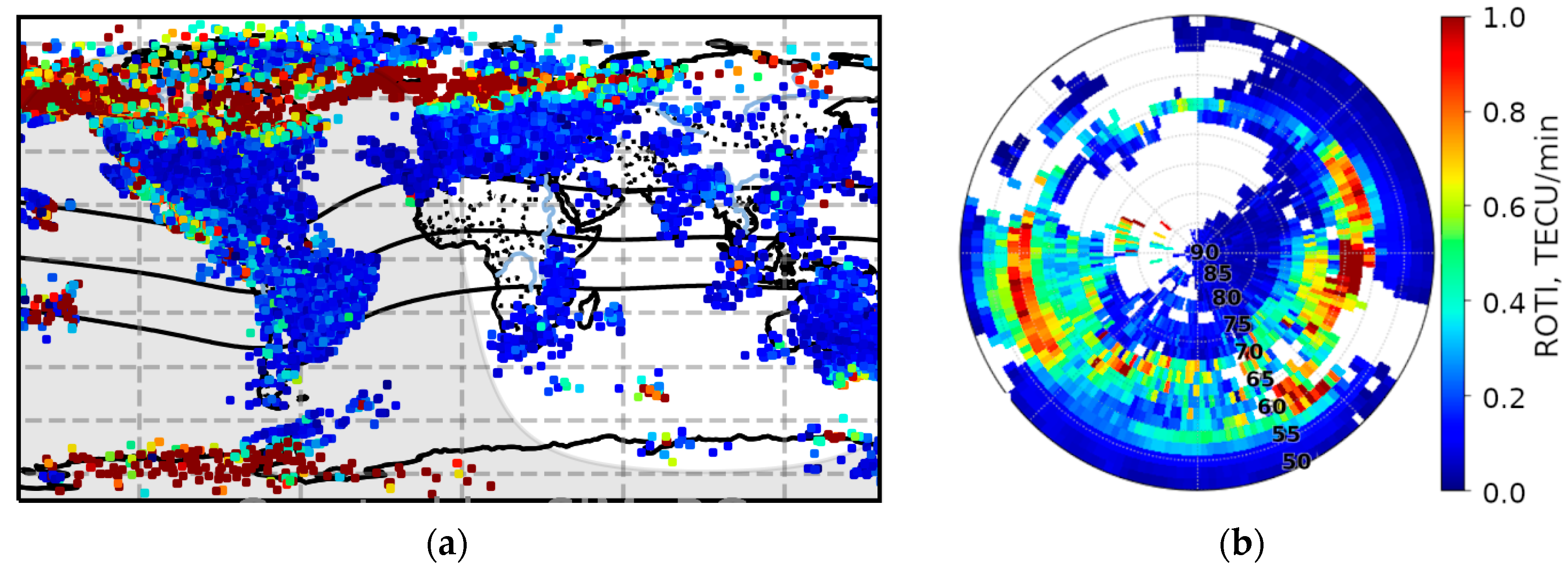
2. Data and Methods
3. Variations in ROTI during Magnetic Storms of 2017–2021 Solar Minimum
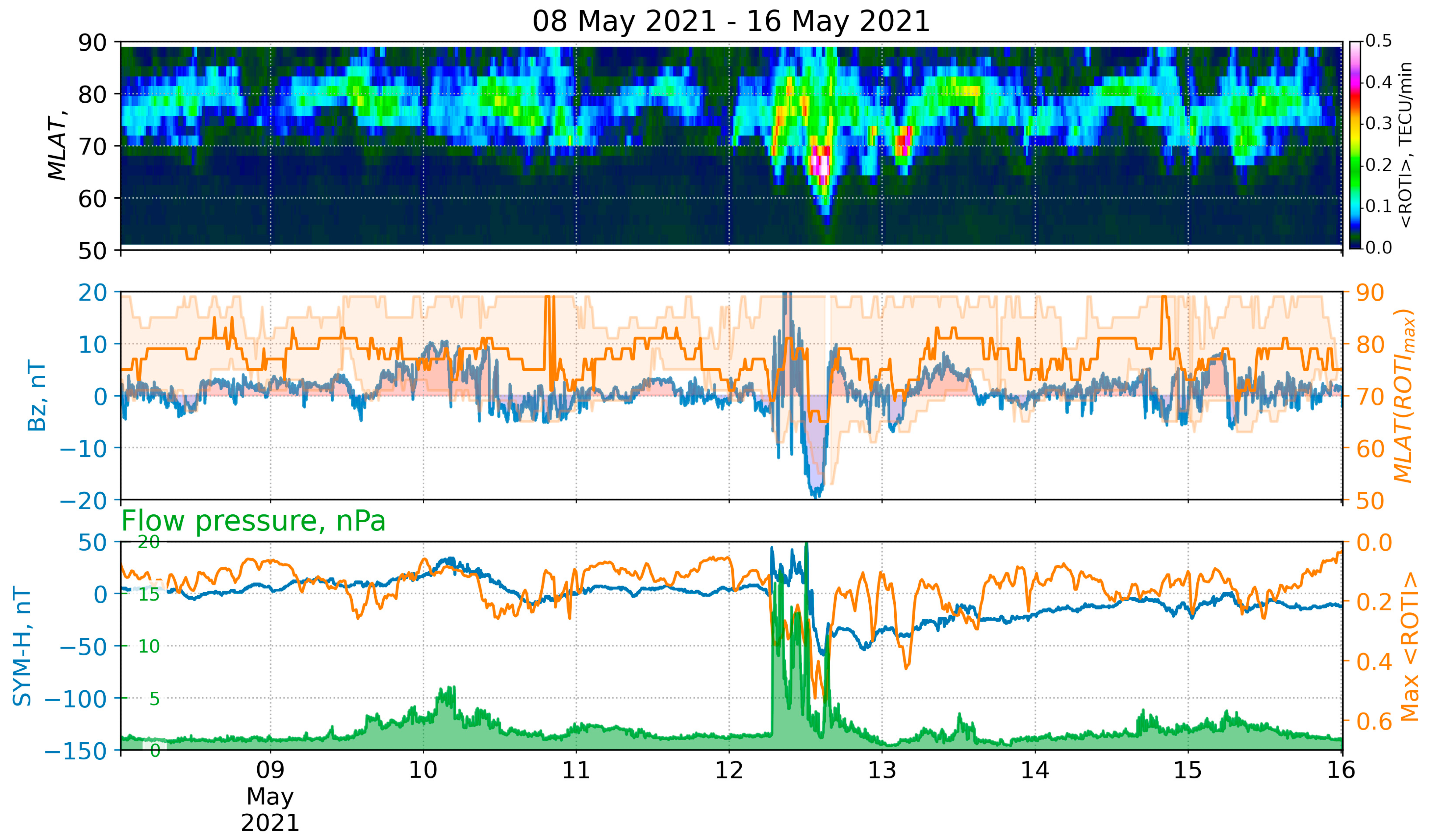
3.1. 12 May 2021 G3 Storm
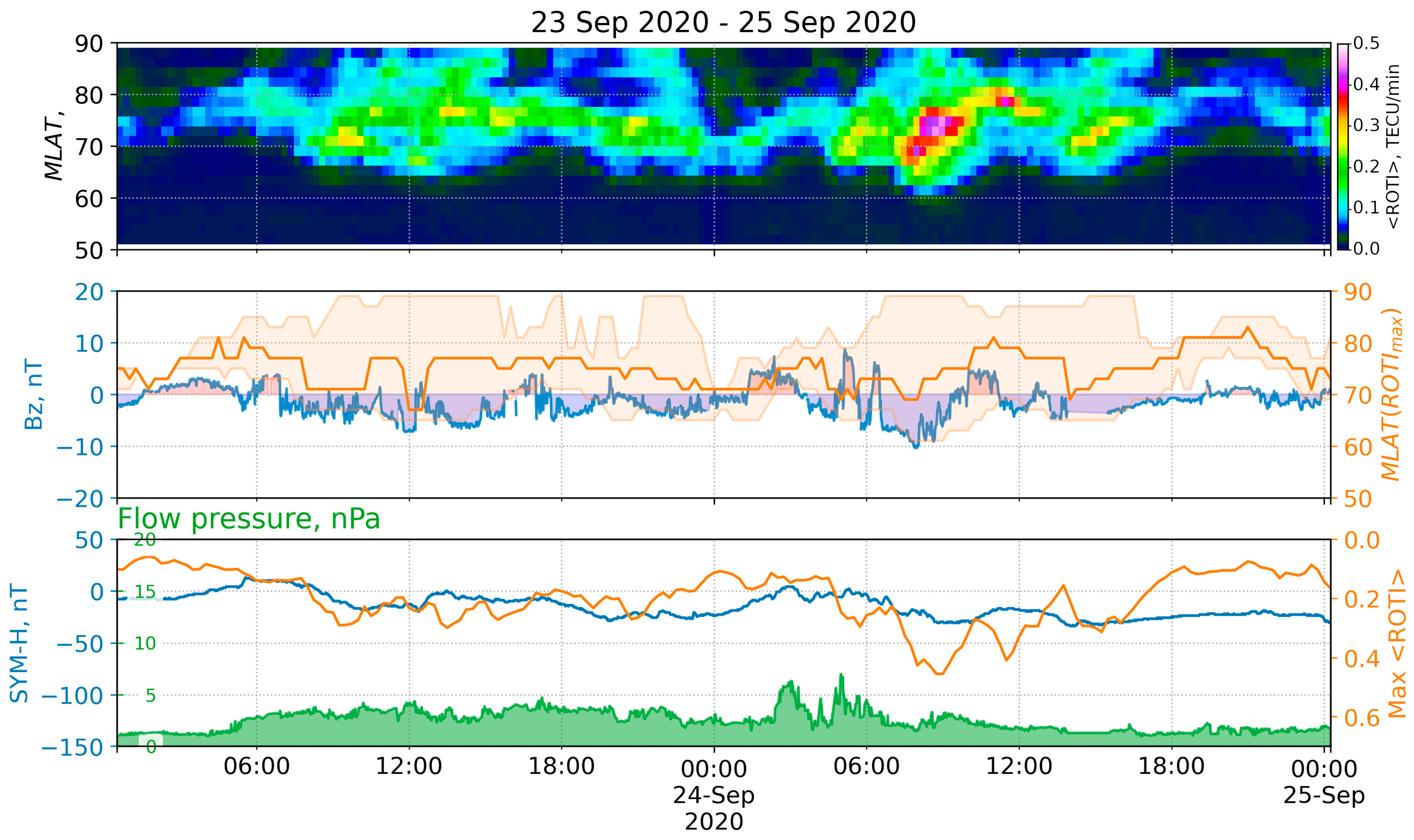
3.2. 24 September 2020 G2 Storm
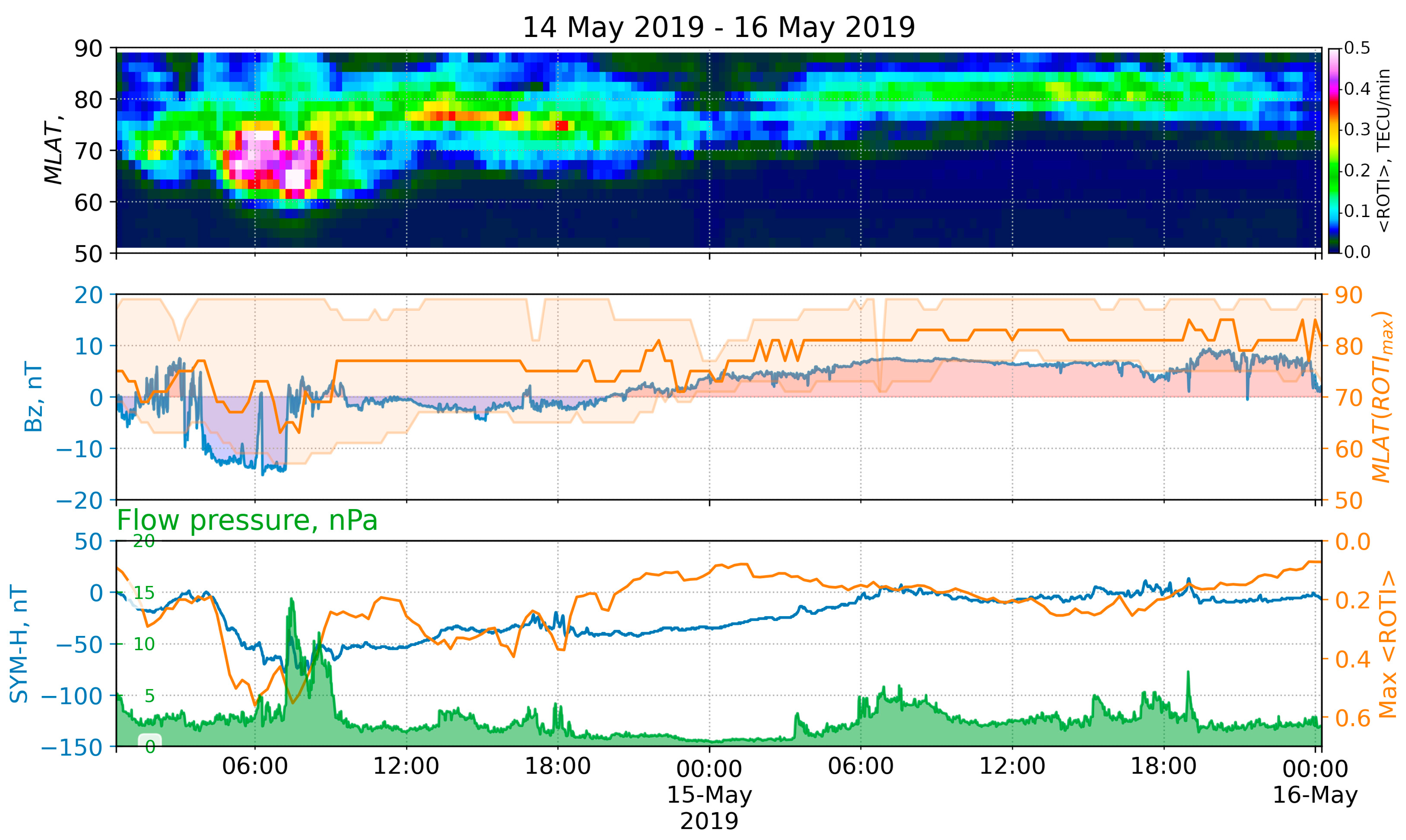
3.3. 14 May 2019 G3 Storm
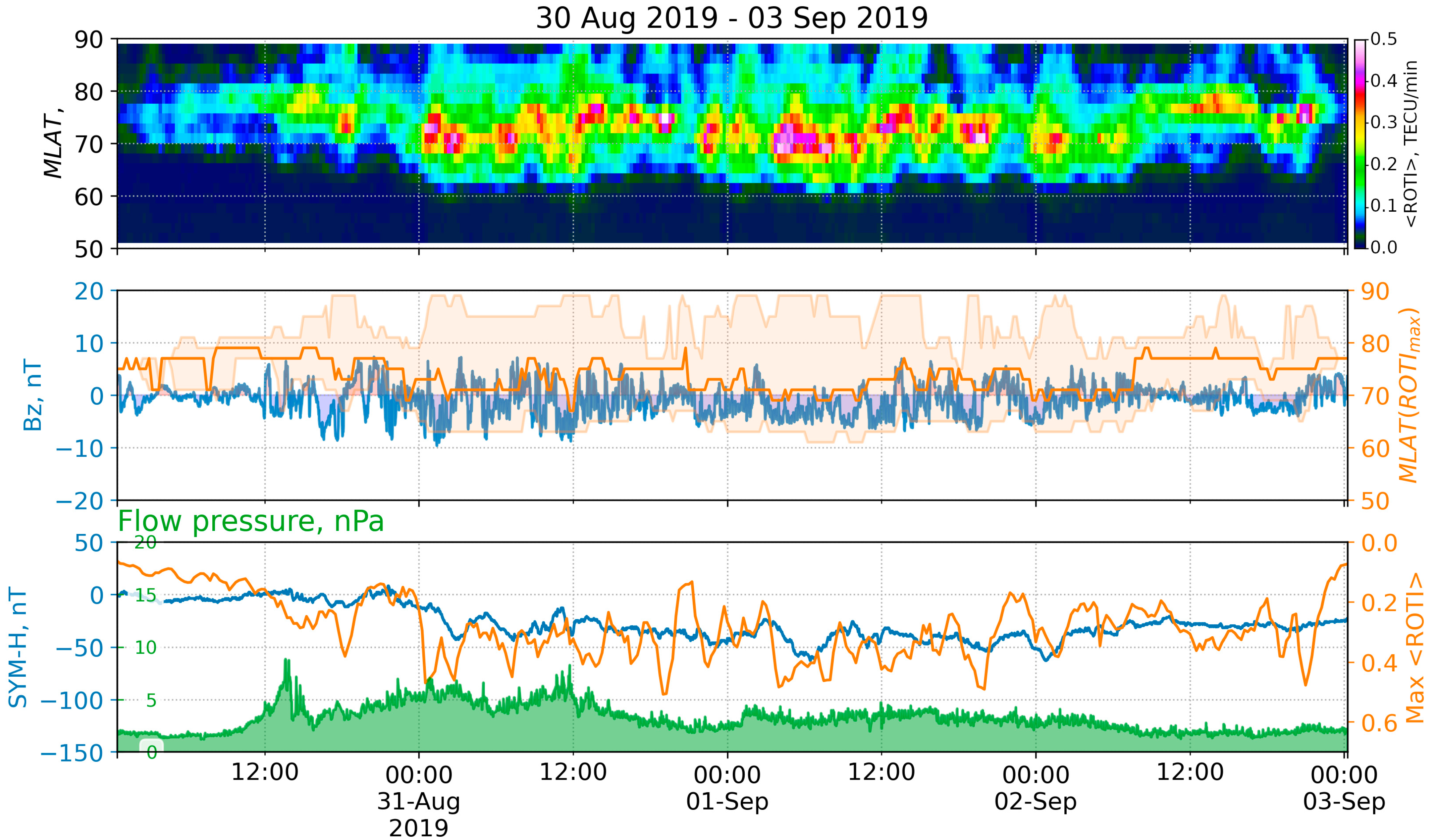
3.4. G2 Storm on 31 August –2 September 2019
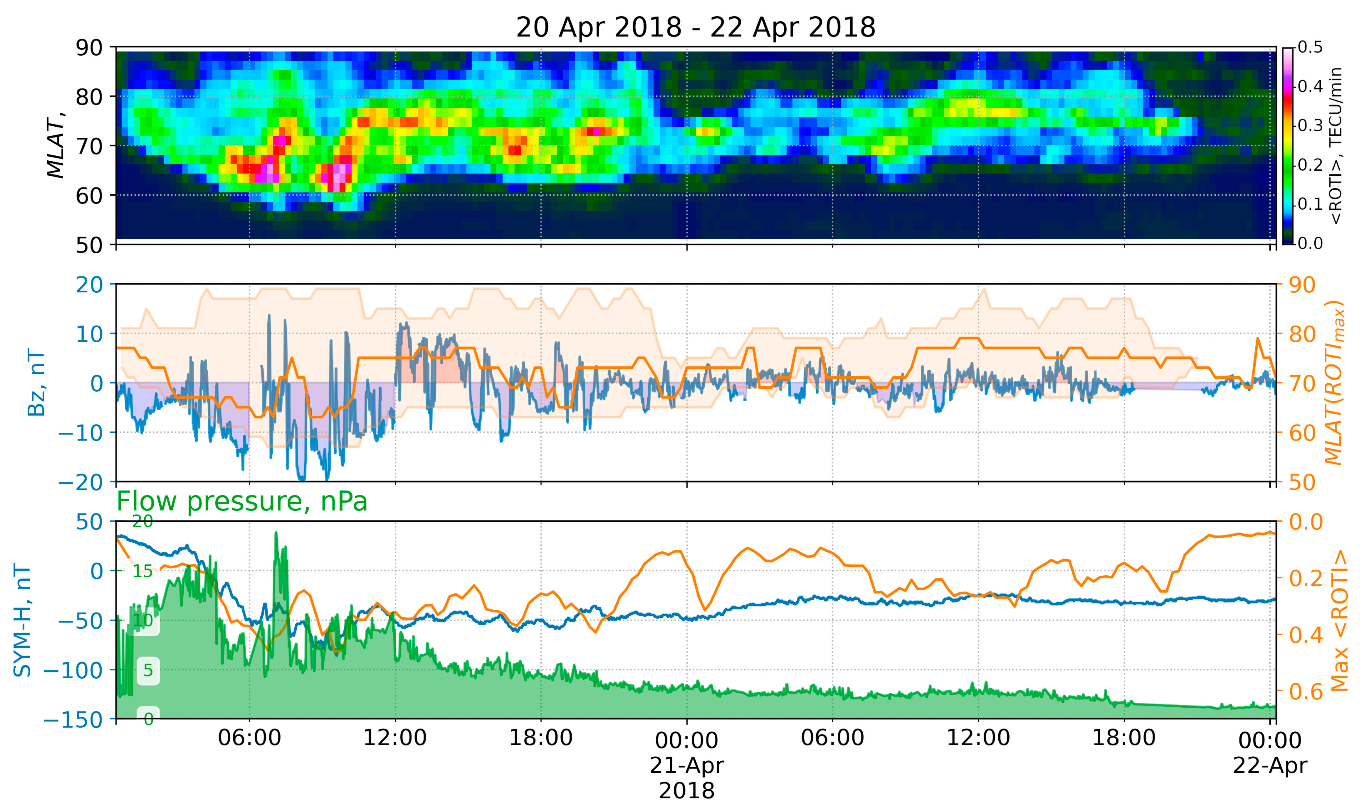
3.5. 20 April 2018 G2 Storm
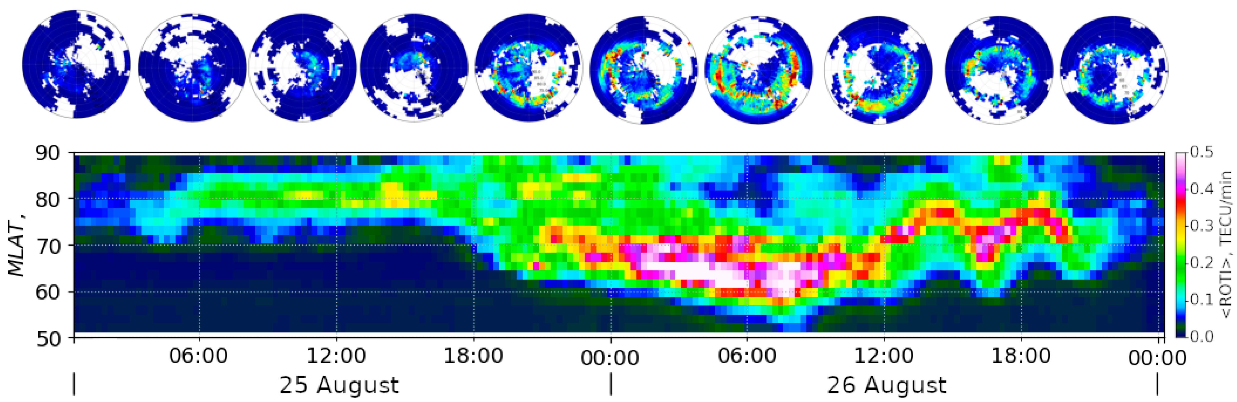
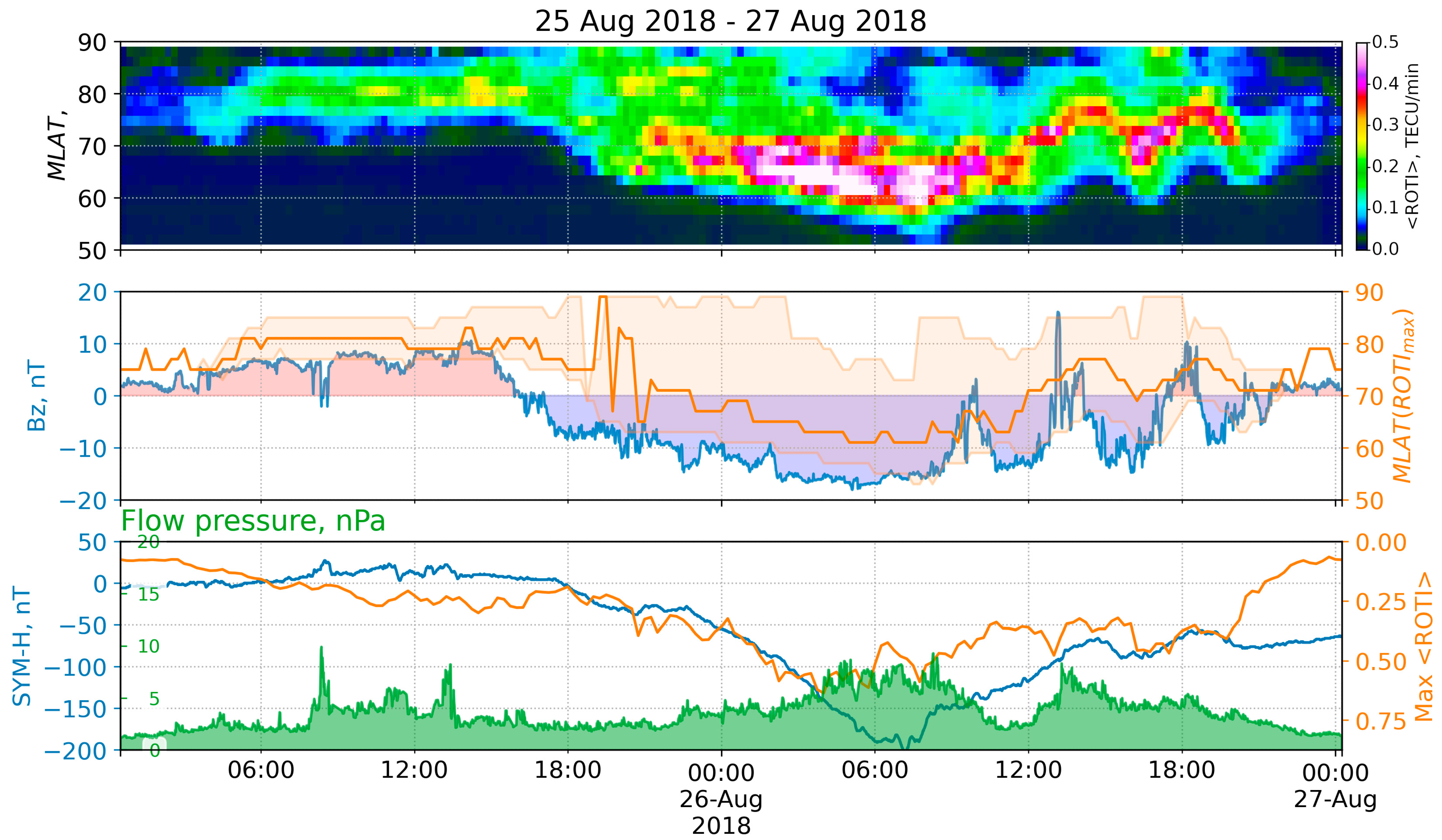
3.6. 25–26 August 2018 G3 Storm
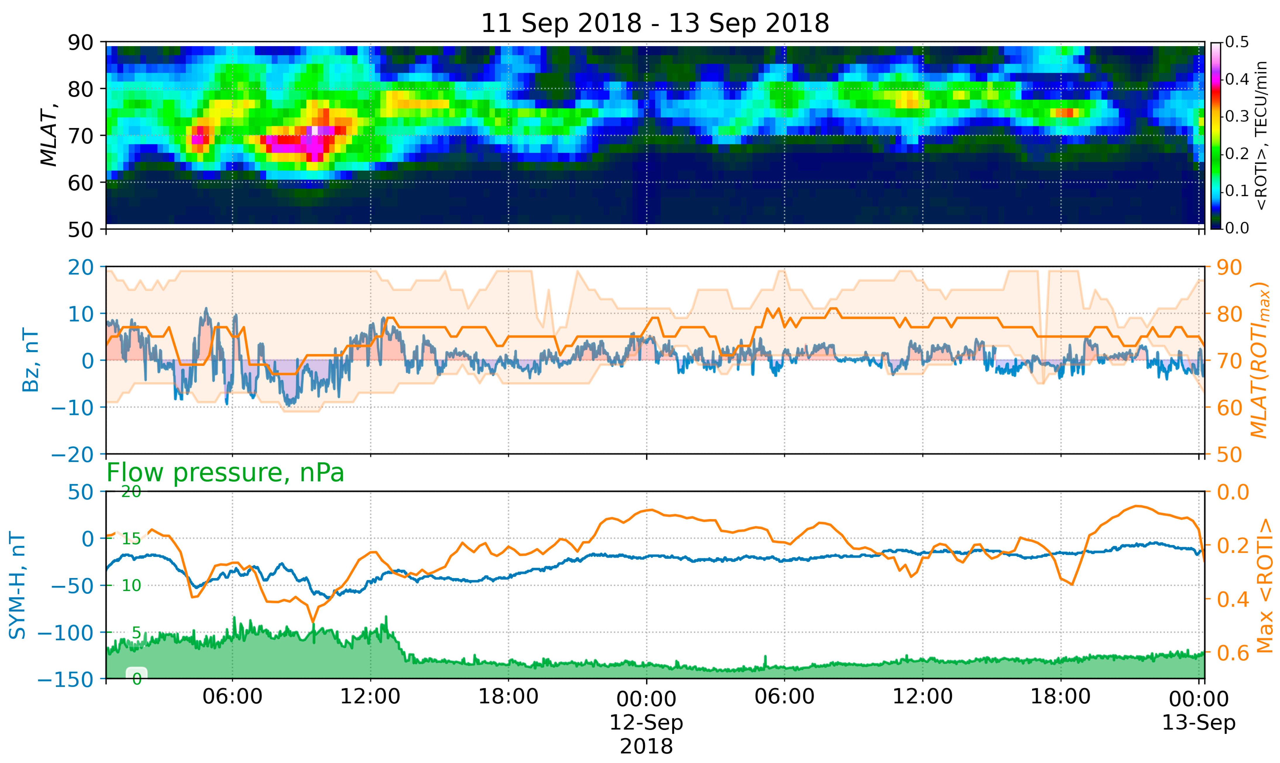
3.7. 11 September 2018 G2 Storm
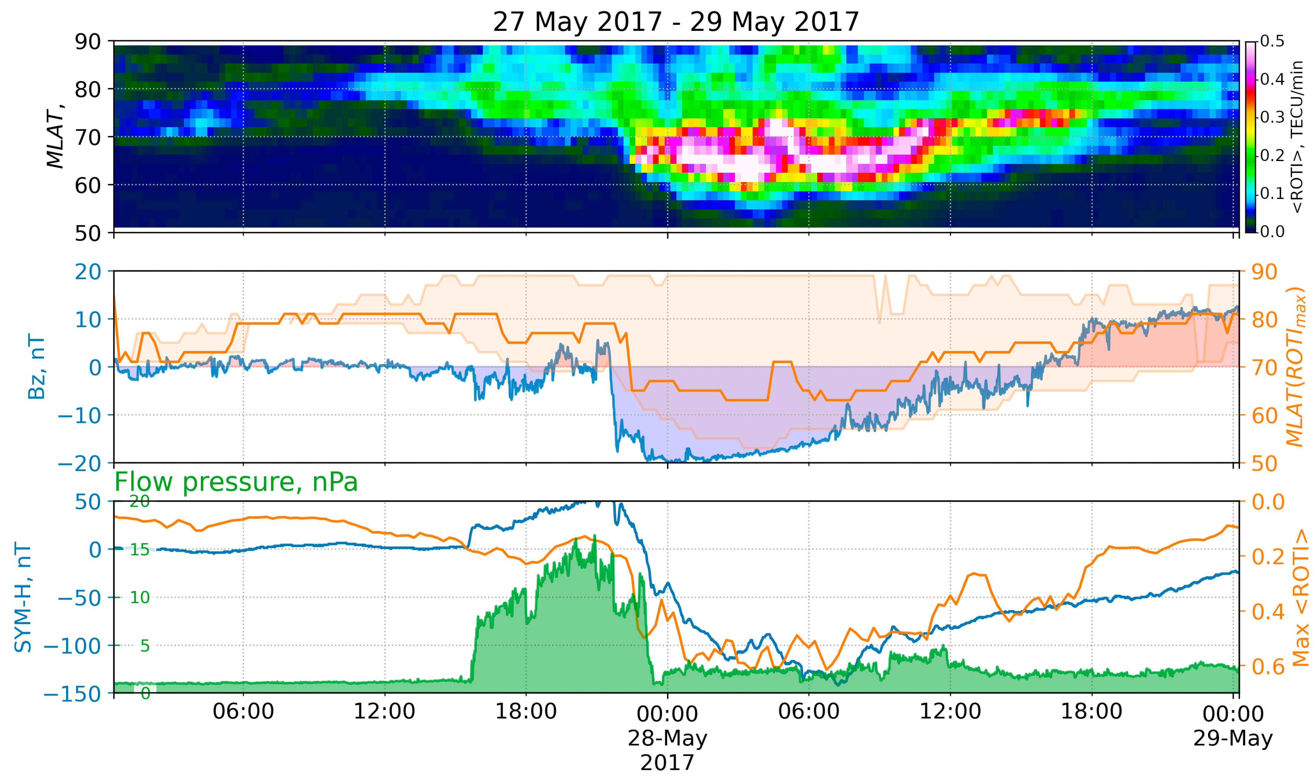
3.8. 27 May 2017 G3 Storm
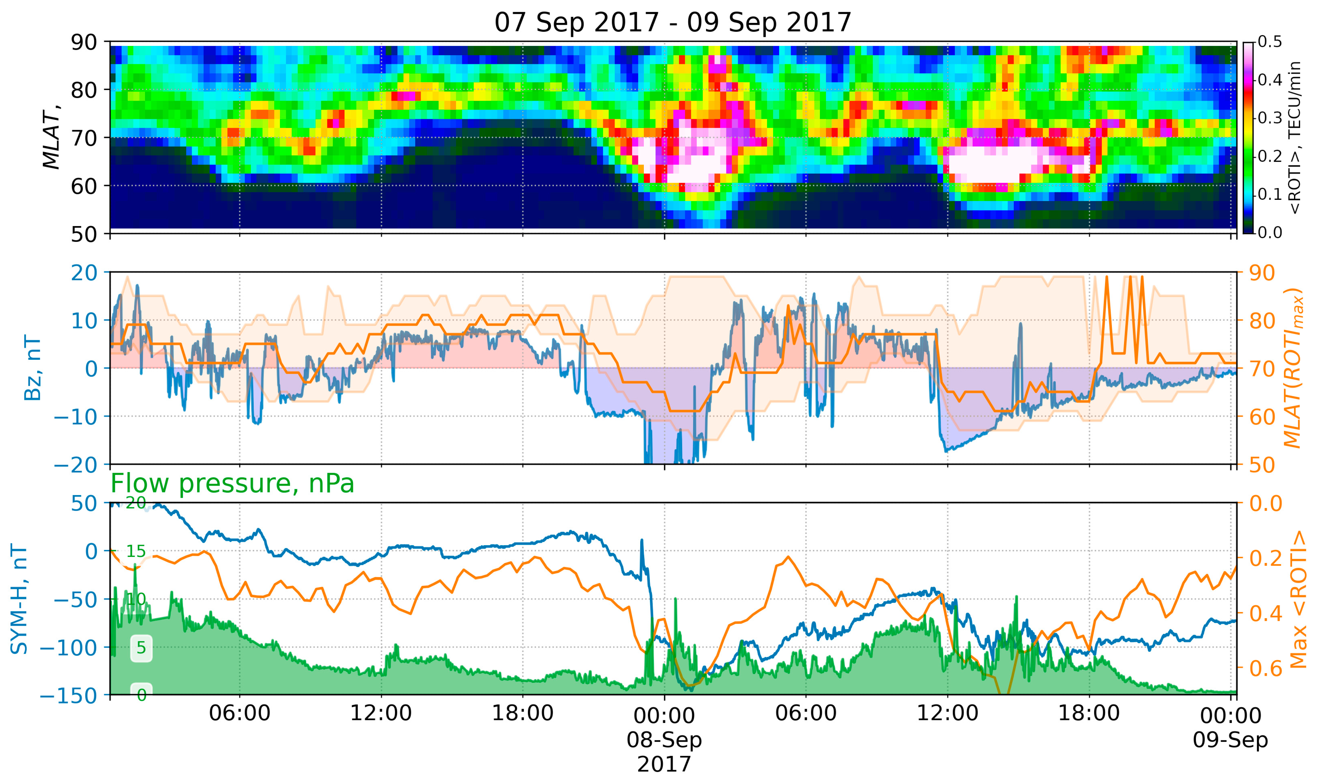
3.9. 7–8 September 2017 G4 Storm
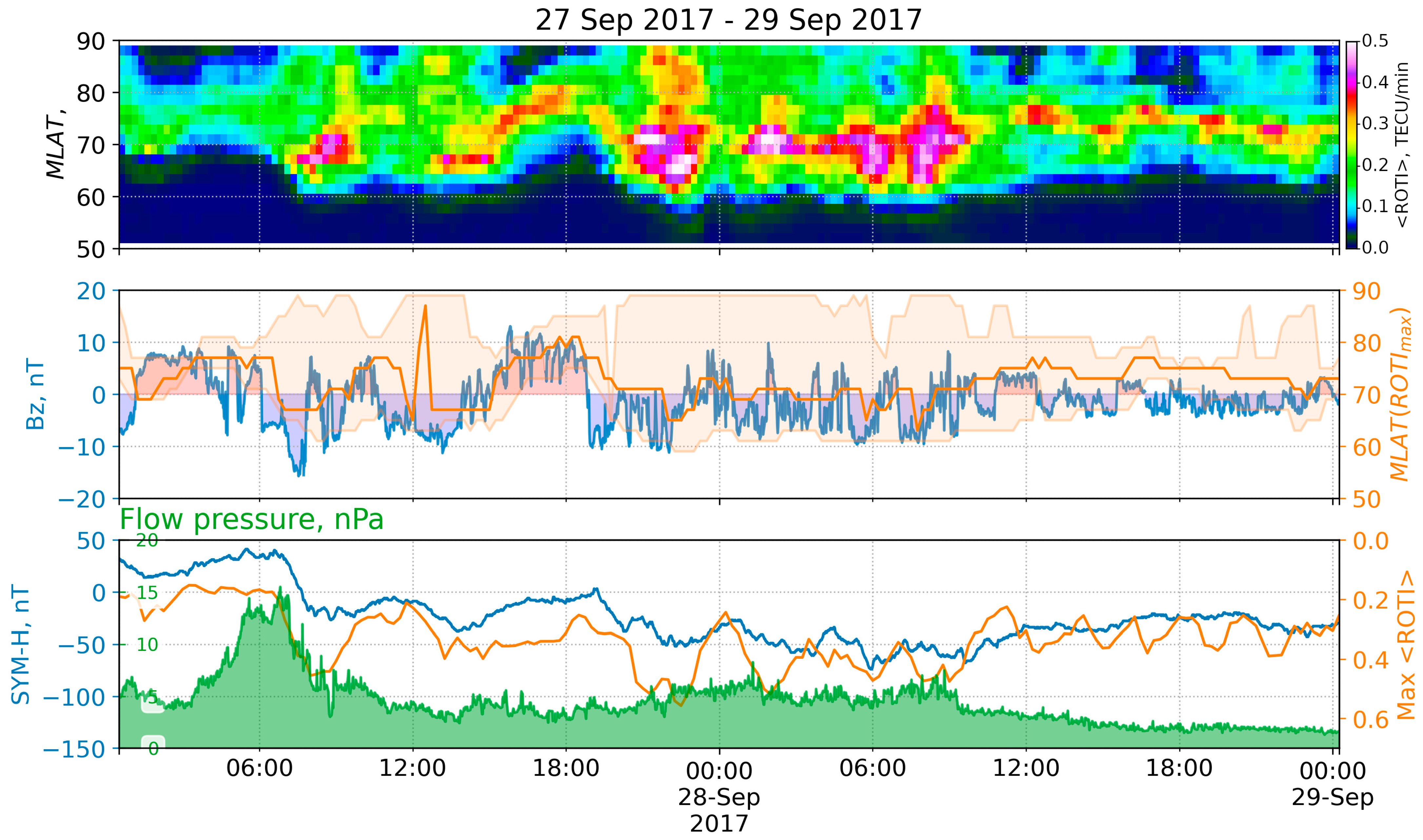
3.10. 27 September 2017 Storm
4. Results
5. Discussion
- CME-driven storms are brief, have denser plasma sheets, have stronger ring currents and Dst perturbation, have solar energetic particle events, and can produce new radiation belts, great auroras, and dangerous geomagnetically induced currents. One might identify CME-driven storms by the stronger magnetic field, enhanced solar wind speed, and low proton temperature [12].
- CIR-driven storms are of longer duration, have hotter plasma sheets and, hence, stronger spacecraft charging, and produce higher fluxes of relativistic electrons. Long-lasting Joule heating during HSS increases the temperature in the ionosphere, changes the recombination coefficient, and speeds up the formation of ionosphere irregularities in the auroral region [49]. This produces long-lasting high ROTI values during HSS, which can be observed in Figure 5, Figure 7, Figure 8, Figure 10, and Figure 13.
6. Conclusions
- (1)
- The main phase of the storm is always accompanied by maximal <ROTI> values.
- (2)
- The magnetic latitude of the highest ROTI decreases with a magnetic storm development.
- (3)
- Mostly, the variations in the Bz agree with the variations in the magnetic latitude of the maximal ROTI values.
- (4)
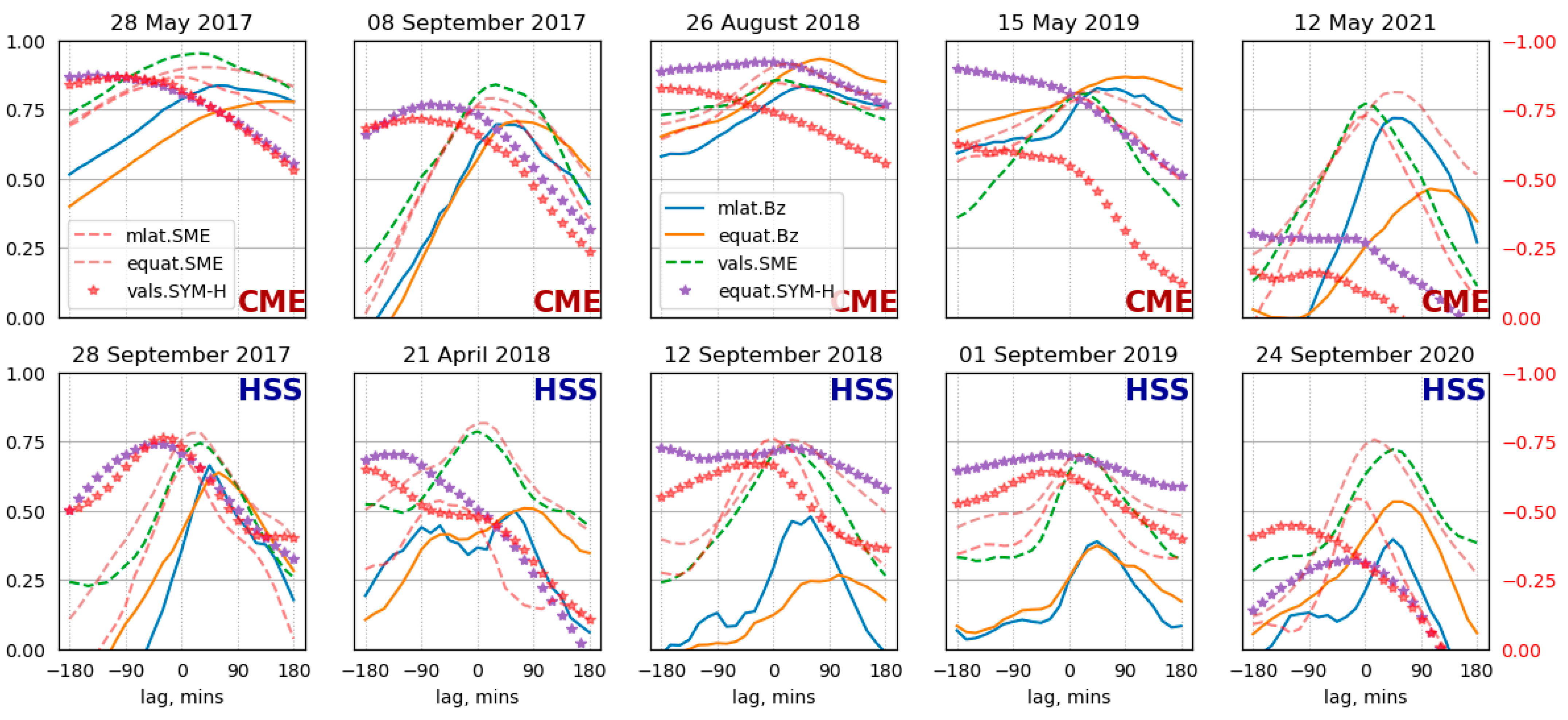
- The highest cross-correlations are observed with a lag of 1 h, between the IMF z-component Bz and the magnetic latitude where the highest ROTI values appear.
- (5)
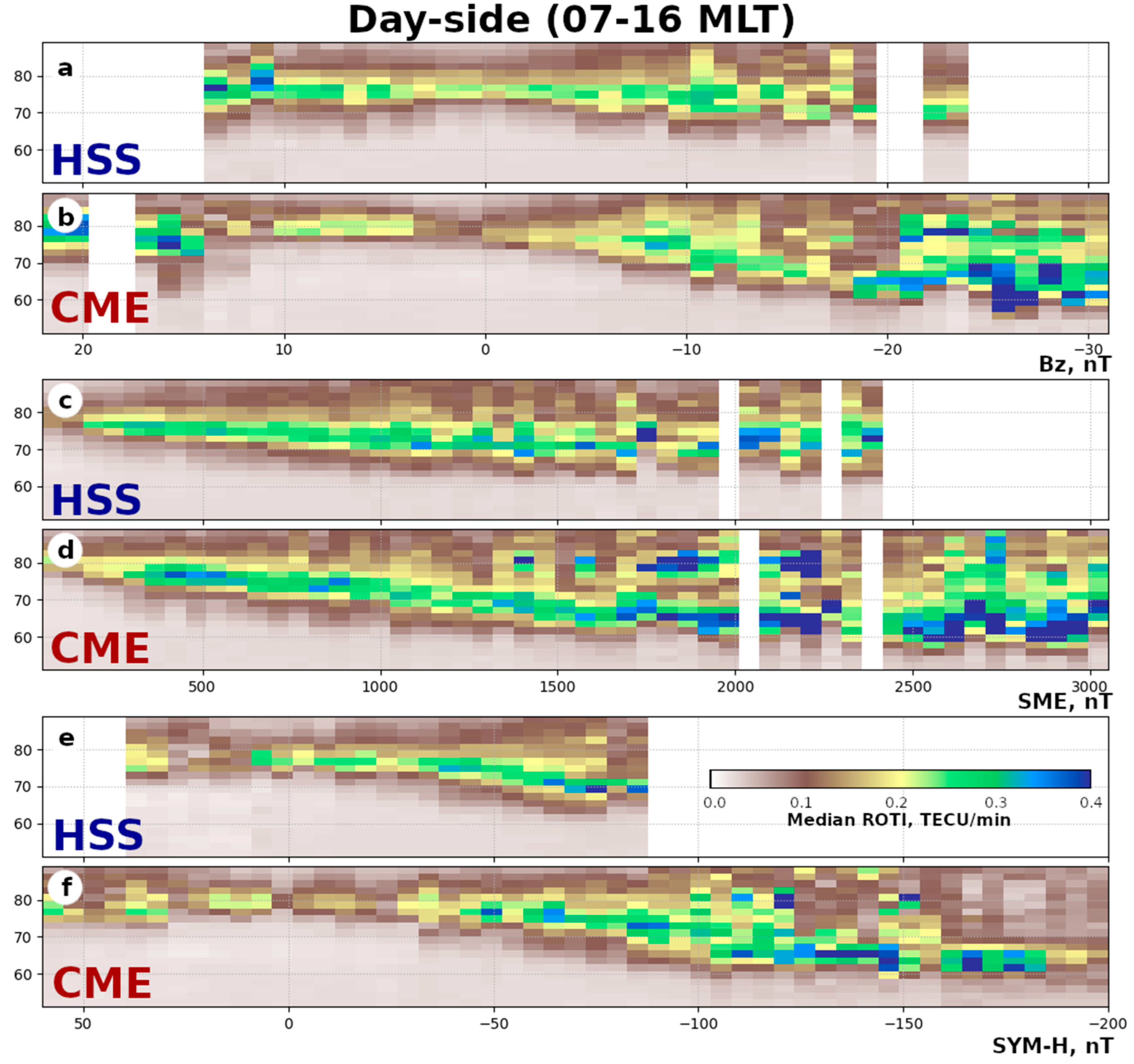
- The auroral electrojet (SME index) shows the highest impact on the ROTI dynamics.
- (6)
- An increase in the space weather indices (in absolute value) is accompanied by a decrease in the latitude where the maximal ROTI occurs (except for proton-density effects).
- (7)
- Even at a small negative Bz, we observe accumulating energy and an increase in the ROTI values.
- (1)
- All the CME-driven storms feature high cross-correlation (>0.75) between the IMF z-component Bz and the magnetic latitude where the highest ROTI appears, while the HSS-driven storms feature a lower cross-correlation (<0.75) between them.
- (2)
- The difference in the duration of similar (by maximal values of geomagnetic indices) HSS- and CME-driven storms could produce differences in the highest ROTI values.
- (3)
- Correlations show that CME-driven storms impact the ROTI values and locations of regions with a high ROTI more directly compared with HSS-driven storms.
- (4)
- CME-driven storms feature higher ROTI values compared with HSS-driven ones at the same level of geomagnetic activity.
Author Contributions
Funding
Data Availability Statement
Acknowledgments
Conflicts of Interest
References
- Chisham, G.; Lester, M.; Milan, S.E.; Freeman, M.P.; Bristow, W.A.; Grocott, A.; McWilliams, K.A.; Ruohoniemi, J.M.; Yeoman, T.K.; Dyson, P.L.; et al. A decade of the Super Dual Auroral Radar Network (SuperDARN): Scientific achievements, new techniques and future directions. Surv. Geophys. 2007, 28, 33–109. [Google Scholar] [CrossRef] [Green Version]
- Imber, S.M.; Milan, S.E.; Lester, M. The Heppner-Maynard Boundary measured by SuperDARN as a proxy for the latitude of the auroral oval. J. Geophys. Res. Space Phys. 2013, 118, 685–697. [Google Scholar] [CrossRef] [Green Version]
- Pi, X.; Mannucci, A.J.; Lindqwister, U.J.; Ho, C.M. Monitoring of global ionospheric irregularities using the Worldwide GPS Network. Geophys. Res. Lett. 1997, 24, 2283–2286. [Google Scholar] [CrossRef]
- Astafyeva, E.; Yasyukevich, Y.V.; Maletckii, B.; Oinats, A.; Vesnin, A.; Yasyukevich, A.S.; Syrovatskii, S.; Guendouz, N. Ionospheric disturbances and irregularities during the 25–26 August 2018 geomagnetic storm. J. Geophys. Res. Space Phys. 2022, 127, e2021JA029843. [Google Scholar] [CrossRef]
- Tsugawa, T.; Nishioka, M.; Ishii, M.; Hozumi, K.; Saito, S.; Shinbori, A.; Otsuka, Y.; Saito, A.; Buhari, S.M.; Abdullah, M. Total Electron Content Observations by Dense Regional and Worldwide International Networks of GNSS. J. Disaster Res. 2018, 13, 535–545. [Google Scholar] [CrossRef]
- Yasyukevich, Y.; Kiselev, A.V.; Zhivetiev, I.V.; Edemskiy, I.K.; Syrovatskii, S.V.; Maletckii, B.M.; Vesnin, A.M. SIMuRG: System for Ionosphere Monitoring and Research from GNSS. GPS Solut. 2020, 24, 69. [Google Scholar] [CrossRef]
- Cherniak, I.; Krankowski, A.; Zakharenkova, I. ROTI Maps: A new IGS ionospheric product characterizing the ionospheric irregularities occurrence. GPS Solut. 2018, 22, 69. [Google Scholar] [CrossRef]
- Kotulak, K.; Zakharenkova, I.; Krankowski, A.; Cherniak, I.; Wang, N.; Fron, A. Climatology Characteristics of Ionospheric Irregularities Described with GNSS ROTI. Remote Sens. 2020, 12, 2634. [Google Scholar] [CrossRef]
- Sori, T.; Shinbori, A.; Otsuka, Y.; Tsugawa, T.; Nishioka, M. The occurrence feature of plasma bubbles in the equatorial to midlatitude ionosphere during geomagnetic storms using long-term GNSS-TEC data. J. Geophys. Res. Space Phys. 2021, 126, e2020JA029010. [Google Scholar] [CrossRef]
- Li, W.; Song, S.; Jin, X. Ionospheric scintillation monitoring with ROTI from geodetic receiver: Limitations and performance evaluation. Radio Sci. 2022, 57, 1–15. [Google Scholar] [CrossRef]
- Sieradzki, R.; Paziewski, J. GNSS-based analysis of high latitude ionospheric response on a sequence of geomagnetic storms performed with ROTI and a new relative STEC indicator. J. Space Weather Space Clim. 2019, 9, A5. [Google Scholar] [CrossRef] [Green Version]
- Dugassa, T.; Habarulema, J.B.; Nigussie, M. Equatorial and low-latitude ionospheric TEC response to CIR-driven geomagnetic storms at different longitude sectors. Adv. Space Res. 2020, 66, 1947–1966. [Google Scholar] [CrossRef]
- Maruyama, T.; Ma, G.; Tsugawa, T. Storm-induced plasma stream in the low-latitude to midlatitude ionosphere. J. Geophys. Res. Space Phys. 2013, 118, 5931–5941. [Google Scholar] [CrossRef]
- Beeck, S.S.; Jensen, A.B.O. ROTI maps of Greenland using kriging. J. Geod. Sci. 2021, 11, 83–94. [Google Scholar] [CrossRef]
- King, J.H.; Papitashvili, N.E. Solar wind spatial scales in and comparisons of hourly Wind and ACE plasma and magnetic field data. J. Geophys. Res. Space Phys. 2005, 110, A02209. [Google Scholar] [CrossRef]
- Gjerloev, J.W. The SuperMAG data processing technique. J. Geophys. Res. Space Phys. 2012, 117, A09213. [Google Scholar] [CrossRef]
- Space Weather Highlights by SWPC for Week 2385 (10–16 May 2021). Available online: ftp://ftp.swpc.noaa.gov/pub/warehouse/2021/WeeklyPDF/prf3285.pdf (accessed on 29 September 2022).
- Space Weather Highlights by SWPC for Week 2352 (21–27 September 2020). Available online: Ftp://ftp.swpc.noaa.gov/pub/warehouse/2020/2020_WeeklyPDF.tar.gz/prf2352.pdf (accessed on 29 September 2022).
- Space Weather Highlights by SWPC for Week 2281 (13–19 May 2019). Available online: Ftp://ftp.swpc.noaa.gov/pub/warehouse/2019/2019_WeeklyPDF.tar.gz/prf2281.pdf (accessed on 29 September 2022).
- Chernogor, L.F.; Garmash, K.P.; Guo, Q.; Luo, Y.; Rozumenko, V.T.; Zheng, Y. Ionospheric storm effects over the People’s Republic of China on 14 May 2019: Results from multipath multi-frequency oblique radio sounding. Adv. Space Res. 2020, 66, 226–242. [Google Scholar] [CrossRef]
- Luo, Y.; Chernogor, L.; Garmash, K.; Guo, Q.; Rozumenko, V.; Zheng, Y. Dynamic processes in the magnetic field and in the ionosphere during the 30 August–2 September 2019 geospace storm: Influence on high frequency radio wave characteristics. Ann. Geophys. 2021, 39, 657–685. [Google Scholar] [CrossRef]
- Space Weather Highlights by SWPC for Week (26 August–1 September 2019). Available online: Ftp://ftp.swpc.noaa.gov/pub/warehouse/2019/2019_WeeklyPDF.tar.gz/prf2296.pdf (accessed on 29 September 2022).
- Velinov, P.I.Y.; Tassev, Y.; Tomova, D.; Mateev, L. Analysis and characteristics of unpredictable G2—Moderate geomagnetic storm on 20 April 2018 in solar cycle 24 minimum. C. R. Acad. Bulg. Sci. 2018, 71, 1357–1365. [Google Scholar] [CrossRef]
- Piersanti, M.; De Michelis, P.; Del Moro, D.; Tozzi, R.; Pezzopane, M.; Consolini, G.; Marcucci, M.F.; Laurenza, M.; Di Matteo, S.; Pignalberi, A.; et al. From the Sun to Earth: Effects of the 25 August 2018 geomagnetic storm. Ann. Geophys. 2020, 38, 703–724. [Google Scholar] [CrossRef]
- Blagoveshchensky, D.V.; Sergeeva, M.A. Impact of geomagnetic storm of 7–8 September 2017 on ionosphere and HF propagation: A multi-instrument study. Adv. Space Res. 2019, 63, 239–256. [Google Scholar] [CrossRef]
- Astafyeva, E.; Bagiya, M.S.; Förster, M.; Nishitani, N. Unprecedented Hemispheric Asymmetries During a Surprise Ionospheric Storm: A Game of Drivers. J. Geophys. Res. Space Phys. 2020, 125, e2019JA027261. [Google Scholar] [CrossRef]
- Space Weather Highlights by SWPC for Week 2246 (10–16 September 2018). Available online: Ftp://ftp.swpc.noaa.gov/pub/warehouse/2018/2018_WeeklyPDF.tar.gz/prf2246.pdf (accessed on 29 September 2022).
- Space Weather Highlights by SWPC for Week 2178 (22–28 May 2017). Available online: Ftp://ftp.swpc.noaa.gov/pub/warehouse/2017/2017_WeeklyPDF.tar.gz/prf2178.pdf (accessed on 29 September 2022).
- Ovodenko, V.B.; Klimenko, M.V.; Zakharenkova, I.E.; Oinats, A.V.; Kotova, D.S.; Nikolaev, A.V.; Chernyshov, A.A. Spatial and temporal evolution of different-scale ionospheric irregularities in Central and East Siberia during the 27–28 May 2017 geomagnetic storm. Space Weather 2020, 18, e2019SW002378. [Google Scholar] [CrossRef]
- De Paula, E.R.; de Oliveira, C.M.; Caton, R.G.; Negreti, P.M.; Batista, I.S.; Martinon, A.R.F.; Neto, A.C.; Abdu, M.A.; Monico, J.F.G.; Sousasantos, J.; et al. Ionospheric irregularity behavior during the 6–10 September 2017 magnetic storm over Brazilian equatorial–low latitudes. Earth Planets Space 2019, 71, 42. [Google Scholar] [CrossRef]
- Hajra, R. September 2017 Space-Weather Events: A Study on Magnetic Reconnection and Geoeffectiveness. Sol. Phys. 2021, 296, 50. [Google Scholar] [CrossRef]
- Shinbori, A.; Otsuka, Y.; Sori, T.; Tsugawa, T.; Nishioka, M. Temporal and spatial variations of total electron content enhancements during a geomagnetic storm on 27 and 28 September 2017. J. Geophys. Res. Space Phys. 2020, 125, e2019JA026873. [Google Scholar] [CrossRef]
- Hargreaves, J.K. Auroral radio absorption: The prediction question. Adv. Space Res. 2010, 45, 1075–1092. [Google Scholar] [CrossRef]
- Ruck, J.J.; Themens, D.R. Impacts of auroral precipitation on HF propagation: A hypothetical over-the-horizon radar case study. Space Weather 2021, 19, e2021SW002901. [Google Scholar] [CrossRef]
- Smith, A.M.; Mitchell, C.N.; Watson, R.J.; Meggs, R.W.; Kintner, P.M.; Kauristie, K.; Honary, F. GPS scintillation in the high Arctic associated with an auroral arc. Space Weather 2008, 6, 1–7. [Google Scholar] [CrossRef]
- van der Meeren, C.; Oksavik, K.; Lorentzen, D.A.; Rietveld, M.T.; Clausen, L.B.N. Severe and localized GNSS scintillation at the poleward edge of the nightsideauroral oval during intense substorm aurora. J. Geophys. Res. Space Phys. 2015, 120, 10607–10621. [Google Scholar] [CrossRef]
- Prikryl, P.; Ghoddousi-Fard, R.; Thomas, E.G.; Ruohoniemi, J.M.; Shepherd, S.G.; Jayachandran, P.T.; Danskin, D.W.; Spanswick, E.; Zhang, Y.; Jiao, Y. GPS phase scintillation at high latitudes during geomagnetic storms of 7–17 March 2012—Part 1: The North American sector. Ann. Geophys. 2015, 33, 637–656. [Google Scholar] [CrossRef] [Green Version]
- Demyanov, V.V.; Yasyukevich, Y.V. Space weather: Risk factors for global navigation satellite systems. Sol. -Terr. Phys. 2021, 7, 28–47. [Google Scholar] [CrossRef]
- Hardy, D.A.; Gussenhoven, M.S.; Holeman, E. A statistical model of auroral electron precipitation. J. Geophys. Res. Space Phys. 1985, 90, 4229–4248. [Google Scholar] [CrossRef]
- Newell, P.T.; Liou, K.; Zhang, Y.; Sotirelis, T.; Paxton, L.J.; Mitchell, E.J. OVATION Prime-2013: Extension of auroral precipitation model to higher disturbance levels. Space Weather 2014, 12, 368–379. [Google Scholar] [CrossRef]
- Vorobev, A.V.; Pilipenko, V.A.; Krasnoperov, R.I.; Vorobeva, G.R.; Lorentzen, D.A. Short-term forecast of the auroral oval position on the basis of the “virtual globe” technology. Russ. J. Earth Sci. 2020, 20, ES6001. [Google Scholar] [CrossRef]
- Newell, P.T.; Sotirelis, T.; Wing, S. Seasonal variations in diffuse, monoenergetic, and broadband aurora. J. Geophys. Res. Space Phys. 2010, 115, A03216. [Google Scholar] [CrossRef]
- Lunyushkin, S.B.; Penskikh, Y.V. Diagnostics of the auroral oval boundaries on the basis of the magnetogram inversion technique. Sol. -Terr. Phys. 2019, 5, 88–100. [Google Scholar] [CrossRef]
- Perevalova, N.P.; Romanova, E.B.; Tashchilin, A.V. Detection of high-latitude ionospheric structures using GNSS. J. Atmos. Sol. -Terr. Phys. 2020, 207, 105335. [Google Scholar] [CrossRef]
- Yasyukevich, Y.; Vasilyev, R.; Ratovsky, K.; Setov, A.; Globa, M.; Syrovatskii, S.; Yasyukevich, A.; Kiselev, A.; Vesnin, A. Small-Scale Ionospheric Irregularities of Auroral Origin at Mid-latitudes during the 22 June 2015 Magnetic Storm and Their Effect on GPS Positioning. Remote Sens. 2020, 12, 1579. [Google Scholar] [CrossRef]
- Han, Y.; Han, B.; Hu, Z.; Gao, X.; Zhang, L.; Yang, H.; Li, B. Prediction and variation of the auroral oval boundary based on a deep learning model and space physical parameters. Nonlin. Process. Geophys. 2020, 27, 11–22. [Google Scholar] [CrossRef]
- Vasiliev, A.; Yasyukevich, Y.; Garashchenko, A.; Edemskiy, I.; Vesnin, A.; Sidorov, D. Computer Vision for GNSS-based Detection of the Auroral Oval Boundary. Int. J. Artif. Intell. 2021, 19, 132–151. [Google Scholar]
- Borovsky, J.E.; Denton, M.H. Differences between CME-driven storms and CIR-driven storms. J. Geophys. Res. Space Phys. 2006, 111, A07S08. [Google Scholar] [CrossRef] [Green Version]
- Liu, Y.; Li, Z.; Fu, L.; Wang, J.; Radicella, S.M.; Zhang, C. Analyzing Ionosphere TEC and ROTI Responses on 2010 August High Speed Solar Winds. IEEE Access 2019, 7, 29788–29804. [Google Scholar] [CrossRef]
- Gustafsson, G.; Feldstein, Y.I.; Shevnina, N.F. The auroral orientation curves for the IQSY. Planet. Space Sci. 1969, 17, 1657–1666. [Google Scholar] [CrossRef]
- Milan, S.E.; Hutchinson, J.; Boakes, P.D.; Hubert, B. Influences on the radius of the auroral oval. Ann. Geophys. 2009, 27, 2913–2924. [Google Scholar] [CrossRef] [Green Version]
- Starkov, G.V.; Feldshtein, Y.I. Orientation of extended auroral forms. Geomagn. Aeron. 1967, 7, 72–77. [Google Scholar]
- Jin, S.; Jin, R.; Kutoglu, H. Positive and negative ionospheric responses to the March 2015 geomagnetic storm from BDS observations. J. Geod. 2017, 91, 613–626. [Google Scholar] [CrossRef]
- Shen, C.-S.; Zi, M.-Y.; Wang, J.-S.; Xu, J.-Y.; Liu, S.-L. On the Asymmetry of the Storm-Time Current System in the Ionosphere Between Southern and Northern Hemispheres. Chin. J. Geophys. 2006, 49, 1425–1435. [Google Scholar] [CrossRef]
- Dow, J.M.; Neilan, R.E.; Rizos, C. The International GNSS Service in a changing landscape of Global Navigation Satellite Systems. J. Geod. 2009, 83, 191–198. [Google Scholar] [CrossRef]
- Yasyukevich, Y.V.; Vesnin, A.M.; Perevalova, N.P. SibNet–Siberian Global Navigation Satellite System Network: Current state. Sol. -Terr. Phys. 2018, 4, 63–72. [Google Scholar] [CrossRef]
- Jayachandran, P.T.; Langley, R.; Macdougall, J.; Mushini, S.; Hamza, A.; Mann, I.; Milling, D.; Kale, Z.; Chadwick, R.; Kelly, T.; et al. Canadian High Arctic Ionospheric Network (CHAIN). Radio Sci. 2009, 44, RS0A03. [Google Scholar] [CrossRef]
- Bruyninx, C.; Habrich, H.; Kenyeres, A.W.; Söhne, W.; Stangl, G.; Völksen, C. Enhancement of the EUREF Permanent Network Services and Products. Geod. Planet Earth IAG Symp. 2012, 136, 27–35. [Google Scholar] [CrossRef]


| Date | UT, h | Peak Values | Origin | |||
|---|---|---|---|---|---|---|
| SYM-H * | IMF Bz * | Kp | SME * | |||
| 12 May 2021 | 14:49 | −55 | −18.3 | 70 | - | CME |
| 24 September 2020 | 8:50 | −31 | −10 | 6− | 1411 | CH HSS |
| 14 May 2019 | 7:54 | −80 | −15.25 | 6+ | 2015 | CME |
| 1 September 2019 | 6:27 | −62 | −9.7 | 6− | 2309 | CH HSS |
| 20 April 2018 | 9:35 | −86 | −20.9 | 60 | 1892 | −CH HSS |
| 26 August 2018 | 7:10 | −205 | −18 | 7+ | 2587 | CME |
| 11 September 2018 | 10:07 | −64 | −12.6 | 60 | 1974 | +CH HSS |
| 28 May 2017 | 7:13 | −141 | −19.5 | 70 | 2104 | CME |
| 8 September 2017 | 1:08 | −146 | −30 | 8+ | 4455 | CME |
| 28 September 2017 | 5:55 | −74 | −15.7 | 7− | 2126 | CIR HSS |
| Maximal ROTI Values Versus | Latitude of Maximal ROTI Versus | Latitude of Equatorward Boundary Versus | ||||||
|---|---|---|---|---|---|---|---|---|
| Date | SYM-H | SME | Bz | SME | Bz | SYM-H | SME | |
| CME | 12 May 2021 | −0.17 | 0.77 | 0.72 | −0.73 | 0.46 | 0.30 | −0.81 |
| 14 May 2019 | −0.63 | 0.81 | 0.83 | −0.79 | 0.87 | 0.90 | −0.82 | |
| 26 August 2018 | −0.83 | 0.86 | 0.83 | −0.85 | 0.93 | 0.92 | −0.91 | |
| 28 May 2017 | −0.87 | 0.95 | 0.84 | −0.87 | 0.78 | 0.87 | −0.90 | |
| 8 September 2017 | −0.72 | 0.84 | 0.70 | −0.76 | 0.71 | 0.77 | −0.79 | |
| HSS | 24 September 2020 | −0.45 | 0.72 | 0.40 | −0.54 | 0.53 | 0.32 | −0.76 |
| 1 Septemer 2019 | −0.64 | 0.70 | 0.39 | −0.60 | 0.37 | 0.70 | −0.70 | |
| 11 September 2018 | −0.67 | 0.74 | 0.48 | −0.76 | 0.27 | 0.73 | −0.76 | |
| 20 April 2018 | −0.65 | 0.79 | 0.50 | −0.54 | 0.51 | 0.71 | −0.82 | |
| 28 September 2017 | −0.77 | 0.74 | 0.66 | −0.66 | 0.64 | 0.74 | −0.78 | |
Publisher’s Note: MDPI stays neutral with regard to jurisdictional claims in published maps and institutional affiliations. |
© 2022 by the authors. Licensee MDPI, Basel, Switzerland. This article is an open access article distributed under the terms and conditions of the Creative Commons Attribution (CC BY) license (https://creativecommons.org/licenses/by/4.0/).
Share and Cite
Edemskiy, I.K.; Yasyukevich, Y.V. Auroral Oval Boundary Dynamics on the Nature of Geomagnetic Storm. Remote Sens. 2022, 14, 5486. https://doi.org/10.3390/rs14215486
Edemskiy IK, Yasyukevich YV. Auroral Oval Boundary Dynamics on the Nature of Geomagnetic Storm. Remote Sensing. 2022; 14(21):5486. https://doi.org/10.3390/rs14215486
Chicago/Turabian StyleEdemskiy, Ilya K., and Yury V. Yasyukevich. 2022. "Auroral Oval Boundary Dynamics on the Nature of Geomagnetic Storm" Remote Sensing 14, no. 21: 5486. https://doi.org/10.3390/rs14215486