
Decadal Continuous Meteor-Radar Estimation of the Mesopause Gravity Wave Momentum Fluxes over Mohe: Capability Evaluation and Interannual Variation
 , , ,
, , ,
Abstract
:1. Introduction
2. Materials and Methods
3. Results
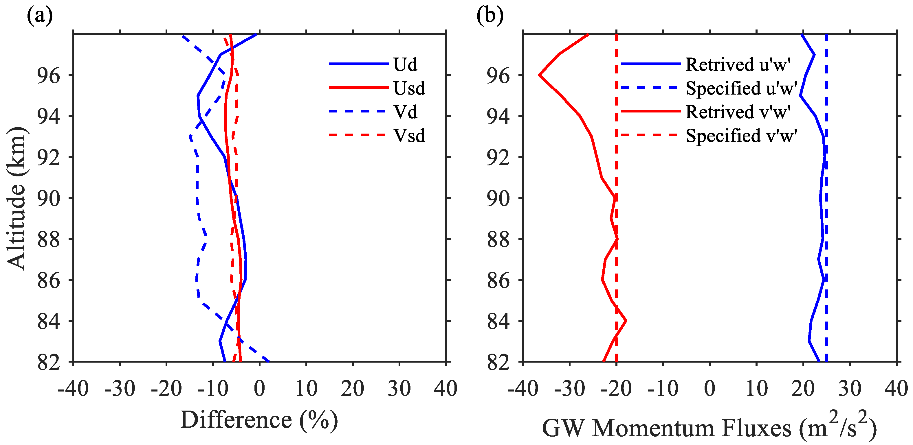
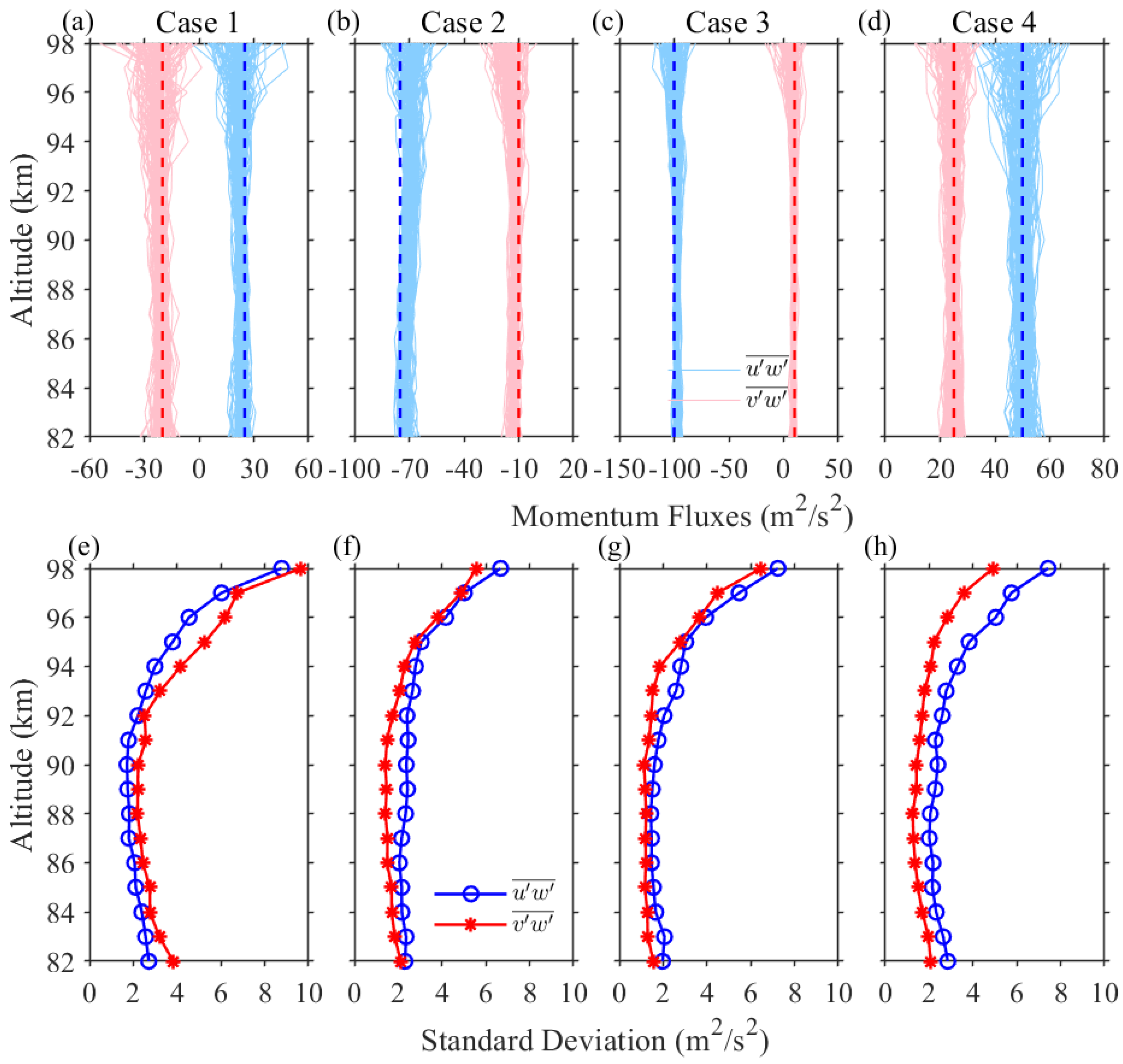
3.1. Case 1
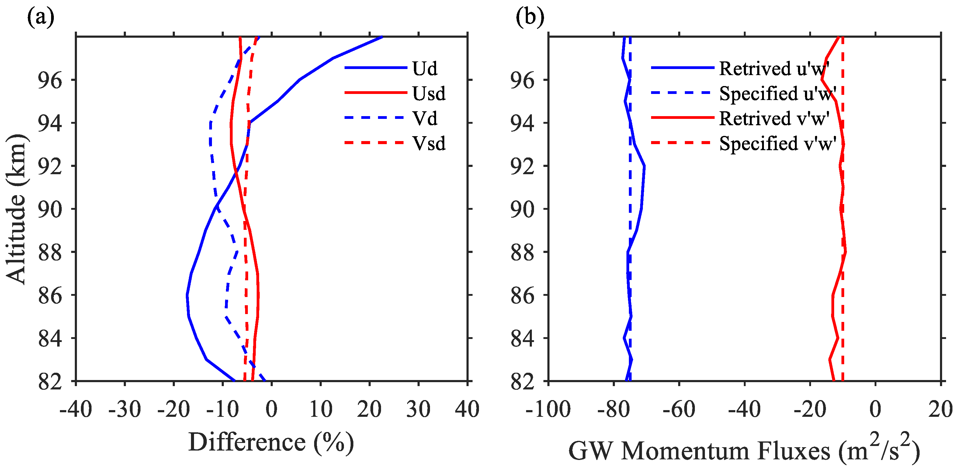
3.2. Case 2
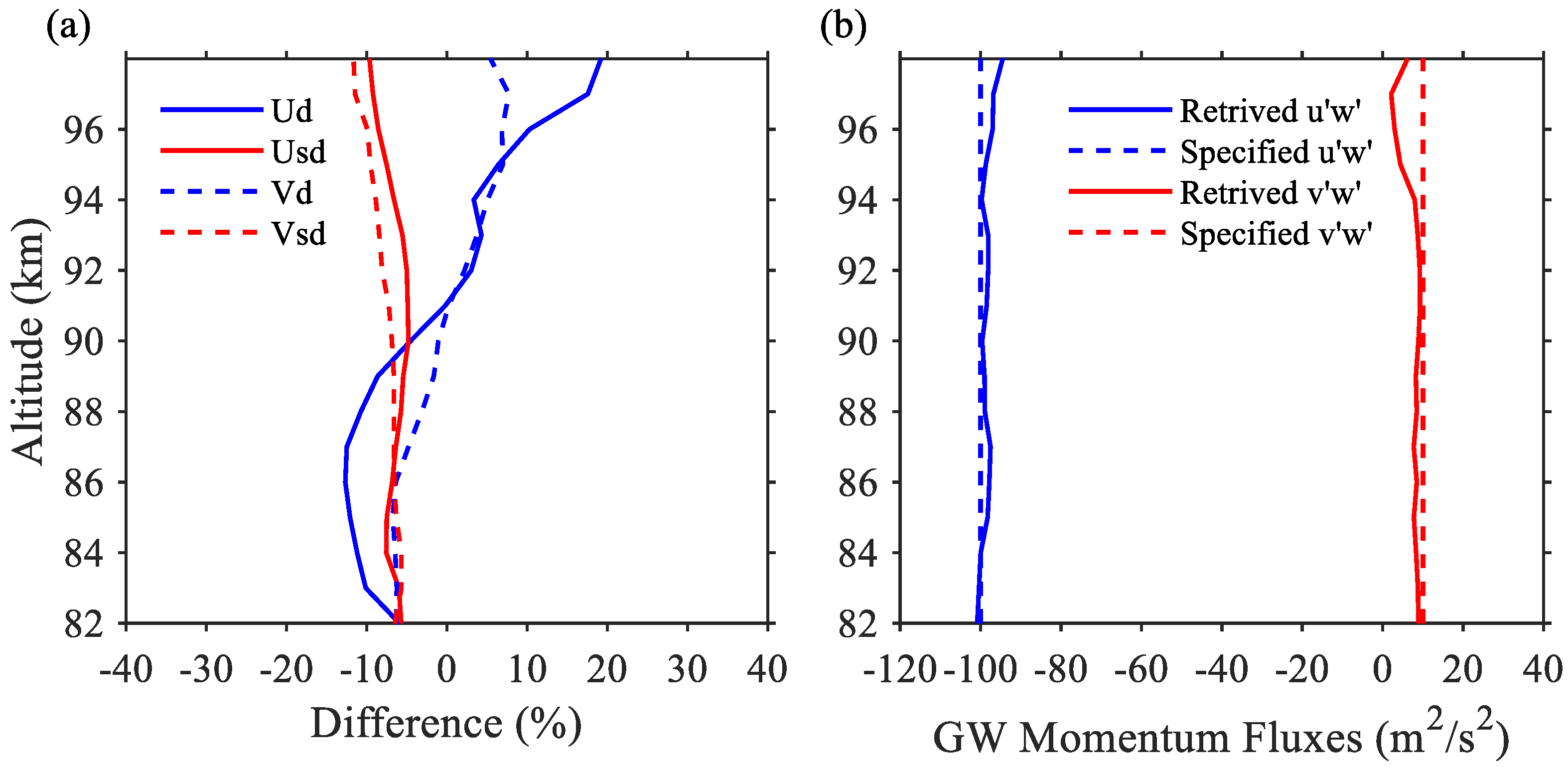
3.3. Case 3
3.4. Case 4
4. Discussion
5. Conclusions
Author Contributions
Funding
Data Availability Statement
Acknowledgments
Conflicts of Interest
References
- Fritts, D.C.; Alexander, M.J. Gravity wave dynamics and effects in the middle atmosphere. Rev. Geophys. 2003, 41, 1003. [Google Scholar] [CrossRef] [Green Version]
- Liu, A.Z.; Lu, X.; Franke, S.J. Diurnal variation of gravity wave momentum flux and its forcing on the diurnal tide. J. Geophys. Res. Atmos. 2013, 118, 1668–1678. [Google Scholar] [CrossRef] [Green Version]
- De Wit, R.; Hibbins, R.; Espy, P. The seasonal cycle of gravity wave momentum flux and forcing in the high latitude northern hemisphere mesopause region. J. Atmos. Sol.-Terr. Phys. 2015, 127, 21–29. [Google Scholar] [CrossRef]
- Placke, M.; Stober, G.; Jacobi, C. Gravity wave momentum fluxes in the MLT—Part I: Seasonal variation at Collm (51.3°N, 13.0°E). J. Atmos. Sol.-Terr. Phys. 2011, 73, 904–910. [Google Scholar] [CrossRef]
- Tsuchiya, C.; Sato, K.; Alexander, M.J.; Hoffmann, L. MJO-related intraseasonal variation of gravity waves in the Southern Hemisphere tropical stratosphere revealed by high-resolution AIRS observations. J. Geophys. Res. Atmos. 2016, 121, 7641–7651. [Google Scholar] [CrossRef] [Green Version]
- De Wit, R.J.; Janches, D.; Fritts, D.C.; Hibbins, R.E. QBO modulation of the mesopause gravity wave momentum flux over Tierra del Fuego. Geophys. Res. Lett. 2016, 43, 4049–4055. [Google Scholar] [CrossRef] [Green Version]
- Li, Z.; Chu, X.; Harvey, V.L.; Jandreau, J.; Lu, X.; Yu, Z.; Zhao, J.; Fong, W. First Lidar Observations of Quasi-Biennial Oscillation-Induced Interannual Variations of Gravity Wave Potential Energy Density at McMurdo via a Modulation of the Antarctic Polar Vortex. J. Geophys. Res. Atmos. 2020, 125, e2020JD032866. [Google Scholar] [CrossRef]
- Liu, H.-L. Quantifying gravity wave forcing using scale invariance. Nat. Commun. 2019, 10, 2605. [Google Scholar] [CrossRef] [Green Version]
- Pedatella, N.M.; Fuller-Rowell, T.; Wang, H.; Jin, H.; Miyoshi, Y.; Fujiwara, H.; Shinagawa, H.; Liu, H.-L.; Sassi, F.; Schmidt, H.; et al. The neutral dynamics during the 2009 sudden stratosphere warming simulated by different whole atmosphere models. J. Geophys. Res. Space Phys. 2014, 119, 1306–1324. [Google Scholar] [CrossRef]
- Geller, M.A.; Alexander, M.J.; Love, P.T.; Bacmeister, J.; Ern, M.; Hertzog, A.; Manzini, E.; Preusse, P.; Sato, K.; Scaife, A.A.; et al. A Comparison between Gravity Wave Momentum Fluxes in Observations and Climate Models. J. Clim. 2013, 26, 6383–6405. [Google Scholar] [CrossRef]
- Hindley, N.P.; Wright, C.J.; Hoffmann, L.; Moffat-Griffin, T.; Mitchell, N.J. An 18-Year Climatology of Directional Stratospheric Gravity Wave Momentum Flux From 3-D Satellite Observations. Geophys. Res. Lett. 2020, 47, e2020GL089557. [Google Scholar] [CrossRef]
- Fritts, D.C.; Janches, D.; Riggin, D.M.; Stockwell, R.G.; Sulzer, M.P.; Gonzalez, S. Gravity waves and momentum fluxes in the mesosphere and lower thermosphere using 430 MHz dual-beam measurements at Arecibo: 2. Frequency spectra, momentum fluxes, and variability. J. Geophys. Res. Earth Surf. 2006, 111, D18108. [Google Scholar] [CrossRef] [Green Version]
- Janches, D.; Fritts, D.C.; Riggin, D.M.; Sulzer, M.P.; Gonzalez, S. Gravity waves and momentum fluxes in the mesosphere and lower thermosphere using 430 MHz dual-beam measurements at Arecibo: 1. Measurements, methods, and gravity waves. J. Geophys. Res. Earth Surf. 2006, 111, D18107. [Google Scholar] [CrossRef] [Green Version]
- Suzuki, S.; Shiokawa, K.; Otsuka, Y.; Ogawa, T.; Kubota, M.; Tsutsumi, M.; Nakamura, T.; Fritts, D.C. Gravity wave momentum flux in the upper mesosphere derived from OH airglow imaging measurements. Earth Planets Space 2007, 59, 421–428. [Google Scholar] [CrossRef] [Green Version]
- Agner, R.; Liu, A.Z. Local time variation of gravity wave momentum fluxes and their relationship with the tides derived from LIDAR measurements. J. Atmos. Sol.-Terr. Phys. 2015, 135, 136–142. [Google Scholar] [CrossRef] [Green Version]
- Li, T.; Ban, C.; Fang, X.; Li, J.; Wu, Z.; Feng, W.; Plane, J.M.C.; Xiong, J.; Marsh, D.R.; Mills, M.J.; et al. Climatology of mesopause region nocturnal temperature, zonal wind and sodium density observed by sodium lidar over Hefei, China (32°N, 117°E). Atmos. Chem. Phys. 2018, 18, 11683–11695. [Google Scholar] [CrossRef] [Green Version]
- Hocking, W.K. A new approach to momentum flux determinations using SKiYMET meteor radars. Ann. Geophys. 2005, 23, 2433–2439. [Google Scholar] [CrossRef] [Green Version]
- Fritts, D.C.; Janches, D.; Hocking, W.K. Southern Argentina Agile Meteor Radar: Initial assessment of gravity wave momentum fluxes. J. Geophys. Res. Earth Surf. 2010, 115, D19123. [Google Scholar] [CrossRef]
- Vincent, R.A.; Kovalam, S.; Reid, I.M.; Younger, J.P. Gravity wave flux retrievals using meteor radars. Geophys. Res. Lett. 2010, 37, L14802. [Google Scholar] [CrossRef]
- Ern, M.; Preusse, P.; Alexander, M.J.; Warner, C.D. Absolute values of gravity wave momentum flux derived from satellite data. J. Geophys. Res. Earth Surf. 2004, 109, D20103. [Google Scholar] [CrossRef]
- Baumgarten, K.; Stober, G. On the evaluation of the phase relation between temperature and wind tides based on ground-based measurements and reanalysis data in the middle atmosphere. Ann. Geophys. 2019, 37, 581–602. [Google Scholar] [CrossRef] [Green Version]
- Cai, X.; Yuan, T.; Liu, H.-L. Large-scale gravity wave perturbations in the mesopause region above Northern Hemisphere midlatitudes during autumnal equinox: A joint study by the USU Na lidar and Whole Atmosphere Community Climate Model. Ann. Geophys. 2017, 35, 181–188. [Google Scholar] [CrossRef] [Green Version]
- Vincent, R.; Reid, I. HF Doppler Measurements of Mesospheric Gravity Wave Momentum Fluxes. J. Atmos. Sci. 1983, 40, 1321–1333. [Google Scholar] [CrossRef]
- Antonita, T.M.; Ramkumar, G.; Kumar, K.K.; Deepa, V. Meteor wind radar observations of gravity wave momentum fluxes and their forcing toward the Mesospheric Semiannual Oscillation. J. Geophys. Res. Earth Surf. 2008, 113, D10115. [Google Scholar] [CrossRef] [Green Version]
- Placke, M.; Hoffmann, P.; Becker, E.; Jacobi, C.; Singer, W.; Rapp, M. Gravity wave momentum fluxes in the MLT—Part II: Meteor radar investigations at high and midlatitudes in comparison with modeling studies. J. Atmos. Sol.-Terr. Phys. 2010, 73, 911–920. [Google Scholar] [CrossRef]
- Tian, C.; Hu, X.; Liu, Y.; Cheng, X.; Yan, Z.; Cai, B. Seasonal Variations of High-Frequency Gravity Wave Momentum Fluxes and Their Forcing toward Zonal Winds in the Mesosphere and Lower Thermosphere over Langfang, China (39.4°N, 116.7°E). Atmosphere 2020, 11, 1253. [Google Scholar] [CrossRef]
- Andrioli, V.F.; Batista, P.P.; Clemesha, B.R.; Schuch, N.J.; Buriti, R.A. Multi-year observations of gravity wave momentum fluxes at low and middle latitudes inferred by all-sky meteor radar. Ann. Geophys. 2015, 33, 1183–1193. [Google Scholar] [CrossRef] [Green Version]
- Jia, M.; Xue, X.; Gu, S.; Chen, T.; Ning, B.; Wu, J.; Zeng, X.; Dou, X.; Mingjiao, J.; Xianghui, X.; et al. Multiyear Observations of Gravity Wave Momentum Fluxes in the Midlatitude Mesosphere and Lower Thermosphere Region by Meteor Radar. J. Geophys. Res. Space Phys. 2018, 123, 5684–5703. [Google Scholar] [CrossRef]
- Pramitha, M.; Kumar, K.K.; Ratnam, M.V.; Praveen, M.; Rao, S.V.B. Gravity wave source spectra appropriation for mesosphere lower thermosphere using meteor radar observations and GROGRAT model simulations. Geophys. Res. Let. 2020, 47, e2020GL089390. [Google Scholar] [CrossRef]
- Tian, C.; Hu, X.; Liu, A.Z.; Yan, Z.; Xu, Q.; Cai, B.; Yang, J. Diurnal and seasonal variability of short-period gravity waves at ~40° N using meteor radar wind observations. Adv. Space Res. 2021, 68, 1341–1355. [Google Scholar] [CrossRef]
- Andrioli, V.; Clemesha, B.; Batista, P.; Schuch, N. Atmospheric tides and mean winds in the meteor region over Santa Maria (29.7°S; 53.8°W). J. Atmos. Sol.-Terr. Phys. 2009, 71, 1864–1876. [Google Scholar] [CrossRef]
- Andrioli, V.F.; Fritts, D.C.; Batista, P.P.; Clemesha, B.R. Improved analysis of all-sky meteor radar measurements of gravity wave variances and momentum fluxes. Ann. Geophys. 2013, 31, 889–908. [Google Scholar] [CrossRef] [Green Version]
- Yu, Y.; Wan, W.; Ning, B.; Liu, L.; Wang, Z.; Hu, L.; Ren, Z. Tidal wind mapping from observations of a meteor radar chain in December 2011. J. Geophys. Res. Space Phys. 2013, 118, 2321–2332. [Google Scholar] [CrossRef] [Green Version]
- Pramitha, M.; Kumar, K.K.; Ratnam, M.V.; Rao, S.V.B.; Ramkumar, G. Meteor Radar Estimations of Gravity Wave Momentum Fluxes: Evaluation Using Simulations and Observations Over Three Tropical Locations. J. Geophys. Res. Space Phys. 2019, 124, 7184–7201. [Google Scholar] [CrossRef]
- Cullens, C.Y.; England, S.L.; Garcia, R.R. The 11 year solar cycle signature on wave-driven dynamics in WACCM. J. Geophys. Res. Space Phys. 2016, 121, 3484–3496. [Google Scholar] [CrossRef] [Green Version]
- Zhou, X.; Yue, X.; Yu, Y.; Hu, L. Day-To-Day Variability of the MLT DE3 Using Joint Analysis on Observations From TIDI-TIMED and a Meteor Radar Meridian Chain. J. Geophys. Res. Atmos. 2022, 127, e2021JD035794. [Google Scholar] [CrossRef]
- Gong, Y.; Xue, J.; Ma, Z.; Zhang, S.; Zhou, Q.; Huang, C.; Huang, K.; Li, G. Observations of a Strong Intraseasonal Oscillation in the MLT Region During the 2015/2016 Winter Over Mohe, China. J. Geophys. Res. Space Phys. 2022, 127, e2021JA030076. [Google Scholar] [CrossRef]
- Ma, Z.; Gong, Y.; Zhang, S.; Zhou, Q.; Huang, C.; Huang, K.; Dong, W.; Li, G.; Ning, B. Study of Mean Wind Variations and Gravity Wave Forcing Via a Meteor Radar Chain and Comparison with HWM-07 Results. J. Geophys. Res. Atmos. 2018, 123, 9488–9501. [Google Scholar] [CrossRef]
- Baldwin, M.P.; Gray, L.; Dunkerton, T.J.; Hamilton, K.; Haynes, P.; Randel, W.J.; Holton, J.R.; Alexander, M.J.; Hirota, I.; Horinouchi, T.; et al. The quasi-biennial oscillation. Rev. Geophys. 2001, 39, 179–229. [Google Scholar] [CrossRef]
- Rao, N.V.; Tsuda, T.; Riggin, D.M.; Gurubaran, S.; Reid, I.M.; Vincent, R.A. Long-term variability of mean winds in the mesosphere and lower thermosphere at low latitudes. J. Geophys. Res. Earth Surf. 2012, 117, A10312. [Google Scholar] [CrossRef]
- Sato, K.; Tsuchiya, C.; Alexander, M.J.; Hoffmann, L. Climatology and ENSO-related interannual variability of gravity waves in the Southern Hemisphere subtropical stratosphere revealed by high-resolution AIRS observations. J. Geophys. Res. Atmos. 2016, 121, 7622–7640. [Google Scholar] [CrossRef]


| Parameter (Unit) | Case 1 | Case 2 | Case 3 | Case 4 |
|---|---|---|---|---|
| UM, VM (m/s) | 10, 10 | 10, 10 | 20, 40 | −20, −10 |
| UD, VD (m/s) | 10, 10 | 10, 10 | 5, 5 | 10, 10 |
| USD, VSD (m/s) | 40, 40 | 40, 40 | 20 + 2(z − 80)sin2(πt/TM) | 40, 40 |
| λD, λSD (km) | 25, 50 | 25, 50 | 25, — | 25, 50 |
| U2D, V2D (m/s) | 20 + 5R0 | 0, 0 | 0, 0 | 0, 0 |
| (U, V, W) GW1 (m/s) | 10, 0, 5 | 10, 0, 5 | 20abs[sin(2πt/TM)]sin(2πt/TSD), 0, −10abs[sin(2πt/TM)]cos(2πt/TSD) | 40F4(t) *, 0, 20F4(t) * |
| k1, l1, m1 (km−1) | 2π/30, 0, 0 | 2π/30, 0, 0 | 2π/30, 0, 0 | 2π/50, 0, 2π/15 |
| (U, V, W) GW2 (m/s) | 0, 20, 2 | 0, 20, 2 | 0, 20abs[sin(2πt/TM)]sin(2πt/TSD), 5 abs[sin(2πt/TM)]cos(2πt/TSD) | 0, 30G4(t) *, 10G4(t) * |
| k2, l2, m2 (km−1) | 0, 2π/50, 0 | 0, 2π/50, 0 | 0, 2π/50, 0 | 0, 2π/100, 2π/20 |
| (U, V, W) GW3 (m/s) | — | 20, 0, −10 | 20, 0, −10 | — |
| k3, l3, m3 (km−1) | — | 2π/100, 0, 0 | 2π/100, 0, 0 | — |
| (U, V, W) GW4 (m/s) | — | 0, 10, 2 | 0, 10, 2 | — |
| k4, l4, m4 (km−1) | — | 0, 2π/80, 0 | 0, 2π/80, 0 | — |
| TGW1, TGW2 | 20, 30 | 20, 30 | 20, 30 | 20, 30 |
| TGW3, TGW4 (min) | —, — | ∞, ∞ | ∞, ∞ | —, — |
| <u’w’>mean (m2/s2) | 25 | −75 | −100 | 50 |
| <v’w’>mean (m2/s2) | 20 | 30 | 10 | 20 |
Publisher’s Note: MDPI stays neutral with regard to jurisdictional claims in published maps and institutional affiliations. |
© 2022 by the authors. Licensee MDPI, Basel, Switzerland. This article is an open access article distributed under the terms and conditions of the Creative Commons Attribution (CC BY) license (https://creativecommons.org/licenses/by/4.0/).
Share and Cite
Zhou, X.; Yue, X.; Liu, L.; Yu, Y.; Ding, F.; Ren, Z.; Jin, Y.; Yin, H. Decadal Continuous Meteor-Radar Estimation of the Mesopause Gravity Wave Momentum Fluxes over Mohe: Capability Evaluation and Interannual Variation. Remote Sens. 2022, 14, 5729. https://doi.org/10.3390/rs14225729
Zhou X, Yue X, Liu L, Yu Y, Ding F, Ren Z, Jin Y, Yin H. Decadal Continuous Meteor-Radar Estimation of the Mesopause Gravity Wave Momentum Fluxes over Mohe: Capability Evaluation and Interannual Variation. Remote Sensing. 2022; 14(22):5729. https://doi.org/10.3390/rs14225729
Chicago/Turabian StyleZhou, Xu, Xinan Yue, Libo Liu, You Yu, Feng Ding, Zhipeng Ren, Yuyan Jin, and Hanlin Yin. 2022. "Decadal Continuous Meteor-Radar Estimation of the Mesopause Gravity Wave Momentum Fluxes over Mohe: Capability Evaluation and Interannual Variation" Remote Sensing 14, no. 22: 5729. https://doi.org/10.3390/rs14225729