Infrasound Source Localization of Distributed Stations Using Sparse Bayesian Learning and Bayesian Information Fusion

Abstract

The precise localization of the infrasound source is important for infrasound event monitoring. The localization of infrasound sources is influenced by the atmospheric propagation environment and infrasound measurement equipment in the large-scale global distribution of infrasound arrays. A distributed infrasound source localization method based on sparse Bayesian learning (SBL) and Bayesian information fusion is proposed to reduce the localization error. First, the arrival azimuth of the infrasound source is obtained based on the SBL algorithm. Then, the infrasound source localization result is obtained by the Bayesian information fusion algorithm. The localization error of the infrasound source can be reduced by this infrasound source method, which incorporates the uncertainty of the infrasound propagation environment and infrasound measurement equipment into the infrasound source localization results. The effectiveness of the proposed algorithm was validated using rocket motor explosion data from the Utah Test and Training Range (UTTR). The experimental results show that the arrival azimuth estimation error can be within 2° and the localization distance error is 3.5 km.

1. Introduction

The infrasound is a sound wave characterized by low frequencies (below 20 Hz) and long wavelengths. The infrasound waves are mainly divided into two categories according to their sources: natural infrasound sources and artificial infrasound sources [1]. The natural infrasound sources are caused primarily by tsunamis, earthquakes, storms, etc. The artificial infrasound sources are mainly caused by nuclear explosions, other large explosions, and rocket launches. The infrasound is used by the comprehensive nuclear-test-ban treaty organization (CTBTO) to detect infrasound events in the atmospheric environment, such as explosions and nuclear tests. The global infrasound monitoring network IMS (infrasound monitoring system) was established by the CTBTO to monitor nuclear explosions, earthquakes, and atmospheric climate [1]. The infrasound source localization technology is mainly used to monitor volcanic eruptions [2,3,4,5], earthquakes [6,7], thunderstorms [1] and other geological disasters [8].

The localization of the infrasound source is obtained by fusing the results of the arrival azimuth estimation from multiple infrasound stations in the context of the large-scale global distribution [6]. The final infrasound source localization results are influenced by the accuracy of the arrival azimuth estimation of individual infrasound stations. A conventional estimation algorithm for infrasound arrival azimuth is the frequency-wave number analysis (FK analysis) [9]. The power spectral density distribution of the infrasound signal between different slownesses and azimuths is calculated, and the azimuth corresponding to the value with the highest power is the result of the arrival azimuth estimation. The FK analysis can only handle a short infrasound signal time window (a few seconds). This method deals with large time windows because the window may contain multiple interference phases on different slow vectors, making it difficult to accurately identify the arrival azimuth information of the infrasound source [9].

The sparse Bayesian learning (SBL) algorithm was proposed in a probability framework for solving regression and classification problems to obtain sparse solutions [10,11,12] and was then applied to the field of acoustic array signal processing for direction-of-arrival (DOA) estimation [13,14,15,16]. Many advantages are captured by the SBL algorithm. The covariances of the weights are estimated directly by the SBL algorithm, thus greatly reducing the number of parameters to be estimated. The sparsity is automatically estimated by the SBL algorithm without any user input [17]. Better performance can be shown by the SBL algorithm with fewer snapshots, compared to the multiple signal classification (MUSIC) algorithm [13]. It is also less sensitive to array geometry, which usually requires a uniform linear array (ULA). The incoming wave azimuth of infrasound is sparse for the angularly discretized infrasound source plane, so the SBL algorithm is suitable for estimating the incoming wave azimuth of infrasound sources with sparsity and thus obtaining sparse solutions. The potential to improve the accuracy of the infrasound source arrival azimuth estimation is possessed by the SBL algorithm based on the above advantages.

The infrasound stations are usually distributed and arranged in outdoor environments due to the strict requirements of the infrasound stations for outdoor environmental conditions. The arrival azimuth, rather than the exact location of the infrasound source, can be obtained by individual infrasound stations. The estimation error of the arrival azimuth of a single infrasound station can be reduced by the arrival azimuth estimation algorithm for infrasound. The next consideration is how to fuse the arrival azimuth estimations from multiple infrasound stations, the uncertainty of the propagation environment, and the uncertainty of the measurement equipment in order to obtain more accurate results of infrasound source localization. Accurate infrasound source localization results are difficult to obtain because of the following uncertainties [6]: (1) the uncertainty of the infrasound propagation environment, such as temperature, wind speed, and atmospheric pressure [18]; and (2) uncertainties in the infrasound measurement equipment, such as the size of the array aperture, the sampling frequency, and the wavelength of the infrasound station [19]. Multiple types of information can be fused by the Bayesian information fusion algorithm [19] based on the Bayesian statistical model. The posterior probability density function and Bayesian credibility contours are obtained by the algorithm through Bayesian inference. Therefore, the SBL algorithm and Bayesian information fusion algorithm are combined to improve the accuracy of the infrasound localization.

The purpose of this paper is to improve the accuracy of infrasound source localization in the presence of the atmospheric uncertainty of infrasound propagation and the uncertainty of infrasound measurement equipment. An infrasound source localization method based on the SBL algorithm and Bayesian information fusion is proposed in this paper. First, the infrasound source arrival azimuth estimation for the individual infrasound station is acquired by the SBL algorithm. Second, the arrival azimuth estimation results of multiple stations, the uncertainty of the propagation environment, and the uncertainty of the measurement equipment are fused by the Bayesian information fusion algorithm into the infrasound source localization results. The rocket motor explosion data obtained in the Utah Test and Training Range (UTTR) are used to verify the feasibility of the algorithm. The main contributions of this paper are as follows:

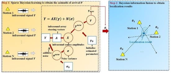
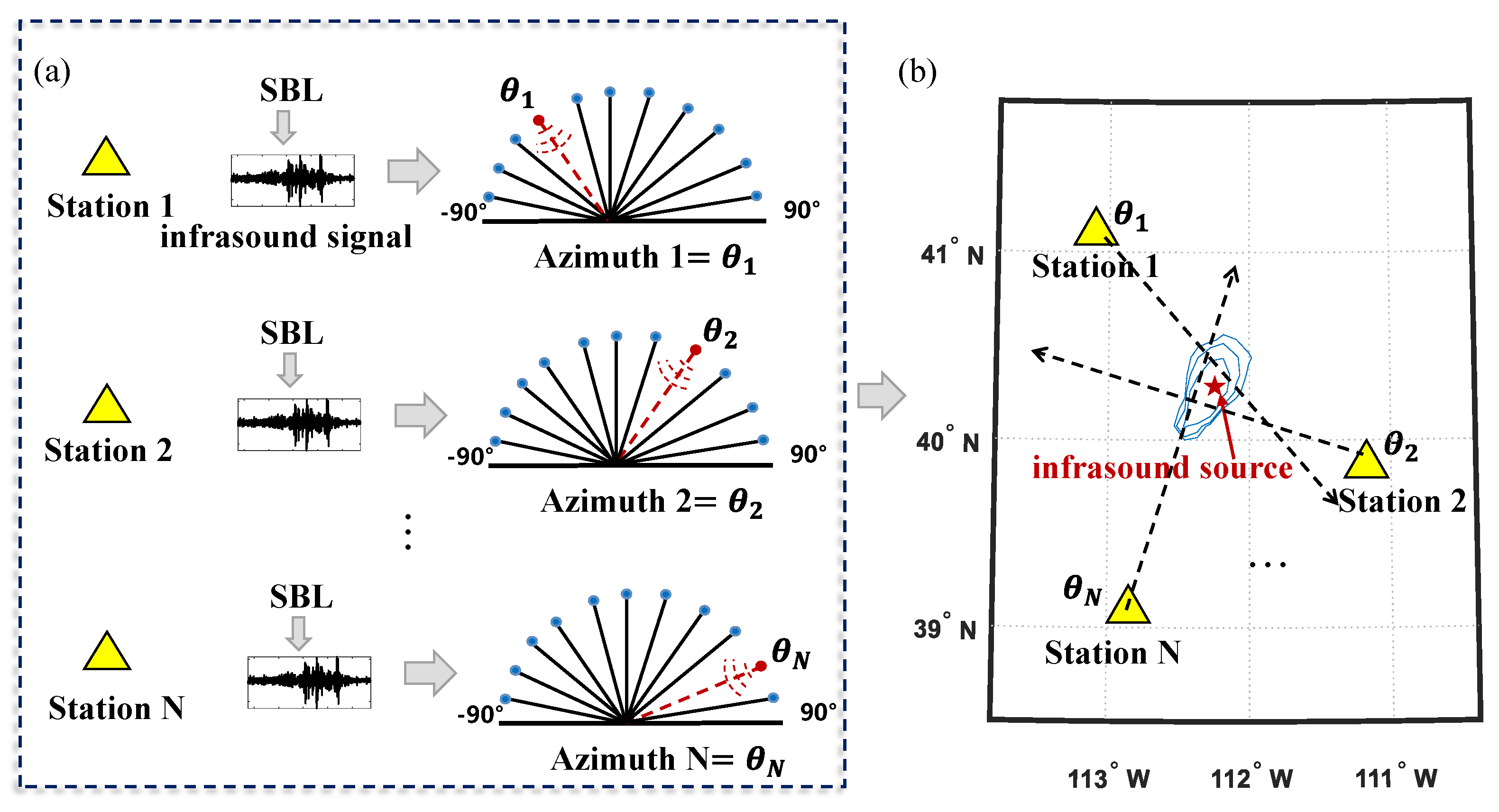
• An infrasound source localization method is developed based on the SBL algorithm under the plane wave assumption of infrasound propagation.
• The arrival azimuth estimation results, the uncertainty of the infrasound propagation environment, and the uncertainty of the measurement equipment are fused by the Bayesian information fusion algorithm to obtain the localization, making the infrasound source localization results robust to the actual atmosphere and measurement environment.
• The validity and feasibility of the proposed method are verified using a rocket motor explosion at the Utah Test and Training Range (UTTR).

The rest of this paper is organized as follows. In Section 2.1, The tau-p model for the infrasound propagation and problem statement is given. In Section 2.2, the method for estimating the arrival azimuth of infrasound sources by one arrayed station based on sources by one arrayed station based on the SBL algorithm is introduced. In Section 2.3, the Bayesian information fusion for infrasound source localization by using multiple stations is introduced. In Section 2.4, the technical flowchart for the infrasound source localization algorithm is introduced. In Section 3, the validity and feasibility of the algorithm are verified using measured infrasound data. The SBL algorithm is compared with the conventional infrasound arrival azimuth estimation algorithm. In Section 4, the availability of the proposed infrasound source localization algorithm is discussed.

2. Materials and Methods

2.1. The Tau-p Model for the Infrasound Propagation and Problem Statement

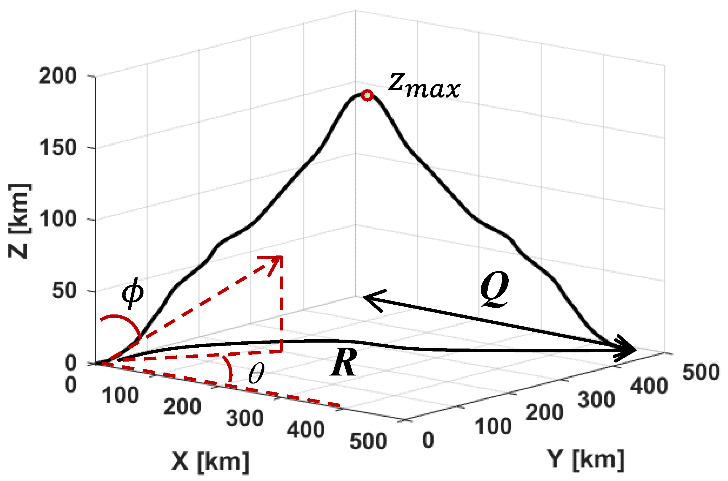
2.1.1. The Tau-p Model for the Infrasound Propagation

The tau-p model [18,20] is commonly used to simulate the trajectory of infrasound propagation in the atmosphere. It is a forward model of infasound propagation, which is suitable for visualizing the process of infrasound propagation. The principle of tau-p model is as follows.

The ray parameter p in tau-p model is

$$p=\frac{sin\left(\varphi \right)}{c_0}{\left(1+\frac{sin\left(\varphi \right)u_0}{c_0}\right)}^{-1},$$

(1)

where (1) $c_0$ is the static sound velocity at the receiving point, (2) $u_0$ is the horizontal wind speed along the infrasound propagation direction at the receiving point, and (3) $\varphi$ is the elevation angle of the emission.

The range along the ray direction in a phase loop is R. The characteristic function is $\psi$, which is formulated as

$$R(z,p)=2{\int }_{z_0}^{z\left(p\right)}\psi (z,p)\left[\frac{p}{(1-u(z\left)p\right)}+\frac{u\left(z\right)}{c{\left(z\right)}^2}\right]dz,$$

(2)

$$\psi (z,p)={\left[\frac{1}{c{\left(z\right)}^2}-\frac{p^2}{{(1-u\left(z\right)p)}^2}\right]}^{-1/2},$$

(3)

where (1) $z_0$ is lower limit of the integration (usually zero or the surface height of the infrasound source); (2) $z\left(p\right)$ is the upper limit of the integration, i.e., the maximum height of the infrasound propagation; (3) $\psi (z,p)$ is the characteristic function for which the maximum height $z_{max}$ of the infrasound trajectory can be obtained by rooting the function; (4) $c\left(z\right)=\sqrt{\frac{\gamma kT}{m}}$ is the adiabatic sound speed; and (5) $u\left(z\right)$ is the horizontal wind speed along the propagation direction.

The transverse offset Q of the infrasound propagation model is

$$Q(z,p)={\int }_{z_o}^{z\left(p\right)}\frac{1}{c{\left(z\right)}^2}\psi (z,p)v\left(z\right)dz,$$

(4)

where $v\left(z\right)$ represents the horizontal wind speed in the vertical propagation direction, and the root of $\psi (z,p)$ represents the turning point of the propagating sound line.

The diagram of the infrasound propagation model is shown in Figure 1. The infrasound propagation model is derived from the classical Wentzel–Kramers–Brillouin ($\mathrm{WKB}$) sound line theory, which suggests that the sound line will turn when the horizontal phase velocity $V_{\theta }$ matches the background effective sound velocity $c\left(z\right)+u\left(z\right)$. The propagation trajectory of the tau-p model in a phase loop is shown in Figure 1. The tau-p is a forward model, which is not applicable to the infrasound source localization problem. For this reason, infrasound is assumed to be a plane wave in the following. The infrasound source localization problem is only concerned with the source of infrasound, not with the propagation trajectory of infrasound.

2.1.2. Problem Statement for the Infrasound Source Localization

The arrival azimuth information of infrasound can be obtained from a single infrasound station, while the location information of the infrasound source is not available. From the above tau-p model, it can be seen that the accuracy of the arrival azimuth estimation of a single station is difficult to be guaranteed due to the complexity of infrasound propagation. The arrival azimuth estimation results of individual infrasound stations greatly influence the final infrasound localization results. Accurate arrival azimuth estimations are the basis for the subsequent fusion of information from multiple infrasound stations to obtain accurate infrasound source localization results.

In addition, the infrasound stations are usually distributed in the field. The localization error of the infrasound source is also affected by the uncertainty of the infrasound propagation environment and the uncertainty of the infrasound measurement equipment.

2.2. Estimating the Arrival Azimuth of Infrasound Source Based on the SBL Algorithm

The infrasound forward propagation model, i.e., the tau-p model, is introduced in Section 2.1. The trajectory of infrasound propagation can be visualized by this model. However, this model is not applicable to the arrival azimuth estimation algorithm of infrasound sources. A plane wave assumption is adopted for infrasound waves due to the ultralong distance propagation of infrasound waves, and a signal model for infrasound propagation is constructed. The infrasound source localization algorithm based on the SBL algorithm is proposed on the basis of the constructed signal model of infrasound propagation.

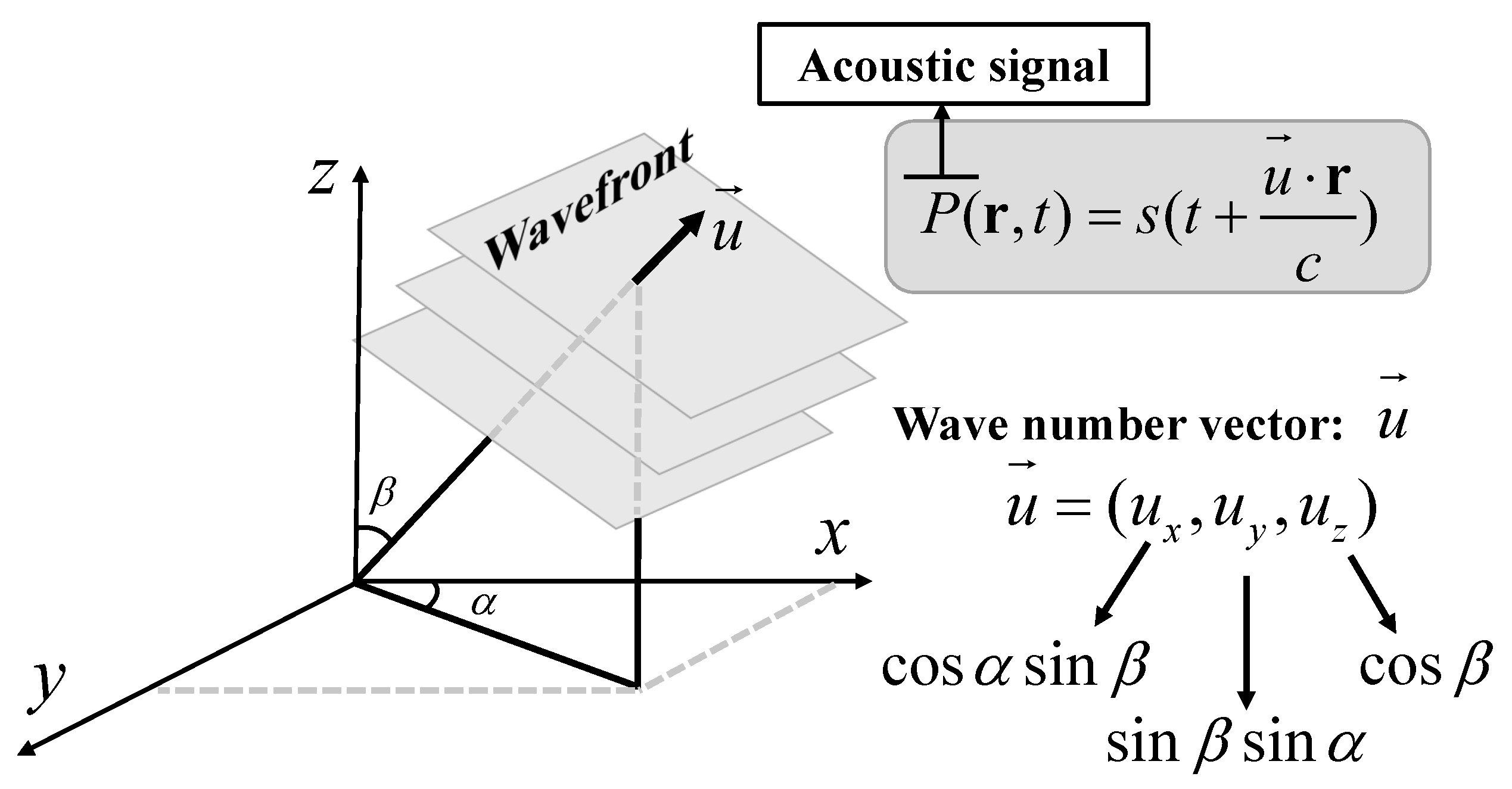
2.2.1. Signal Model for Arrival Azimuth Estimation Based on Plane Wave Assumption

It is difficult to infer the infrasound source signal from the measured signal of the infrasound station and thus obtain the arrival azimuth of the infrasound source. The above problem can be solved by building the signal model in the Equation (5) to obtain the infrasound source arrival azimuth estimation results. In this model, infrasound is assumed to be a plane wave due to the far-field propagation characteristics of infrasound in the atmosphere. The schematic diagram of three-dimensional infrasound propagation under the assumption of plane waves is shown in Figure 2. P is the acoustic signal when the initial time is t and the propagation distance is $\mathbf{r}$. The horizontal azimuth information $\alpha$ is contained in the unit normal to the wavefront $\overrightarrow{u}$.

The infrasound source signal in Equation (5) is linked to the infrasound measurement signal by the signal model through a linear regression model. The measured infrasound signal is Fourier transformed to obtain a multi-snapshot of the measured data $\mathit{Y}=\left[{\mathit{y}}_1,\dots ,{\mathit{y}}_L\right]\in {\mathbb{C}}^{N\times L}$ (N is the number of infrasound sensor and L is the number of snapshots) since the infrasound signal monitored by the infrasound station is a non-smooth signal. Large time windows of infrasound signals can be processed by this infrasound source localization algorithm using a multi-snapshot approach.

$$\mathit{Y}=\mathit{A}\mathit{X}+\mathit{N},$$

(5)

where $\mathit{X}=\left[{\mathit{x}}_1,\dots ,{\mathit{x}}_L\right]\in {\mathbb{C}}^{M\times L}$ are the actual infrasound source amplitudes and $x_{ml}$ denotes the infrasound source amplitude at the m-th discretization angle under the plane wave assumption (e.g., ${\theta }_m=-{90}^{\circ }+\frac{m-1}{M}{180}^{\circ }$) and at the l-th snapshot; M is the number of discretizations in the plane of the infrasound incoming wave direction (the plane ranges from [−90°, 90°]) discretized by the angular resolution $\Delta \theta$; and $\mathit{N}=\left[{\mathbf{n}}_1,\dots ,{\mathbf{n}}_L\right]\in {\mathbb{C}}^{N\times L}$ is additive noise, which is independent across the infrasound sensors and snapshots L. The additive noise $\mathit{N}$ of each infrasound sensor is assumed to follow a zero-averaged circularly symmetric complex Gaussian. $\mathit{A}=\left[{\mathit{a}}_1,\dots ,{\mathit{a}}_M\right]\in {\mathbb{C}}^{N\times M}$ is the transfer matrix connecting the infrasound station and the infrasound source. The infrasound array steering vectors ${\mathit{a}}_m$ are contained in the transfer matrix for all hypothetical arrival azimuths of infrasound as columns. The form of ${\mathit{a}}_m$ is as follows:

$${\mathit{a}}_m={\left[1,e^{j2\pi \frac{d}{\lambda }sin\left({\theta }_m\right)},\dots ,e^{j2\pi \frac{(N-1)d}{\lambda }sin\left({\theta }_m\right)}\right]}^T\mathrm{for}m=1,2,\dots M,$$

(6)

where d is the infrasound array aperture; $\lambda$ is the infrasound wavelength; and ${\theta }_m$ is the m-th discretized angle. The infrasound signal model is constructed under the following assumptions: (1) the infrasound source vector ${\mathit{x}}_l$ and the additive noise ${\mathbf{n}}_l$ are independent for the l-th snapshot; and (2) the noise ${\mathbf{n}}_l$ and the infrasound source vector ${\mathbf{x}}_l$ are assumed to be Gaussian, independently and identically distributed across all snapshots for $l=1,\dots ,L$.

Solving Equation (5) is an underdetermined problem due to the relationship between M and N as $M\gg N$. The infrasound source vector ${\mathit{x}}_l$ is K-sparse (K denotes the number of infrasound sources), usually $K\ll M$. The l-th activity set is defined as

$${\mathcal{M}}_l=\left\{m\in \mathbb{N}\mid x_{ml}\ne 0\right\}.$$

(7)

and ${\mathcal{M}}_l=\mathcal{M}=\left\{m_1,\dots ,m_K\right\}$ is assumed to be constant throughout the snapshot l. ${\mathit{A}}_{\mathcal{M}}\in {\mathbb{C}}^{N\times K}$ is defined to contain only the K “active” columns of $\mathit{A}$, i.e., the arrival azimuth corresponding to the index of the K non-zero values is the arrival azimuth of the infrasound signal source.

The arrival azimuth estimation of the infrasound source $\mathit{X}$ from the infrasound measurement signal $\mathit{Y}$ is a very challenging problem for Equation (5). The existence, uniqueness, and stability of the solution of Equation (5) are difficult to guarantee since Equation (5) is underdetermined. The following part of sparse Bayesian learning is introduced in Section 2.2.2 to solve this underdetermined problem so that the arrival azimuth of the infrasound source is obtained.

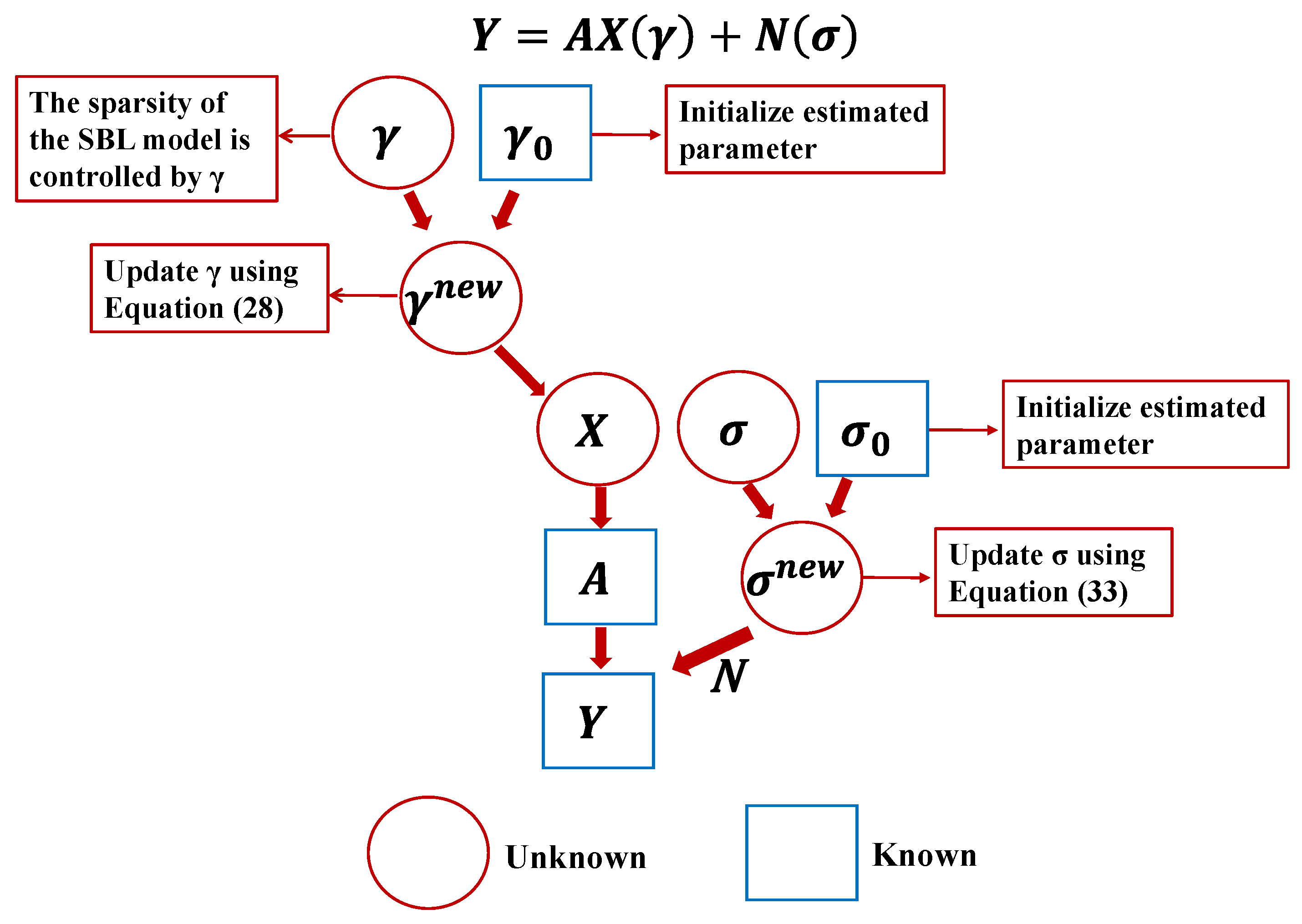
2.2.2. The SBL Algorithm for Infrasound Source Arrival Azimuth Estimation

The Bayesian formulation is used to solve linear problems (Equation (5)). The estimated parameters are considered variables of some prior distribution by the SBL algorithm. Then, this prior distribution is determined using the available knowledge. Finally, the posterior probabilities of the unknown parameters are inferred accordingly by the Bayesian rule.

(1)

Stochastic likelihood for the SBL algorithm

The additive noise in the Equation (5) is assumed to be a complex Gaussian data likelihood. The likelihood can then be written as

$$\left[\mathit{Y}\mid \mathit{X};{\sigma }^2\right]=\frac{exp\left(-\frac{1}{{\sigma }^2}{\parallel \mathit{Y}-\mathit{A}\mathit{X}\parallel }_{\mathcal{F}}^2\right)}{{\left(\pi {\sigma }^2\right)}^{NL}}.$$

(8)

(2)

Prior (prior distribution) on the infrasound sources

The complex infrasound source amplitude $x_{ml}$ is assumed to be independent in all snapshots and all discrete infrasound source arrival azimuths, and it follows a circularly symmetric complex Gaussian with zero-mean and dependent discrete infrasound source arrival azimuth variance ${\gamma }_m,m=1,\dots ,M$,

$$\left[x_{ml};{\gamma }_m\right]=\left\{\begin{array}{cc}\delta \left(x_{ml}\right),\hfill & \mathrm{for}{\gamma }_m=0\hfill \\ \frac{1}{\pi {\gamma }_m}{\mathrm{e}}^{-{\left|x_{ml}\right|}^2/{\gamma }_m},\hfill & \mathrm{for}{\gamma }_m>0\hfill \end{array}\right.,$$

(9)

$$[\mathit{X};\gamma ]=\prod _{l=1}^L\prod _{m=1}^M\left[x_{ml};{\gamma }_m\right]=\prod _{l=1}^L{\mathcal{N}}_{\mathbb{C}}(x_{ml};\mathbf{0},\mathrm{\Gamma }),$$

(10)

where ${\mathcal{N}}_{\mathbb{C}}$ is the normal distribution sign, and the unknown covariance matrix $\mathbf{\Gamma }$ for the infrasound source vector ${\mathit{x}}_l$ is assumed to be diagonal

$$\mathbf{\Gamma }=diag\left(\gamma \right),\gamma =\left[{\gamma }_1,\dots ,{\gamma }_M\right].$$

(11)

The infrasound source power is denoted as a diagonal element of $\mathbf{\Gamma }$, i.e., the hyperparameter $\gamma \ge \mathbf{0}$. The variance ${\gamma }_m\ge \mathbf{0}$ means that the arrival azimuth of this discrete infrasound source has an infrasound signal. When the variance ${\gamma }_m=0$, then $x_{ml}=0$ with probability 1. Therefore, the sparsity of the model (Equation (5)) is controlled with the hyperparameters $\gamma$, as $rank\left(\mathbf{\Gamma }\right)=K\le M$ and the covariance $\mathbf{\Gamma }$ is estimated finally by the SBL algorithm.

(3)

Posterior (posterior distribution) on the infrasound sources

The posterior probability density function is solved by the Bayesian formula on the basis of the likelihood and prior

$$\left[\mathit{X}\mid \mathit{Y};\gamma ,{\sigma }^2\right]\equiv \frac{\left[\mathit{Y}\mid \mathit{X};{\sigma }^2\right][\mathit{X};\gamma ]}{\left[\mathit{Y};\gamma ,{\sigma }^2\right]},$$

(12)

where $\left[\mathit{Y};\gamma ,{\sigma }^2\right]$ is the evidence term, which can be ignored because for a given $\gamma ,{\sigma }^2$, which is the normalization factor. Thus, Equation (12) can be simplified to

$$\left[\mathit{X}\mid \mathit{Y};\gamma ,{\sigma }^2\right]\propto \left[\mathit{Y}\mid \mathit{X};{\sigma }^2\right][\mathit{X};\gamma ]$$

(13)

$$\propto \frac{{\mathrm{e}}^{-tr\left({\left(\mathit{X}-{\mathit{\mu }}_{\mathit{X}}\right)}^H{\mathbf{\Sigma }}_x^{-1}\left(\mathit{X}-{\mathit{\mu }}_{\mathit{X}}\right)\right)}}{{\left({\pi }^{N}det{\mathbf{\Sigma }}_x\right)}^L}={\mathcal{N}}_{\mathbb{C}}\left({\mathit{\mu }}_{\mathit{X}},{\mathbf{\Sigma }}_{\mathit{x}}\right).$$

(14)

where tr means trace of square matrix, and ${(·)}^H$ means Hermitian transpose of the matrix. Their product Equation (13) is a Gaussian distribution with mean ${\mathit{\mu }}_X$ in Equation (15) and covariance ${\mathbf{\Sigma }}_{\mathit{x}}$ in Equation (16) since both the likelihood Equation (8) and the prior in Equation (10) are Gaussian distributions.

$${\mathit{\mu }}_{\mathit{X}}=\mathrm{E}\left\{\mathit{X}\mid \mathit{Y};\gamma ,{\sigma }^2\right\}=\mathbf{\Gamma }{\mathit{A}}^H{\mathbf{\Sigma }}_{\mathit{y}}^{-1}\mathit{Y},$$

(15)

$${\mathbf{\Sigma }}_{\mathit{x}}=\mathrm{E}\left\{\left({\mathit{x}}_l-{\mathit{\mu }}_{{\mathit{x}}_l}\right){\left({\mathit{x}}_l-{\mathit{\mu }}_{{\mathit{x}}_l}\right)}^H\mid \mathit{Y};\gamma ,{\sigma }^2\right\}=\mathbf{\Gamma }-\mathbf{\Gamma }{\mathit{A}}^H{\mathbf{\Sigma }}_{\mathit{y}}^{-1}\mathit{A}\mathbf{\Gamma },$$

(16)

where the infrasound sensor data covariance ${\mathbf{\Sigma }}_{\mathit{y}}$

$$\begin{array}{cc}\hfill {\mathbf{\Sigma }}_{\mathit{y}}& =\mathrm{E}\left\{{\mathit{y}}_l{\mathit{y}}_l^H\right\}={\sigma }^2{\mathit{I}}_N+\mathit{A}\mathbf{\Gamma }{\mathit{A}}^H\hfill \end{array},$$

(17)

$$\begin{array}{cc}\hfill {\mathbf{\Sigma }}_{\mathit{y}}^{-1}& ={\sigma }^{-2}{\mathit{I}}_N-{\sigma }^{-2}\mathit{A}{\left(\frac{1}{{\sigma }^2}{\mathit{A}}^H\mathit{A}+{\mathbf{\Gamma }}^{-1}\right)}^{-1}{\mathit{A}}^H{\sigma }^{-2}\hfill \\ \hfill & ={\sigma }^{-2}{\mathit{I}}_N-{\sigma }^{-2}\mathit{A}{\mathbf{\Sigma }}_{\mathit{x}}{\mathit{A}}^H{\sigma }^{-2}\hfill \end{array}$$

(18)

where ${\mathrm{I}}_N$ is the identity matrix of order N and E means expected value. The posterior mean ${\widehat{\mathit{X}}}^{\mathrm{MAP}}$ can be obtained using the maximum a posteriori (MAP) method when $\gamma$ and ${\sigma }^2$ are known.

$${\widehat{\mathit{X}}}^{\mathrm{MAP}}=\mathbf{\Gamma }{\mathit{A}}^H{\mathbf{\Sigma }}_{\mathit{y}}^{-1}\mathit{Y}={\mathit{\mu }}_{\mathit{X}}.$$

(19)

(4)

Evidence on the infrasound sources

The $\gamma$ and ${\sigma }^2$ in the Equations (16)–(19) are considered as hyperparameters. They are estimated by maximizing the evidence. The evidence that is considered as a constant in Equation (12) is the product of the integration of the likelihood part in the Equation (8) and the prior part in the Equation (10) over the complex infrasound source amplitude $\mathit{X}$.

$$\left[\mathit{Y};\gamma ,{\sigma }^2\right]=\prod _{l=1}^L{\mathcal{N}}_{\mathbb{C}}\left({\mathit{y}}_l;\mathbf{0},{\mathbf{\Sigma }}_{{\mathit{y}}_l}\right)={\int }_{{\mathbb{R}}^{2ML}}\left[\mathit{Y}\mid \mathit{X};{\sigma }^2\right][\mathit{X};\gamma ]\mathrm{d}\mathit{X},$$

(20)

The logarithm of the evidence is

$$\begin{array}{cc}\hfill log\left[\mathit{Y};\gamma ,{\sigma }^2\right]& \propto -\sum _{l=1}^L\left({\mathit{y}}_l^H{\mathbf{\Sigma }}_{{\mathit{y}}_l}^{-1}{\mathit{y}}_l+logdet{\mathbf{\Sigma }}_{{\mathit{y}}_l}\right),\hfill \end{array}$$

(21)

where the infrasound array data sample covariance matrix (SCM) is defined by the following equation

$${\mathit{S}}_{\mathit{y}}=\mathit{Y}{\mathit{Y}}^H/L.$$

(22)

(5)

Infrasound source power estimation using the SBL algorithm

The above is the Bayesian statistical modeling phase, and the following is the solution phase. The infrasound source power (i.e., ${\gamma }_m$) was estimated by the SBL algorithm following the type-II maximum likelihood (maximizing the evidence) in Equation (23) [14]. The hyperparameters $\widehat{\gamma }$ and ${\widehat{\sigma }}^2$ can be obtained by the type-II maximum likelihood (maximizing the evidence). That is, the following equation:

$$\left[\widehat{\gamma },{\widehat{\sigma }}^2\right]=\underset{\gamma \ge 0,{\sigma }^2>0}{argmax}log\left[\mathit{Y};\gamma ,{\sigma }^2\right],$$

(23)

where $argmax$ is an abbreviation for “arguments of the maxima”. The objective function in Equation (23) is differentiated to obtain a local maximum. The following are derivative relations:

$$\frac{\partial {\mathbf{\Sigma }}_{{\mathit{y}}_l}^{-1}}{\partial {\gamma }_m}=-{\mathbf{\Sigma }}_{{\mathit{y}}_l}^{-1}\frac{\partial {\mathbf{\Sigma }}_{{\mathit{y}}_l}}{\partial {\gamma }_m}{\mathbf{\Sigma }}_{{\mathit{y}}_l}^{-1}=-{\mathbf{\Sigma }}_{{\mathit{y}}_l}^{-1}{\mathit{a}}_m{\mathit{a}}_m^H{\mathbf{\Sigma }}_{{\mathit{y}}_l}^{-1},$$

(24)

$$\frac{\partial logdet\left({\mathbf{\Sigma }}_{{\mathit{y}}_l}\right)}{\partial {\gamma }_m}=tr\left[{\mathbf{\Sigma }}_{{\mathit{y}}_l}^{-1}\frac{\partial {\mathbf{\Sigma }}_{{\mathit{y}}_l}}{\partial {\gamma }_m}\right]={\mathit{a}}_m^H{\mathbf{\Sigma }}_{{\mathit{y}}_l}^{-1}{\mathit{a}}_m,$$

(25)

the derivative of Equation (21) is

$$\begin{array}{cc}\hfill \frac{\partial logp\left(\mathit{Y};\gamma ,{\sigma }^2\right)}{\partial {\gamma }_m}& =\sum _{l=1}^L\left({\mathit{y}}_l^H{\mathbf{\Sigma }}_{{\mathit{y}}_l}^{-1}{\mathit{a}}_m{\mathit{a}}_m^H{\mathbf{\Sigma }}_{{\mathit{y}}_l}^{-1}{\mathit{y}}_l-{\mathit{a}}_m^H{\mathbf{\Sigma }}_{{\mathit{y}}_l}^{-1}{\mathit{a}}_m\right)\hfill \\ & =\sum _{l=1}^L{\left|{\mathit{y}}_l^H{\mathbf{\Sigma }}_{{\mathit{y}}_l}^{-1}{\mathit{a}}_m\right|}^2-\sum _{l=1}^L{\mathit{a}}_m^H{\mathbf{\Sigma }}_{{\mathit{y}}_l}^{-1}{\mathit{a}}_m.\hfill \end{array}$$

(26)

For the solution to Equation (21), the necessary conditions are set, i.e., $\frac{\partial log p\left(\mathit{Y};\gamma ,{\sigma }^2\right)}{\partial {\gamma }_m}=0$. To obtain an iterative equation in ${\gamma }_m$, the first term in the Equation (26) is multiplied by the factor $\left(\frac{{\gamma }_m^{\mathrm{old}}}{{\gamma }_m^{\mathrm{new}}}\right)$, whereby

$$\left(\frac{{\gamma }_m^{\mathrm{old}}}{{\gamma }_m^{\mathrm{new}}}\right)\sum _{l=1}^L{\left|{\mathit{y}}_l^H{\mathbf{\Sigma }}_{{\mathit{y}}_l}^{-1}{\mathit{a}}_m\right|}^2-\sum _{l=1}^L{\mathit{a}}_m^H{\mathbf{\Sigma }}_{{\mathit{y}}_l}^{-1}{\mathit{a}}_m=0.$$

(27)

Assuming ${\gamma }_m^{\mathrm{old}}$ and ${\mathbf{\Sigma }}_{{\mathit{y}}_l}$ are known from previous iteration or initialization, the fixed point iteration for ${\gamma }_m$ is obtained by rewriting Equation (27) (with similarities to [10,11,13,21]:

$${\gamma }_m^{\mathrm{new}}={\gamma }_m^{\mathrm{old}}\left(\frac{{\sum }_{l=1}^L{\left|{\mathit{y}}_l^H{\mathbf{\Sigma }}_{{\mathit{y}}_l}^{-1}{\mathit{a}}_m\right|}^2}{{\sum }_{l=1}^L{\mathit{a}}_m^H{\mathbf{\Sigma }}_{{\mathit{y}}_l}^{-1}{\mathit{a}}_m}\right).$$

(28)

Usually, the convergence of such fixed-point iterations is not guaranteed [11]. A larger number of iterations (about 1000) is required to guarantee the convergence of the iteration parameters. In this paper, the maximum number of iterations of the parameter $\gamma$ is set to 1000.

(6)

Infrasound source noise variance estimation (hyperparameter ${\sigma }^2$)

The noise is also a part of the model (Equation (5)) because, in the SBL algorithm, the sharpness of the local maxima in the $\gamma$ spectrum is controlled by the noise variance, i.e., the higher the noise level, the wider the peaks in the $\gamma$ spectrum. By maximizing the evidence-based approach, similar to the approach used to estimate the $\gamma$, one can estimate the infasound source noise variance $\sigma$ [16,22]. The sparsity of the matrix ${\widehat{\mathit{X}}}^{\mathrm{MAP}}$ is controlled by $\mathbf{\Gamma }$. Thus, the active set $\mathcal{M}$ is defined as

$$\mathcal{M}=\left\{m\in \mathbb{N}\mid {\gamma }_m>0\right\}.$$

(29)

The infrasound sensors data covariance matrix is

$${\mathbf{\Sigma }}_{\mathit{y}}={\mathbf{\Sigma }}_{{\mathit{n}}_l}+{\mathit{A}}_{\mathcal{M}}{\mathbf{\Gamma }}_{\mathcal{M}}{\mathit{A}}_{\mathcal{M}}^H,$$

(30)

where ${\mathbf{\Sigma }}_{{\mathbf{n}}_l}={\sigma }^2{\mathit{I}}_N$; ${\mathit{A}}_{\mathcal{M}}$ is the active infrasound array steering vectors and it consists of K columns of $\mathit{A}$, indexed by $\mathcal{M}$; the set $\mathcal{M}$ denotes the position of $\gamma$ non-zero entries with cardinality K, and it is estimated by selecting the strongest K peak from ${\widehat{\gamma }}^{\mathrm{new}}$; and ${\mathbf{\Gamma }}_{\mathcal{M}}=diag\left({\gamma }_{\mathcal{M}}^{\mathrm{new}}\right)$ is the covariance matrix of the K active infrasound sources. The Jaffer’s necessary condition at the optimal solution $\left({\mathbf{\Gamma }}_{\mathcal{M}},{\sigma }^2\right)$ must be satisfied, i.e., the following relationship is satisfied:

$${\mathit{A}}_{\mathcal{M}}^H\left({\mathit{S}}_{\mathit{y}}-{\mathbf{\Sigma }}_{\mathit{y}}\right){\mathit{A}}_{\mathcal{M}}=\mathbf{0},$$

(31)

where $S_y$ is the infrasound array data sample covariance matrix. The necessary condition of Jaffer is satisfied since arbitrary correlations between infrasound source signals are allowed. Substituting Equation (30) into Equation (31) gives

$${\mathit{A}}_{\mathcal{M}}^H\left({\mathit{S}}_{\mathit{y}}-{\mathbf{\Sigma }}_{{\mathbf{n}}_l}\right){\mathit{A}}_{\mathcal{M}}={\mathit{A}}_{\mathcal{M}}^H{\mathit{A}}_{\mathcal{M}}{\mathbf{\Gamma }}_{\mathcal{M}}{\mathit{A}}_{\mathcal{M}}^H{\mathit{A}}_{\mathcal{M}},$$

(32)

multiplying (32) from right and left with the ${\mathit{A}}_{\mathcal{M}}^{+}={\left({\tilde{A}}_{\mathcal{M}}^{\dot{H}}{\mathit{A}}_{\mathcal{M}}\right)}^{-1}{\mathit{A}}_{\mathcal{M}}^H$ and ${\mathit{A}}_{\mathcal{M}}^{+H}$, respectively, and subtracting $S_y$ from both sides yields [22]. The ${\sigma }^2$ estimate of the infrasound source noise variance is

$${\left({\sigma }^2\right)}^{\mathrm{new}}=\frac{1}{N-K}tr\left(\left({\mathit{I}}_N-{\mathit{A}}_{\mathcal{M}}{\mathit{A}}_{\mathcal{M}}^{+}\right){\mathit{S}}_{\mathit{y}}\right).$$

(33)

2.2.3. The Pseudocode for the SBL-Based Estimation Algorithm for Infrasound Arrival Azimuth

The SBL-based infrasound source arrival azimuth estimation algorithm is summarized in Algorithm 1. The structure diagram of the Bayesian hierarchical model is shown in Figure 3. The ${\mathit{\mu }}_{\mathit{X}}$ in Equation (15) and ${\mathbf{\Sigma }}_{\mathit{y}}$ in Equation (17) are updated iteratively using the current $\gamma$ for a given observed infrasound sensors data $\mathit{Y}$. Then ${\gamma }_m$ for $m=1,\dots ,M$ is updated via Equation (28) and then Equation (33) is uesd to estimate the noise variance ${\sigma }^2$. The infrasound source is assumed to be single in this paper, assuming that only one infrasound event occurs at a given moment, i.e., $K=1$, for estimating the noise variance in the Equation (33). The algorithm performance was not found to be sensitive to the number of infrasound sources K in the simulations. The algorithm is made more flexible by this assumption since there is no need to know the true number of infrasound sources. The relative improvement in the total infrasound source power is measured by the convergence rate $ϵ$ in the Equation (34), where ${\parallel ·\parallel }_1$ is the 1 norm. The algorithm stops when $ϵ\le {ϵ}_{min}$. In this paper, the ${ϵ}_{min}$ is set to ${10}^{-4}$. The $j_{max}$ is the maximum number of iterations. In this paper, the $j_{max}$ is set to 1000. The output is the active set $\mathcal{M}$ in the Equation (29). The estimated value of the arrival azimuth $\theta$ is the angle corresponding to the maximum gamma value ${\gamma }_{max}$.

$$ϵ={∥{\gamma }_m^{\mathrm{new}}-{\gamma }_m^{\mathrm{old}}∥}_1/{∥{\gamma }_m^{\mathrm{old}}∥}_1,$$

(34)

Algorithm 1: The SBL-based infrasound source orientation algorithm

Input:$\mathit{A}\in {\mathbb{C}}^{N\times M},\mathit{Y}\in {\mathbb{C}}^{N\times L},K=1,{\sigma }_0^2=0.1,{\gamma }_0=1,{ϵ}_{min}={10}^{-4},j_{max}=1000$;

Output:${\gamma }^{\mathrm{new}},{\left({\sigma }^2\right)}^{\mathrm{new}}$, $\theta$;

1: initialize: $j=0,{\sigma }^2={\sigma }_0^2,\gamma ={\gamma }_0$;

2: while $\left(ϵ>{ϵ}_{min}\right)\mathrm{and}\left(j<j_{max}\right)$;

3:       Compute: ${\mathbf{\Sigma }}_{\mathbf{y}}={\sigma }^2{\mathit{I}}_N+\mathit{A}\mathbf{\Gamma }{\mathit{A}}^H$

4:       Compute: ${\mathbf{\mu }}_m={\gamma }_m{\mathit{a}}_m^H{\mathbf{\Sigma }}_{\mathbf{y}}^{-1}\mathit{Y}$

5:       ${\gamma }_m^{\mathrm{new}}\mathrm{update}\mathrm{for}\forall m\mathrm{using}\mathrm{Equation}\left(28\right)$

6:       ${\left({\sigma }^2\right)}^{\mathrm{new}}=\frac{1}{N-K}tr\left(\left({\mathit{I}}_N-{\mathit{A}}_{\mathcal{M}}{\mathit{A}}_{\mathcal{M}}^{+}\right){\mathbf{S}}_{\mathbf{y}}\right)$

7:       $ϵ={∥{\gamma }^{\mathrm{new}}-{\gamma }^{\mathrm{old}}∥}_1/{∥{\gamma }^{\mathrm{old}}∥}_1$

8:       $\theta$ is the angle corresponding to ${\gamma }_{max}$

9: end

2.3. Bayesian Information Fusion for Infrasound Source Localization

The arrival azimuth estimation results of individual infrasound stations can be derived from the SBL algorithm, and the accuracy of infrasound source localization can be greatly improved when the fusion of information from infrasound stations is considered. Multiple information is fused by the Bayesian information fusion algorithm based on Bayesian formulation [23,24]. In this paper, the azimuth, measurement error, and model error of the infrasound station are combined by a Bayesian information fusion algorithm. The final fused multi-information infrasound source localization results are obtained.

2.3.1. Posteriori Distribution for Infrasound Source Localization

The arrival azimuths of the n infrasound stations estimated by the SBL algorithm are expressed as $\mathbf{\theta }=\left[{\theta }_1,\cdots ,{\theta }_n\right]$. The location of the i-th infrasound station can be represented by $\left(x_i,y_i\right)$, and this is the Cartesian coordinate system, which can be transformed from the geodetic coordinate system.

The location parameter $\mathbf{m}=\left\{x_0,y_0\right\}$ to be estimated is the candidate infrasound source location. The posterior probability density function of the location parameter is

$$[\mathbf{m}\mid \mathbf{\theta }]=c\left[\mathbf{\theta }\right]\left[\mathbf{m}\right][\mathbf{\theta }\mid \mathbf{m}],$$

(35)

where $[\mathbf{\theta }\mid \mathbf{m}]$ is the likelihood function; $c\left[\mathbf{\theta }\right]$ ensures that the likelihood function $[\mathbf{\theta }\mid \mathbf{m}]$ integrates to unity; and $\left[\mathbf{m}\right]$ is the prior for the infrasound source location parameters.

2.3.2. Likelihood Function

The likelihood function can be derived from the product of the estimated components of the arrival azimuths of all infrasound stations, under the assumption that the detections of each station are independent of each other.

$$[\mathbf{\theta }\mid \mathbf{m}]\equiv \prod _{i=1}^n{\Theta }_i\left({\theta }_i\mid \mathbf{m}\right).$$

(36)

The consistency between the observed arrival azimuth, and the selected model parameters is measured by the ${\Theta }_i$, for a given i-th infrasound station. It is assumed that the errors between the observed arrival azimuths and the selected model parameters conform to a Gaussian distribution. The arrival azimuth likelihood function measured for the ith station is

$${\Theta }_i\left({\theta }_i\mid \mathbf{m}\right)\equiv \frac{1}{\sqrt{2\pi {\sigma }_{\theta }^2}}exp\left[-\frac{1}{2}{\left(\frac{{\gamma }_i}{{\sigma }_{\theta }}\right)}^2\right].$$

(37)

Let $(x_i,y_i)$ represent the candidate infrasound source position to the i-th infrasound station, then the arrival azimuth estimation residuals are

$${\gamma }_i\equiv {\theta }_i-arctan\left(\frac{y_i-y_0}{x_i-x_0}\right).$$

(38)

The total variances in the arrival azimuth estimation are denoted ${\sigma }_{\theta }^2$, which, accounts for both infrasound measurement equipment ${\sigma }_{\theta ,\mathrm{meas}}^2$ and infrasound propagation model ${\sigma }_{\theta ,\mathrm{mod}}^2$ error contributions

$${\sigma }_{\theta }^2={\sigma }_{\theta ,\mathrm{meas}}^2+{\sigma }_{\theta ,\mathrm{mod}}^2,$$

(39)

where ${\sigma }_{\theta }^2$ can be estimated using historical infrasound events. Usually, ${\sigma }_{\theta }=3.5^{\circ }$ is suggested by an analysis of the western United States earthquakes [6]. The ${\sigma }_{\theta }=3.5^{\circ }$ is mainly determined by the combination of discretization used in the slowness plane, the array aperture, and the signal-to-noise ratio (SNR). The variance on the infrasound measurement equipment error ${\sigma }_{\theta ,\mathrm{meas}}^2$ is a function of the distance between the sensors of the infrasound station, sampling frequency, and wavelength. The variance on the infrasound propagation model error ${\sigma }_{\theta ,mod}^2$ is derived from the variation of wind speed, wind direction, and temperature.

2.3.3. The Framework for Infrasound Source Localization

An infrasound source localization algorithm for distributed stations based on the SBL algorithm and Bayesian information fusion is proposed in the context of the large-scale global distribution of infrasound stations. The accuracy of the infrasound source can be improved by the proposed algorithm while incorporating the uncertainty of the infrasound measurement equipment and the infrasound propagation uncertainty into the infrasound source localization results. First, the infrasound signals recorded at individual stations are processed based on the SBL algorithm to obtain the azimuth information of the corresponding stations. Second, infrasound propagation in the atmosphere is susceptible to wind speed, temperature, and atmospheric density, and the effect is modeled as the model variance ${\sigma }_{\theta ,\mathrm{mod}}$. Third, the measurement error generated during infrasound measurement is modeled as the measurement variance ${\sigma }_{\theta ,\mathrm{meas}}$. Finally, the Bayesian information fusion is used to fuse the localization results, model errors, and measurement errors from multiple stations to obtain the localization results of infrasound sources. The schematic diagram for Bayesian information fusion algorithm is shown in Figure 4.

2.4. Technical Flow Chart of the Proposed Infrasound Source Localization Method

The actual measured infrasound data are first used to obtain the arrival azimuth information of each station using a sparse Bayesian learning algorithm. Then, the arrival azimuth information obtained from each station is imported into the Bayesian information fusion algorithm to obtain the localization results of the infrasound source. The technical flow chart of the infrasound source localization method proposed in this paper is shown in Figure 5.

3. Results

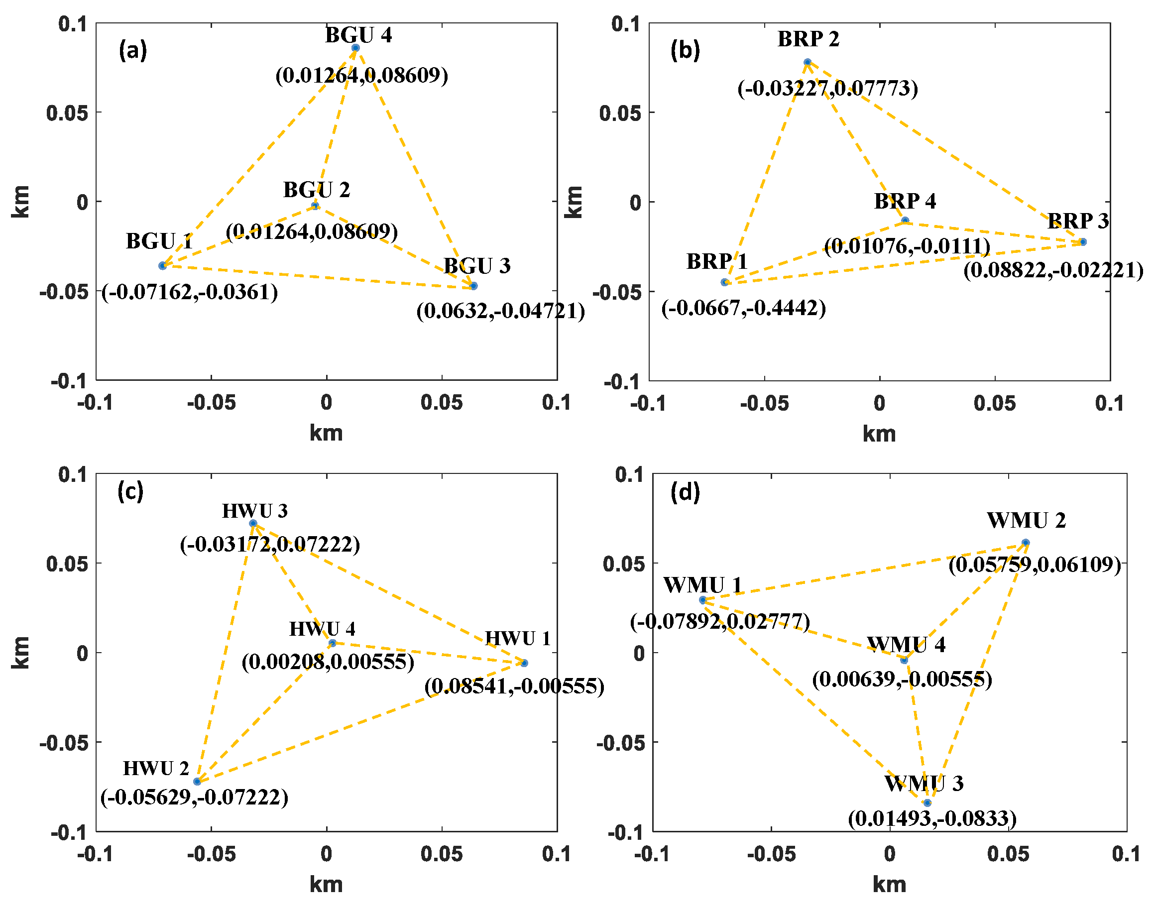
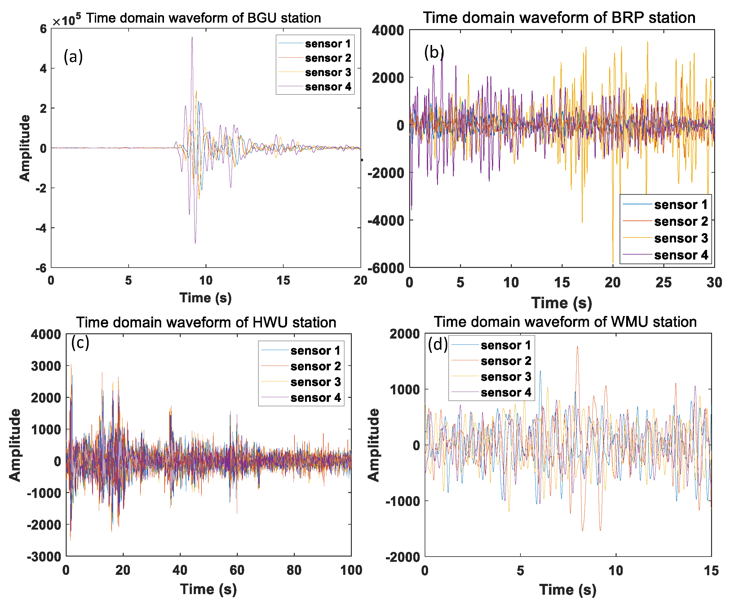
3.1. Experimetntal Setup

The SBL algorithm was tested by UTTR’s rocket motor explosion data (explosive weight 39,000 lb (approximately 17,690 kg)) [25,26,27] to verify the feasibility of the SBL algorithm. For the UTTR event, the real source location and the location information of the four observatories are shown in the

Table 1. UTTR source location and observations (See also in Figure 13).

Station	Location
Source location	41.1310°N, 112.8950°W
BGU	40.9204°N, 112.0309°W
BRP	39.4727°N, 110.7409°W
HWU	41.6071°N, 111.5652°W
WMU	40.0795°N, 111.8310°W

.

Firstly, the range of reconstruction frequency is selected according to the spectrum of infrasound. In this paper, the frequency range of 1–2 Hz is chosen for signal reconstruction, and then the reconstruction signal corresponding to each reconstruction frequency is solved at an interval of 0.1 Hz. The reconstructed signal is substituted into the SBL algorithm to solve the gamma value $\gamma$ corresponding to the reconstruction frequency. The estimated value of the arrival azimuth $\theta$ is the angle corresponding to ${\gamma }_{max}$.

The infrasound data recorded at the four stations BGU, BRP, HWU, and WMU were used as the experimental data, which were sampled at a frequency of 100 Hz. The infrasound signals with a passband of 1–5 Hz were selected using a Butterworth bandpass filter. The array structure of the four infrasound stations is shown in Figure 6.

The time-domain waveforms of the four stations are shown in Figure 7. The interception of the infrasound signals recorded at each station is selected as follows for each station. The BGU station intercepts 20 s signal as well as the sensor selections BGU1 and BGU3, and the array aperture is 135 m; the BRP station intercepts the 30 s signal as well as the sensor selections BRP1 and BRP3, and array aperture is 150 m; the HWU station intercepts the 100 s signal as well as the sensor selections HWU1 and HWU3, and the array aperture is 140 m; and the WMU station intercepts the 15 s signal as well as the sensor selections WMU2 and WMU3, and array aperture is 150 m. The intercepted infrasound is substituted into the SBL algorithm to obtain the azimuth information of the four stations. The infrasound signal and the SBL algorithm parameter setting are shown in

Table 2. Infrasound signal and the SBL algorithm parameter setting.

Station Number	Snapshots	Array Aperture	Angular Resolution	Sensor
BGU	39	135 m	0.1	BGU1, BGU3
BRP	39	150 m	0.1	BRP1, BRP3
HWU	39	140 m	0.1	HWU1, HWU3
WMU	39	150 m	0.1	WMU2, WMU3

.

The main parameters of the sparse Bayesian learning algorithm are set as follows: the number of snapshots is set to 39, the angular resolution $\Delta \theta$ is 0.1°, the convergence error ${ϵ}_{min}$ is 0.0001, the maximum number of iterations $j_{max}$ is 1000, and the sampling frequency is 100 Hz. The process of transforming the infrasound signal from the time domain to the frequency domain is shown in the Figure 8. The infrasound frequency domain signal is substituted into the sparse Bayesian learning algorithm for the solution, and the results are shown in Figure 9.

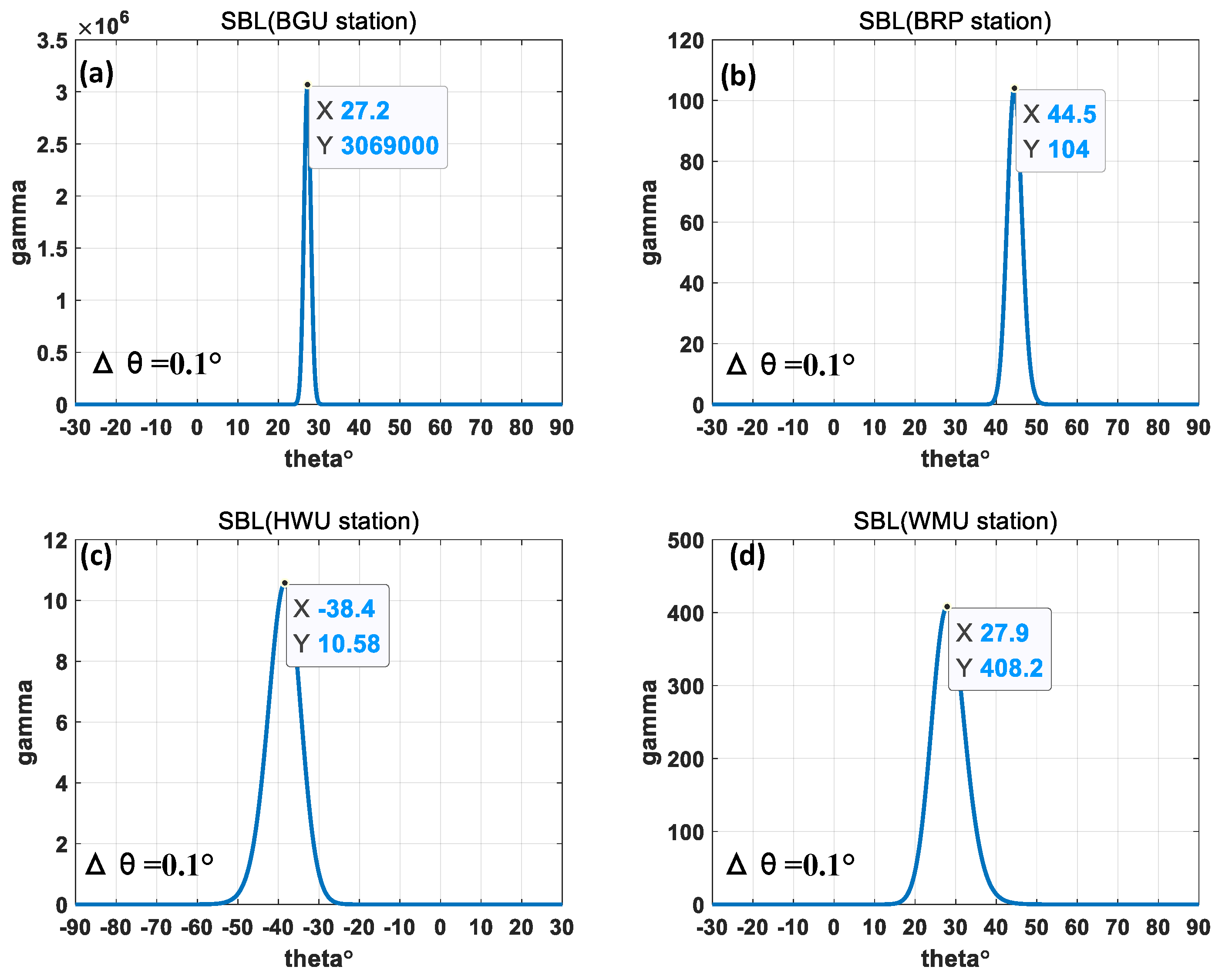
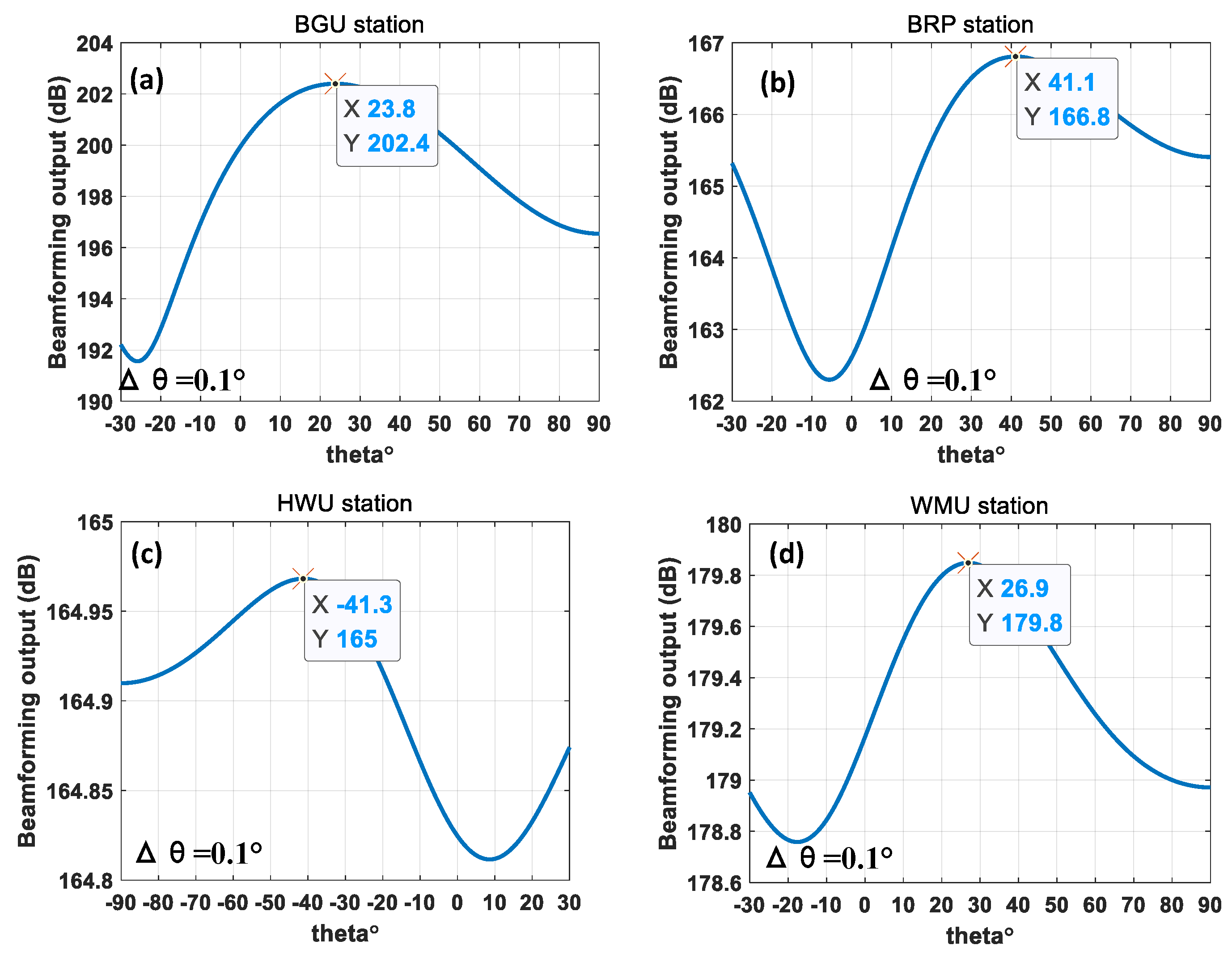
3.2. Arrival Azimuth Estimation Results

The result of the arrival azimuth estimation of the SBL algorithm is the angle value corresponding to the maximum gamma value ${\gamma }_{max}$. The results of the SBL algorithm arrival azimuth estimation $\theta$ for the four infrasound stations BGU, BRP, HWU, and WMU are 27.2°, 44.5°, −38.4°, and 27.9°, respectively, as shown in Figure 9. The arrival azimuth estimations with the SBL algorithm for the four stations were converted to azimuths in the geographic coordinate system by considering the effect of the array tilt angles of the infrasound stations, which were 4.71°, 8.15°, −33.67°, and 73.54° for the BGU, BRP, HWU, and WMU stations, respectively. The array tilt angle is defined as the acute angle between a linear array of two array sensors and the latitude line in the geographic coordinate system. The azimuths obtained by the four stations are shown in Figure 10.

It can be seen that the converted arrival azimuths of the SBL algorithm results for the four infrasound stations BGU, BRP, HWU, and WMU are 32.91°, 307.35°, 252.07°, and 314.35°, respectively. The actual azimuths between the infrasound source and the infrasound stations were compared to obtain the arrival azimuth estimation errors of the SBL algorithm, as shown in

Table 3. Arrival azimuth estimation error of the SBL algorithm for four stations.

Station Number	Arrival Azimuth Estimation Results (°)	Actual Azimuths (°)	Estimation Error (°)
BGU	32.91	31.99	0.92
BRP	307.35	307.51	0.16
HWU	252.07	250.54	1.53
WMU	314.35	314.66	0.31

.

3.3. Comparison of the Error of Arrival Azimuth Estimation between SBL Algorithm, FK Analysis, and BF Algorithm

The SBL-based arrival azimuth estimation algorithm and the conventional infrasound arrival azimuth estimation algorithm (FK analysis) are applied for comparison in terms of the accuracy of arrival azimuth estimation. The complete slowness vector of infasound in the plane-wave hypothesis can be measured by the FK analysis. Additionally, the infrasound power distribution at different slownesses is calculated by FK analysis [28,29]. For the same infrasound events, the arrival azimuth estimation results of the FK analysis are shown in Figure 11. The azimuths obtained from the FK analysis of the four stations BGU, BRP, HWU, and WMU are 29.05°, 312.13°, 247.83°, and 323.53°, respectively.

The beamforming [30] algorithm is used to process the infrasound signal for the same infrasound event. The delay-and-sum technique is utilized by the algorithm to enhance the coherent signal and suppress the non-coherent background noise to obtain the arrival azimuth information. The results of beamforming are shown in Figure 12. From Figure 12, it can be seen that the results of the beamforming algorithm for the BGU, BRP, HWU, and WMU stations are 23.8°, 14.1°, −41.3°, and 26.9°, respectively. The results of the beamforming algorithms are converted into arrival azimuths by considering the effect of array inclination. The estimated azimuth of arrival results for BGU, BRP, HWU, and WMU stations are 28.51°, 310.74°, 254.97°, and 313.36°, and the orientation errors are 3.48°, 3.23°, 4.43°, and 1.30°, respectively.

The arrival azimuth estimation errors of the three arrival azimuth estimation algorithms are shown in

Table 4. Comparison of the error of arrival azimuth estimation between SBL algorithm, FK analysis, and beamforming algorithm.

Station Number	SBL Arrival Azimuth Estimation Error (°)	FK Arrival Azimuth Estimation Error (°)	Beamforming Arrival Azimuth Estimation Error (°)
BGU	0.92	2.94	3.48
BRP	0.16	4.78	3.23
HWU	1.53	2.71	4.43
WMU	0.31	9.18	1.30

.

According to Table 4, the arrival azimuth estimation errors of all four stations of the SBL algorithm are within 2°. The error is mainly due to the influence of low-frequency noise (such as thunderstorm noise, ground noise, and the noise of the measurement station itself) during the long-distance propagation of infrasound. The superiority of the SBL algorithm over the FK analysis in terms of arrival azimuth estimation accuracy is shown in Table 4. Compared with beamforming, the estimation error of the arrival azimuth of SBL is smaller and the side flaps are smaller, as can be seen from Table 4 and Figure 12. Therefore, the arrival azimuth estimation results of the SBL algorithm are used as prior knowledge for the Bayesian information fusion algorithm to perform fusion localization in the following.

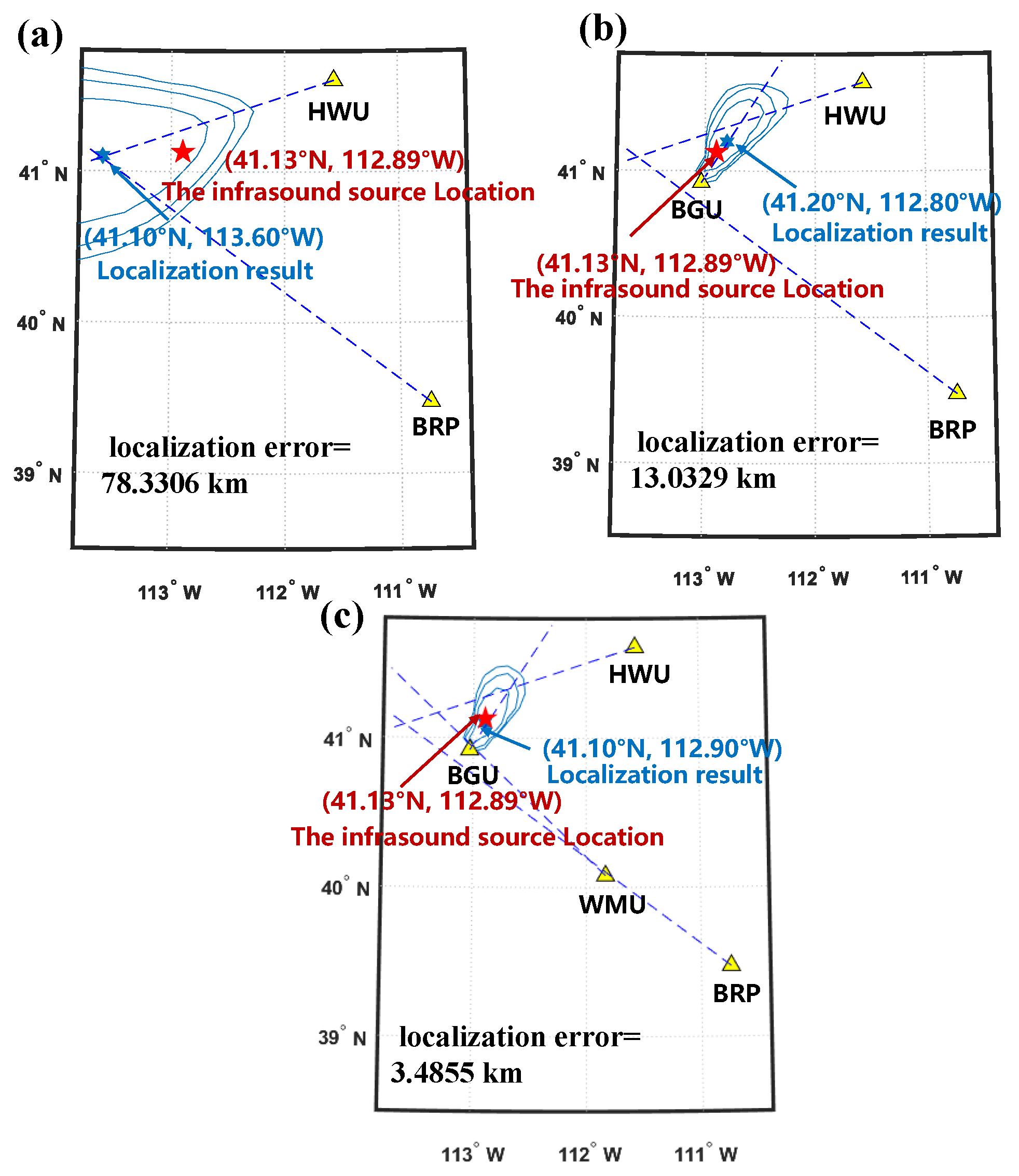
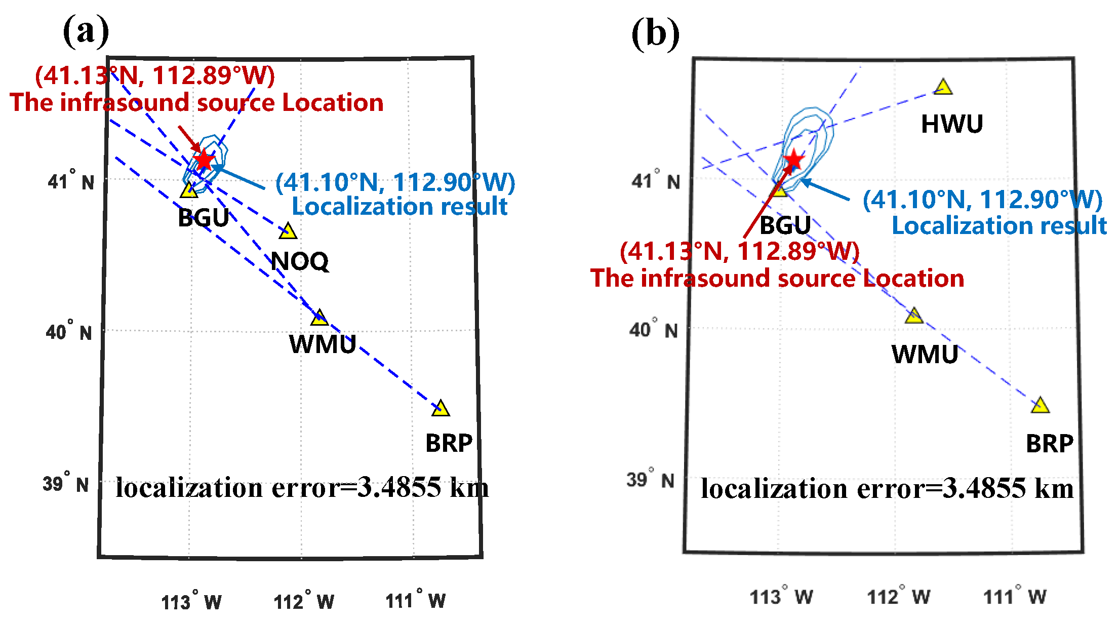
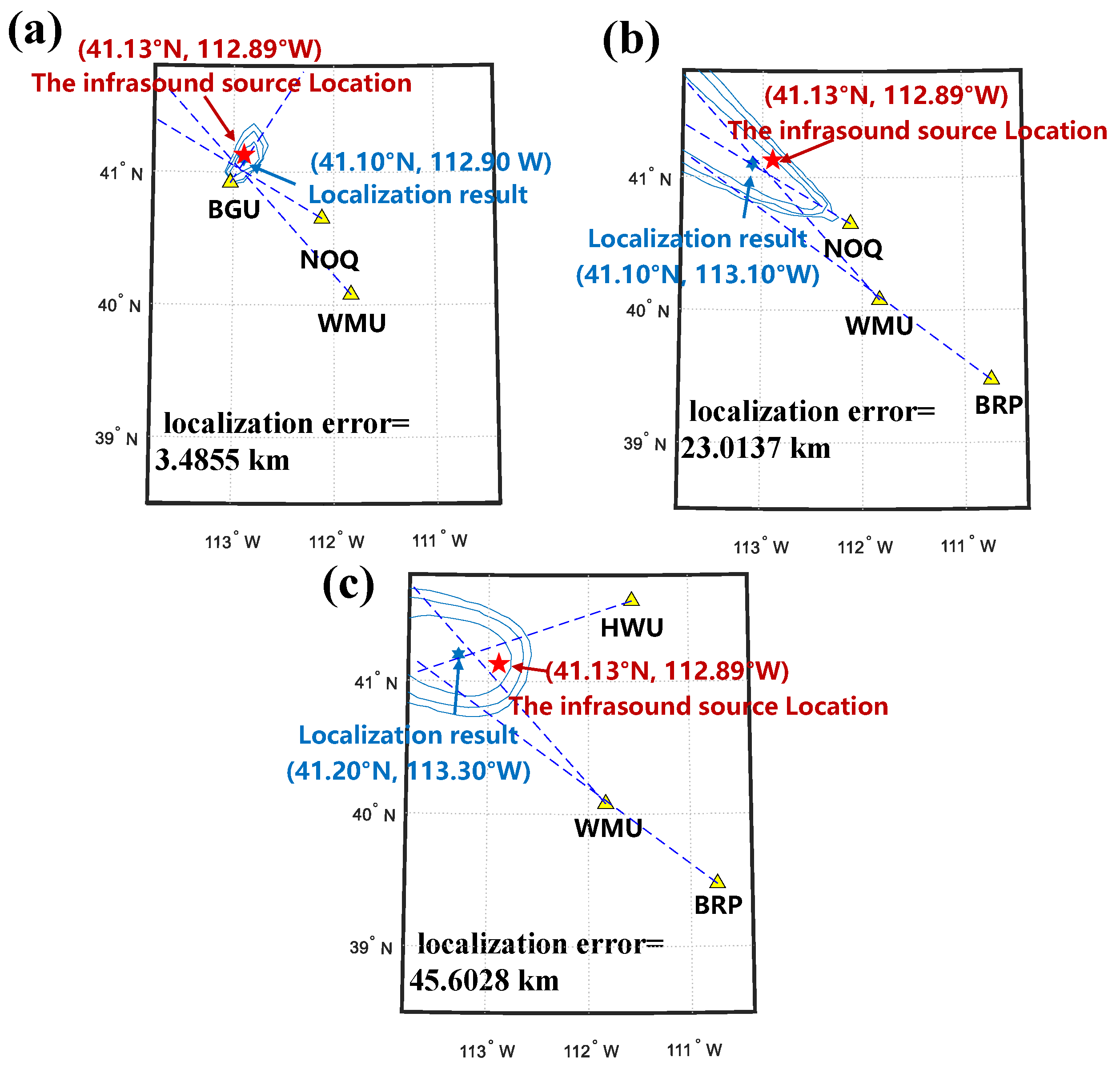
3.4. Bayesian Information Fusion to Obtain Localization Results

The arrival azimuth estimation results of the infrasound sources are affected by the uncertainty of the infrasound propagation and the infrasound measurement equipment. The uncertainty of the arrival azimuth estimation results is modeled by the Bayesian information fusion algorithm as the variance in a probabilistic model. The localization result of the infrasound source is the maximum value of the posterior probability density function. The credibility contour curve represents the possible area of the infrasound source. The localization results are shown in Figure 13.

Figure 13. The localization result of the infrasound source by fusing the SBL arrival azimuth estimations. (The three blue contour curves are credibility contour curves with Bayesian credibility values of 0.75, 0.90, and 0.95, respectively; the red pentagram indicates the location of the infrasound source; the blue hexagram indicates the distributed array localization results; and the enlarged scale is 1:10).

Figure 13. The localization result of the infrasound source by fusing the SBL arrival azimuth estimations. (The three blue contour curves are credibility contour curves with Bayesian credibility values of 0.75, 0.90, and 0.95, respectively; the red pentagram indicates the location of the infrasound source; the blue hexagram indicates the distributed array localization results; and the enlarged scale is 1:10).

In Figure 13, it can be seen that the infrasound source localization result and ground truth location are (41.10${}^{\circ }$N, 112.89${}^{\circ }$W) and (41.13${}^{\circ }$N, 112.89${}^{\circ }$W), respectively. The distance between the infrasound source and the localization result is 3.4855 km. Three of the curves shown in Figure 13 are credibility contour curves with Bayesian credibility values of 0.75, 0.90, and 0.95, respectively, which are the possible regions of the infrasound source. From the above localization results, it can be seen that accurate infrasound source localization results can be obtained by the proposed infrasound source algorithm for infrasound sources within 250 km distance from the infrasound station. The arrival azimuth estimation results from the FK analysis are used to obtain the infrasound source localization results using the Bayesian information fusion algorithm, which are shown in Figure 14.

Compared with Figure 13, the results of infrasound source localization are the same; both are 41.10${}^{\circ }$N, 112.90${}^{\circ }$W. From Table 4, it can be seen that the estimated errors of the arrival azimuths of the FK analysis are 2.02°, 4.62°, 1.18°, and 8.87° larger than those of the SBL for the four stations BGU, BRP, HWU, and WMU, respectively. The area of the credibility contour corresponding to the Bayesian credibility of 0.75 is 918.6532 km${}^2$ and 923.7934 km${}^2$ in Figure 13 and Figure 14, respectively. The area of the credibility contour corresponding to the Bayesian credibility of 0.75 obtained by the SBL is 5.1402 km${}^2$ smaller than that of the FK analysis, which means that the corresponding mode of the posterior probability density function is more concentrated (i.e., the posterior probability density function is visually sharper at the peak). The above results indicate that the proposed method is more reliable than the combination method of FK analysis and Bayesian information fusion.

4. Discussion

The performance of the proposed infrasound source localization algorithm is discussed in this section. The accuracy of the infrasound source localization is related to the number of stations involved in localization. The results of Bayesian information fusion localization for different number of stations are shown in Figure 15. As shown in Figure 15, the localization errors of two stations, three stations, and four stations are 78.3306 km, 13.0329 km, and 3.4855 km, respectively. It can be seen that the error of infrasound source localization is further reduced with the increase in the number of infrasound stations. The same conclusion can be obtained by performing Bayesian information fusion algorithm on the results of the FK analysis and beamforming.

It can be seen from Figure 16a that the four stations NOQ, BGU, WMU, and BRP are basically arranged in a straight line. By contrast, in Figure 16b, the azimuth of the HWU station with respect to the infrasound source is different from the azimuths of the BGU, WMU, and BRP stations. Therefore, the spatial distribution of the four stations with respect to the infrasound source in Figure 16b is more dispersed compared with that in Figure 16a. The localization error of the algorithm is also related to the arrangement of infrasound stations. The NOQ station is added in order to discuss whether the localization error of the proposed infrasound source localization algorithm is related to the arrangement of infrasound stations. The position of this infrasound station is (40.6526${}^{\circ }$N, 112.1180${}^{\circ }$W), and the arrival azimuths obtained by the SBL algorithm is 301.10°. When the station arrangement is more dispersed relative to the infrasound source, as shown in Figure 16a, the localization result is (41.10${}^{\circ }$N, 112.90${}^{\circ }$W). It can be seen that the arrangement of the stations has little influence on the localization error of the infrasound source localization algorithm proposed in this paper. The same conclusion can be obtained by performing the Bayesian information fusion algorithm on the results of the FK analysis and beamforming. In Figure 16, the area of the credibility contours corresponding to the Bayesian credibility value of 0.75 is 387.6142 km${}^2$ (Figure 16a) and 993.1705 km${}^2$ (Figure 16b), respectively. Therefore, the station arrangement has a certain influence on the credibility contour areas of the infrasound source localization result. The estimation error of the arrival azimuth of the HWU station is 0.99° larger than that of the NOQ station, but the localization error is the same for both arrangements. The impact on the final localization error can be reduced by the Bayesian information fusion algorithm when the estimation error of the arrival azimuth of a single station is 0.99° larger.

Next, we discuss the influence of the distance between the station and the infrasound source on the error of the localization results. In Figure 17, the sum of the distances from BGU, NOQ, and WMU stations to the infrasound source; the BRP, NOQ, and WMU stations to the infrasound source; and the BRP, HWU, and WMU stations to the infrasound source are 295.1944 km, 569.0806 km, and 624.5797 km, respectively. The errors of the infrasound source localization for these three cases are 3.4855 km, 23.0137 km, and 45.6028 km, respectively. As can be seen from Figure 17, the localization error of the algorithm increases as the stations are arranged farther away relative to the infrasound source. Therefore, it is necessary to select the stations that are arranged closer to the infrasound source for analysis to obtain accurate infrasound source localization results. The same conclusion can be obtained by performing the Bayesian information fusion algorithm on the results of the FK analysis and beamforming.

5. Conclusions

The precise localization of infrasound sources is a problem of considerable interest. The infrasound source localization can be affected by the atmospheric environment and infrasound measurement equipments, resulting in poor accuracy of infrasound source localization. In this paper, the SBL algorithm is applied to infrasound source arrival azimuth estimation for the first time. The uncertainties in the atmospheric environment and measurement equipments can be modeled as the variance in the Bayesian information fusion algorithm. The maximum value of posterior probability is used as the infrasound source localization result. Infrasound source credibility contours with Bayesian credibility values of 0.75, 0.90 and 0.95, respectively, are obtainable by the Bayesian information fusion algorithm. Subsequently, rocket motor explosion infrasound data obtained in UTTR were used to verify feasibility of the algorithm. The infrasound signals recorded at the four infrasound stations are processed by the SBL algorithm and the Bayesian information fusion algorithm. The analysis of the measured data shows that the arrival azimuth estimation angle error of the SBL algorithm is within 2°. The arrival azimuth estimation accuracy is significantly improved, compared with the FK analysis and beamforming. Finally, the Bayesian information fusion algorithm is used to fuse the information of multiple stations to obtain the localization results of infrasound sources. The analysis of the measured data shows that for the infrasound source within 250 km from the infrasound station, the error of the positioned infrasound source distance is within 3.5 km.

In summary, (i) the SBL algorithm is applied to infrasound source localization in this paper, which significantly reduces the estimation error of the arrival azimuth; (ii) the Bayesian information fusion algorithm is used to incorporate the uncertainty brought by the infrasound propagation environment and the measurement equipment into the infrasound source localization, making the localization results more robust.

References

1. Le Pichon, A.; Blanc, E.; Hauchecorne, A. Infrasound Monitoring for Atmospheric Studies; Springer Science & Business Media: Berlin/Heidelberg, Germany, 2010. [Google Scholar]
2. Freret-Lorgeril, V.; Bonadonna, C.; Corradini, S.; Donnadieu, F.; Guerrieri, L.; Lacanna, G.; Marzano, F.S.; Mereu, L.; Merucci, L.; Ripepe, M.; et al. Examples of Multi-Sensor Determination of Eruptive Source Parameters of Explosive Events at Mount Etna. Remote Sens. 2021, 13, 2097. [Google Scholar] [CrossRef]
3. Cigna, F.; Tapete, D.; Lu, Z. Remote Sensing of Volcanic Processes and Risk. Remote Sens. 2020, 12, 2567. [Google Scholar] [CrossRef]
4. Batubara, M.; Yamamoto, M.-y. Infrasound Observations of Atmospheric Disturbances Due to a Sequence of Explosive Eruptions at Mt. Shinmoedake in Japan on March 2018. Remote Sens. 2020, 12, 728. [Google Scholar] [CrossRef] [Green Version]
5. De Angelis, S.; Diaz-Moreno, A.; Zuccarello, L. Recent Developments and Applications of Acoustic Infrasound to Monitor Volcanic Emissions. Remote Sens. 2019, 11, 1302. [Google Scholar] [CrossRef] [Green Version]
6. Mutschlecner, J.P.; Whitaker, R.W. Infrasound from earthquakes. J. Geophys. Res. Atmos. 2005, 110. [Google Scholar] [CrossRef] [Green Version]
7. Garces, M.; Pichon, A.L. Infrasound from Earthquakes, Tsunamis and Volcanoes. In Encyclopedia of Complexity and Systems Science; Springer: New York, NY, USA, 2011; pp. 663–679. [Google Scholar] [CrossRef]
8. Laiolo, M.; Ripepe, M.; Cigolini, C.; Coppola, D.; Della Schiava, M.; Genco, R.; Innocenti, L.; Lacanna, G.; Marchetti, E.; Massimetti, F.; et al. Space- and Ground-Based Geophysical Data Tracking of Magma Migration in Shallow Feeding System of Mount Etna Volcano. Remote Sens. 2019, 11, 1182. [Google Scholar] [CrossRef] [Green Version]
9. Rost, S.; Thomas, C. Array Seismology: Methods and Applications. Rev. Geophys. 2002, 40, 2-1–2-27. [Google Scholar] [CrossRef] [Green Version]
10. Tipping, M.E. Sparse Bayesian learning and the relevance vector machine. J. Mach. Learn. Res. 2001, 1, 211–244. [Google Scholar]
11. Wipf, D.; Rao, B. Sparse Bayesian learning for basis selection. IEEE Trans. Signal Process. 2004, 52, 2153–2164. [Google Scholar] [CrossRef]
12. Zhang, Z.; Rao, B.D. Sparse Signal Recovery With Temporally Correlated Source Vectors Using Sparse Bayesian Learning. IEEE J. Sel. Top. Signal Process. 2011, 5, 912–926. [Google Scholar] [CrossRef] [Green Version]
13. Gerstoft, P.; Mecklenbräuker, C.F.; Xenaki, A.; Nannuru, S. Multisnapshot Sparse Bayesian Learning for DOA. IEEE Signal Process. Lett. 2016, 23, 1469–1473. [Google Scholar] [CrossRef] [Green Version]
14. Gemba, K.L.; Nannuru, S.; Gerstoft, P. Robust Ocean Acoustic Localization With Sparse Bayesian Learning. IEEE J. Sel. Top. Signal Process. 2019, 13, 49–60. [Google Scholar] [CrossRef]
15. Nannuru, S.; Gemba, K.L.; Gerstoft, P.; Hodgkiss, W.S.; Mecklenbräuker, C.F. Sparse Bayesian learning with multiple dictionaries. Signal Process. 2019, 159, 159–170. [Google Scholar] [CrossRef] [Green Version]
16. Liu, Z.M.; Huang, Z.T.; Zhou, Y.Y. An Efficient Maximum Likelihood Method for Direction-of-Arrival Estimation via Sparse Bayesian Learning. IEEE Trans. Wirel. Commun. 2012, 11, 1–11. [Google Scholar] [CrossRef]
17. Chen, S.S.; Donoho, D.L.; Saunders, M.A. Atomic Decomposition by Basis Pursuit. SIAM Rev. 2001, 43, 129–159. [Google Scholar] [CrossRef] [Green Version]
18. Garcés, M.A.; Hansen, R.A.; Lindquist, K.G. Traveltimes for infrasonic waves propagating in a stratified atmosphere. Geophys. J. Int. 1998, 135, 255–263. [Google Scholar] [CrossRef] [Green Version]
19. Modrak, R.T.; Arrowsmith, S.J.; Anderson, D.N. A Bayesian framework for infrasound location. Geophys. J. Int. 2010, 181, 399–405. [Google Scholar] [CrossRef] [Green Version]
20. Drob, D.P.; Garcés, M.; Hedlin, M.; Brachet, N. The temporal morphology of infrasound propagation. Pure Appl. Geophys. 2010, 167, 437–453. [Google Scholar] [CrossRef]
21. Wipf, D.P.; Rao, B.D. An Empirical Bayesian Strategy for Solving the Simultaneous Sparse Approximation Problem. IEEE Trans. Signal Process. 2007, 55, 3704–3716. [Google Scholar] [CrossRef]
22. Bohme, J. Source-parameter estimation by approximate maximum likelihood and nonlinear regression. IEEE J. Ocean. Eng. 1985, 10, 206–212. [Google Scholar] [CrossRef]
23. Ji, S.; Xue, Y.; Carin, L. Bayesian Compressive Sensing. IEEE Trans. Signal Process. 2008, 56, 2346–2356. [Google Scholar] [CrossRef]
24. Blom, P.S.; Marcillo, O.; Arrowsmith, S.J. Improved Bayesian Infrasonic Source Localization for regional infrasound. Geophys. J. Int. 2015, 203, 1682–1693. [Google Scholar] [CrossRef] [Green Version]
25. Stump, B.; Burlacu, R.; Hayward, C.; Pankow, K.; Nava, S.; Bonner, J.; Hock, S.; Whiteman, D.; Fisher, A.; Kim, T.S. Seismic and Infrasound Energy Generation and Propagation at Local and Regional Distances Phase 1-Divine Strake Experiment; Southern Methodist University: Dallas, TX, USA, 2008. [Google Scholar]
26. Arrowsmith, S.J.; Whitaker, R.; Taylor, S.R.; Burlacu, R.; Stump, B.; Hedlin, M.; Randall, G.; Hayward, C.; ReVelle, D. Regional monitoring of infrasound events using multiple arrays: Application to Utah and Washington State. Geophys. J. Int. 2008, 175, 291–300. [Google Scholar] [CrossRef] [Green Version]
27. Stump, B.W.; Zhou, R.M.; Kim, T.S.; Chen, Y.T.; Yang, Z.X.; Herrmann, R.B.; Burlacu, R.; Hayward, C.; Pankow, K. Shear Velocity Structure in NE China and Characterization of Infrasound Wave Propagation in the 1–210 km Range; Southern Methodist University: Dallas, TX, USA, 2008. [Google Scholar]
28. Capon, J.; Bolt, B. Signal processing and frequency-wavenumber spectrum analysis for a large aperture seismic array. In Methods in Computational Physics; Elsevier: Amsterdam, The Netherlands, 1973; Volume 13, pp. 1–59. [Google Scholar]
29. Aki, K.; Richards, P.G. Quantative seismology: Theory and methods. Earth Sci. Rev. 1981, 17, 296–297. [Google Scholar]
30. Shani-Kadmiel, S.; Averbuch, G.; Smets, P.; Assink, J.; Evers, L. The 2010 Haiti earthquake revisited: An acoustic intensity map from remote atmospheric infrasound observations. Earth Planet. Sci. Lett. 2021, 560, 116795. [Google Scholar] [CrossRef]
Figure 1. Propagation trajectory of the tau-p model in a phase loop, the azimuth angle θ , the angle of elevation ϕ , the altitude of infrasound propagation z, the infrasound propagation distance R of a phase loop in Equation (2), the maximum altitude z m a x that a phase loop can propagate, and the transverse offset Q of infrasound propagation in Equation (4) (the red arrow and red dot indicate the direction of infrasound propagation at the starting point and the location of the maximum elevation of infrasound propagation, respectively).
Remotesensing 14 03181 g001
Figure 2. Schematic diagram of infrasound three-dimensional propagation under the assumption of plane waves. (The z-axis is the infrasound propagation height, which corresponds to the z-axis in Figure 1. u is the wave number vector; c is the sound velocity; r is the position vector; P is the acoustic signal when the initial time is t; and α , β are the angle values).
Remotesensing 14 03181 g002
Figure 3. The structure diagram of Bayesian hierarchical model (blue rectangules denote the known parameters; red circles denote the unknown parameters). The initialized infrasound source power parameters γ 0 are used to update the parameters γ in the Equation (28), and the initialized infrasound source noise variance parameters σ 0 are used to update the parameters σ in the Equation (33).
Remotesensing 14 03181 g003
Figure 4. The schematic diagram for Bayesian information fusion algorithm. (a) SBL:SBL-based infrasound signal processing of stations to obtain the azimuth of stations (azimuth = θ 1 , θ 2 , , θ N ); (b) Bayesian information fusion:information fusion of station-acquired azimuths using Bayesian information fusion to obtain localization results (red pentagrams indicate localized infrasound source locations, yellow triangles indicate infrasound stations, and the three blue contour lines are credibility curves with different Bayesian credibility values).
Remotesensing 14 03181 g004
Figure 5. The technical flowchart of the infrasound source localization algorithm proposed in this paper. The first step is to estimate the arrival azimuth by the SBL algorithm by updating the hyperparameter gamma using Equation (28). The estimated value of the arrival azimuth is the angle corresponding to the γ m a x . The second step is the Bayesian information fusion for infrasound source localization. The posterior PDF maximum value is the infrasound source location m = ( x , y ) .
Remotesensing 14 03181 g005
Figure 6. The array structures of BGU, BRP, HWU, and WMU are shown in (ad), respectively.
Remotesensing 14 03181 g006
Figure 7. Time domain signal after 1-5 Hz filtering for four stations: (a) the total signal duration of the BGU station is 20 s; (b) the total signal duration of the BRP station is 30 s; (c) the total signal duration of the HWU station is 100 s; and (d) the total signal duration of the WMU station is 15 s.
Remotesensing 14 03181 g007
Figure 8. The process of converting infrasound signals from the time domain to the frequency domain using the snapshot method. The variable d m is the observed position of the m-th sensor, and the variable L is the total number of snapshots.
Remotesensing 14 03181 g008
Figure 9. The results of the SBL algorithm for four infrasound stations (the angular resolution Δ θ is 0.1°): (a) the SBL algorithm arrival azimuth estimation result for the BGU station is 27.2°; (b) the SBL algorithm arrival azimuth estimation result for the BRP station is 44.5°; (c) the SBL algorithm arrival azimuth estimation result for the HWU station is −38.4°; and (d) the SBL algorithm arrival azimuth estimation result for the WMU station is 27.9°.
Remotesensing 14 03181 g009
Figure 10. The azimuths obtained from the BGU station, BRP station, HWU station, and WMU station are (a) 32.91°, (b) 307.35°, (c) 252. 07°, and (d) 314.35°, respectively (the array tilt angle is defined as the acute angle between a linear array of two array sensors and the latitude line in the geographic coordinate system).
Remotesensing 14 03181 g010
Figure 11. The azimuths from the FK analysis of the BGU, BRP, HWU, and WMU stations are (a) 29.05°, (b) 312.13°, (c) 247.83°, and (d) 323.53°, respectively.
Remotesensing 14 03181 g011
Figure 12. The results from the beamforming of the BGU, BRP, HWU, and WMU stations are (a) 23.8°, (b) 41.1°, (c) −41.3°, and (d) 26.9°, respectively.
Remotesensing 14 03181 g012
Figure 14. The localization result of the infrasound source by fusing the FK arrival azimuth estimations. (The three blue contour curves are credibility contour curves with Bayesian credibility values of 0.75, 0.90, and 0.95, respectively; the red pentagram indicates the location of the infrasound source; and the blue hexagram indicates the distributed array localization results).
Remotesensing 14 03181 g014
Figure 15. Localization errors for different numbers of stations (arrival azimuth estimation results from the SBL algorithm); (a) 78.3306 km for two stations (HWU and BRP); (b) 13.0329 km for three stations (BGU, HWU, and BRP); and (c) 3.4855 km for four stations (BGU, HWU, BRP, and WMU).
Remotesensing 14 03181 g015
Figure 16. The influence of the spatial distribution of infrasound stations on the localization results (arrival azimuth estimation results from the SBL algorithm); (a) BGU, NOQ, WMU, and BRP; (b) BGU, HWU, WMU, and BRP.
Remotesensing 14 03181 g016
Figure 17. The influence of the distance between the station and the infrasound source on the error of localization result (arrival azimuth estimation results from the SBL algorithm); (a) the sum of the distances from the BGU, NOQ, and WMU stations to the infrasound source is 295.1944 km; (b) the sum of the distances from the BRP, NOQ, and WMU stations to the infrasound source is 569.0806 km; and (c) the sum of the distances from BRP, HWU, and WMU stations to the infrasound source is 624.5797 km.
Remotesensing 14 03181 g017