Article

A Statistical Approach to Using Remote Sensing Data to Discern Streamflow Variable Influence in the Snow Melt Dominated Upper Rio Grande Basin

1
New Mexico Water Resources Research Institute, New Mexico State University, Las Cruces, NM 88001, USA
2
USDA Southwest Climate Hub, Jornada Experimental Range, Las Cruces, NM 88003, USA
*
Author to whom correspondence should be addressed.
Remote Sens. 2022, 14(23), 6076; https://doi.org/10.3390/rs14236076
Submission received: 23 September 2022 / Revised: 26 November 2022 / Accepted: 28 November 2022 / Published: 30 November 2022
(This article belongs to the Special Issue Applications of Remotely Sensed Data in Hydrology and Climatology)

Abstract

:
Since the middle of the 20th century, the peak snowpack in the Upper Rio Grande (URG) basin of United States has been decreasing. Warming influences snowpack characteristics such as snow cover, snow depth, and Snow Water Equivalent (SWE), which can affect runoff quantity and timing in snowmelt runoff-dominated river systems of the URG basin. The purpose of this research is to investigate which variables are most important in predicting naturalized streamflow and to explore variables’ relative importance for streamflow dynamics. We use long term remote sensing data for hydrologic analysis and deploy R algorithm for data processing and synthesizing. The data is analyzed on a monthly and baseflow/runoff basis for nineteen sub-watersheds in the URG. Variable importance and influence on naturalized streamflow is identified using linear standard regression with multi-model inference based on the second-order Akaike information criterion (AICc) coupled with the intercept only model. Five predictor variables: temperature, precipitation, soil moisture, sublimation, and SWE are identified in order of relative importance for streamflow prediction. The most influential variables for streamflow prediction vary temporally between baseflow and runoff conditions and spatially by watershed and mountain range. Despite the importance of temperature on streamflow, it is not consistently the most important factor in streamflow prediction across time and space. The dominance of precipitation over streamflow is more obvious during baseflow. The impact of precipitation, SWE, sublimation, and minimum temperature on streamflow is evident during the runoff season, but the results vary for different sub-watersheds. The association between sublimation and streamflow is positive in the runoff season, which may relate to temperature and requires further research. This research sheds light on the primary drivers and their spatial and temporal variability on streamflow generation. This work is critical for predicting how warming temperatures will impact water supplies serving society and ecosystems in a changing climate.

1. Introduction

The Rio Grande is deemed one of the most threatened rivers of the Western United States [1] and observed snowpack in the Upper Rio Grande (URG) basin is not producing the expected runoff per unit of snowpack volume [2]. Various sources have already cited drying of the URG [3,4]. The Rio Grande River is the main source of irrigation and municipal water within the URG basin [5]. It supplies drinking water to more than 6 million people and irrigation water to 2 million acres of land [6].
The purpose of this study is to examine which mechanisms are most influential on streamflow dynamics in sub-watersheds of the URG basin. Increasing temperatures and decreasing snowpack from heightened snow albedo are deemed as the main drivers reducing streamflow. Regional climate change in the Southwestern US will likely continue [7] to affect streamflow dynamics, highlighting the need to better understand streamflow variables’ influences in the region.
Understanding which variables control streamflow and when they are important is essential for accurately predicting streamflow. Rather than prediction, this study determines the relative importance of variables known to influence naturalized streamflow dynamics. We expect their relative importance to vary temporally and spatially between watersheds.
This study explores the following research questions: (1) which are the most influential variables for streamflow dynamics? (2) What is the rank of each candidate variable as relative importance? Finally, (3) how does this relative importance change over the year for different watersheds? Using multiple linear regression models, we employed multimodal inference (MMI) based on the second-order Akaike Information Criterion (AICc) and computed model-averaged estimates to answer these questions.
Previous studies explore various established approaches to evaluate variable influence in estimating runoff [2,5,8,9,10,11,12,13,14,15,16,17,18]; however, very few of these studies have addressed the dynamic nature of the influences from a statistical approach. Consequently, there is relatively little information available about the variability of variable influence on streamflow at a catchment scale, but it is also critical to understand the dynamics of parameters’ influence on runoff when focusing on improving prediction accuracy. Many studies overlook this part while selecting models or assessing performances. We found no study exclusively dedicated to exploring catchment-based variable importance. Thus, the novelty of this article is that it first advanced this investigation as an inquiry into variable importance, ranked them, and analyzed the dynamics of influences on streamflow in the study area. Exploring the region-specific watershed parameters, the article produced a large amount of hydrologic information that can support the forecasting effort by filling out the information gap in the literature regarding variable importance.

1.1. Estimating Streamflow: The Response Variable

The Upper Rio Grande (URG) basin has been experiencing downward trends in peak snowpack from 1951 to 2015, but a consequential long-term decline was not observed in the streamflow record [2]. Streamflow has slightly declined in the snowmelt runoff season from April–July, but small increases in precipitation offset this trend in streamflow [2]. However, Lehner at al. (2017) showed a declining trend in the runoff ratio from the 1980s to recent date [8]. They also explained that very low runoff ratios are more likely to be associated with above-normal temperatures [8]. This is an indication of further runoff declination under a continuously warming climate.
Different modeling groups use different variables and techniques when estimating runoff. NRCS uses statistical models that are based on multiple linear regressions, fitting a mathematical relationship between predictor variables and target variables, expressed through equations [9]. NRCS uses several predictor variables for the regression model used to predict seasonal streamflow volume [9,10]. Generally, these predictor variables are Snow Water Equivalent (SWE), precipitation, and antecedent streamflow [5,10]. Other variables, such as temperature, groundwater levels, and soil water content, are also considered [5]. Permafrost conditions and snow cover distributions are critical for the ecohydrological process of watershed, which is substantially connected to the water supply system of the region. Studying several variables such as soil temperature, active-layer thickness (alt), vegetation conditions, etc., at a landscape scale, Zhang et al. found that the factors influencing permafrost thaw spatially and seasonally vary. These parameters are sensitive to the warming climate and have long-term hydrological and ecological implications [11]. Seasonal and temporal variation, along with the degrading pattern of permafrost, can influence runoff quantity and timing by influencing water release that contributes to the runoff pattern of the region.
However, persistent prediction errors were observed for spring and summer runoff in several watersheds in the Southwestern US [5]. These errors are mostly driven by decadal precipitation trends and the effect of increasing temperatures [12]. Inclusion of seasonal temperature forecasts from the Global Circulation Model (GCM) can sufficiently reduce forecast errors in the snowmelt-driven streamflow [12]. Likewise, the UA SWE tool (University of Arizona Snow Water Equivalent tool) provides better accuracy to estimate SWE because it considers projected temperature and precipitation along with the station-based snow depth and SWE observed in various sites [13].
The active radar-based sensors can play a significant role in monitoring variables’ variability in influencing the freeze–thaw of snow cover. Radar remote sensing has powerful applications, such as synthetic aperture radar (SAR), that are adequately able to capture and monitor the spatial and temporal heterogeneity of the thawing pattern of permafrost [14]. Touzi’s (2006) new scattering vector model allows a polarization basis invariant for the representation of coherent target scattering, which is promising for wetland assessment and classification [15]. Microwave radar is considered another reliable tool for monitoring snow cover variability because it has an ability to address the dielectric properties of snow [16].
The advent of novel techniques in the domain of optical remote sensing (ORS) has enriched its ability to map snow cover and permafrost conditions; ORS is now capable of addressing the spatial and temporal variability of snow factors [14]. Theia Snow collection routinely generates some high-resolution maps where snow cover is accurately detected through Sentinel-2 and Landsat-8 observations. Theia Snow products have been successfully applied for the evaluation of MODIS snow products; Gascoin (2019) discussed its potential applications in permafrost distribution modeling, hydrologic modeling, and spatial modeling of ecosystems in mountain regions [17]. However, as an optical-based observation system, the Theia Snow collection can’t always adequately define high spatial variability of snowpack properties, because optical sensors (e.g., MODIS) can’t capture snow cover below the canopy. Kostsfinov et al., (2019) developed a lidar-based method to detect snow cover under the canopy by investigating fractional snow cover areas [18].

1.2. The Predictor Variables

This study investigates various watershed factors affecting streamflow dynamics during runoff in a warming climate. These eight non-mutually exclusive variables include warming temperature, snow cover, snow depth, snow water equivalent, snow albedo, precipitation, soil moisture, and sublimation.
Decreases in snowpack in the Southwestern United States (US) are coupled with significant upward trends in temperature. The entire Southwest has been experiencing higher than average temperatures (i.e., 2 °F warmer than the long-term average in some areas) [19]. Warming can influence snowpack characteristics such as snow cover, snow depth, and Snow Water Equivalent (SWE), which can consequently impact runoff quantity and timing in snowmelt runoff-dominated river systems of the URG basin [20]. Snow cover is one of the key drivers that influences water supplies in the snowmelt-dominated river system, and mapping snow cover is thereby critical for understanding the snowmelt runoff hydrology of the catchment [18]. Snow cover is affected by climate change; however, it also can affect the climate. Unlike other darker surfaces, the whiteness of snow reflects solar radiation back to the space, absorbing a small portion (10–20%) of energy [21]. That means, more snow cover reflects more energy back to the space, cooling the Earth’s surface, while less snow cover reflects less energy and heat up to the surface, absorbing more energy. Thus, snow cover influences the heating and cooling system of the Earth’s surface; spatial distribution of snow cover is quantified by snow depth [22].
SWE is considered one of the critical factors used to enhance the prediction accuracy of snowmelt runoff and streamflow forecasting [23,24] because the spatial variability of SWE can largely influence the timing and amount of snowmelt runoff delivery to a watershed [25]. Taking care of the variability of SWE in a hydrologic model can improve accuracy in simulating snowmelt runoff dynamics.
Increasing desert dust changes snow albedo by allowing more absorption of solar radiation, which accelerates snowmelt rates and eventually shortens the duration of snow cover [26,27]. Changes in snow albedo and increasing temperature can facilitate more absorption of latent heat to the snowpack that triggers the rate of sublimation [28], which eventually causes snowpack reduction [29]. Earlier runoff occurs as a consequence, resulting in reduced water supplies post-runoff [26,27,30].
Reduced snowfall and simultaneously increased rainfall are a plausible cause of snowpack reduction, later affecting estimated runoff volume [2]. Soil moisture is also considered an important factor for streamflow dynamics, contributing moisture from snowmelt runoff and precipitation [31]. Lapp et al. (2005) anticipated that increased sublimation due to the upward trend in temperature and lower snow albedo from increased dust are the contributing factors to snowpack reduction, affecting runoff volume in the URG basin [28,29].

2. Materials and Methods
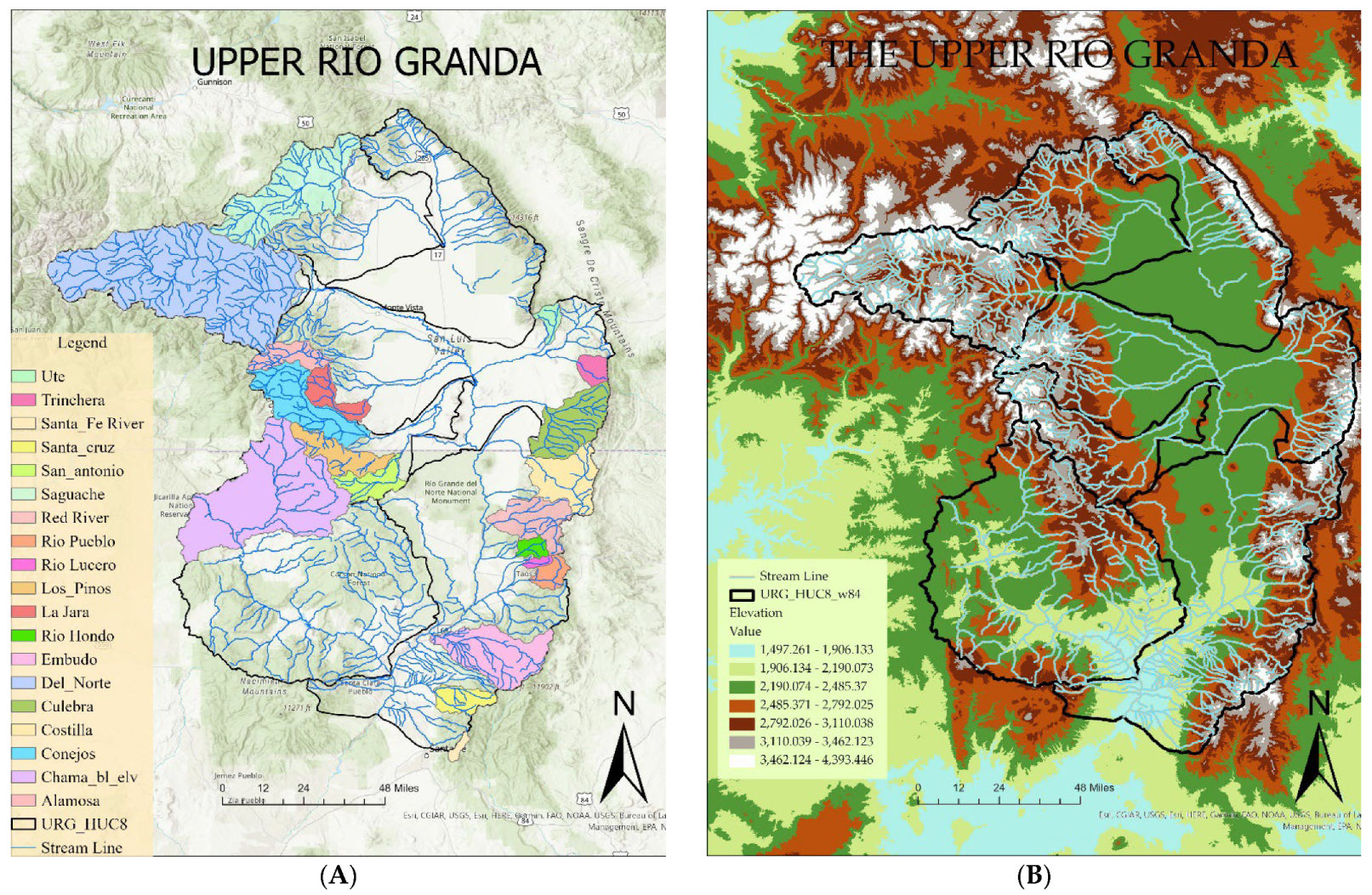
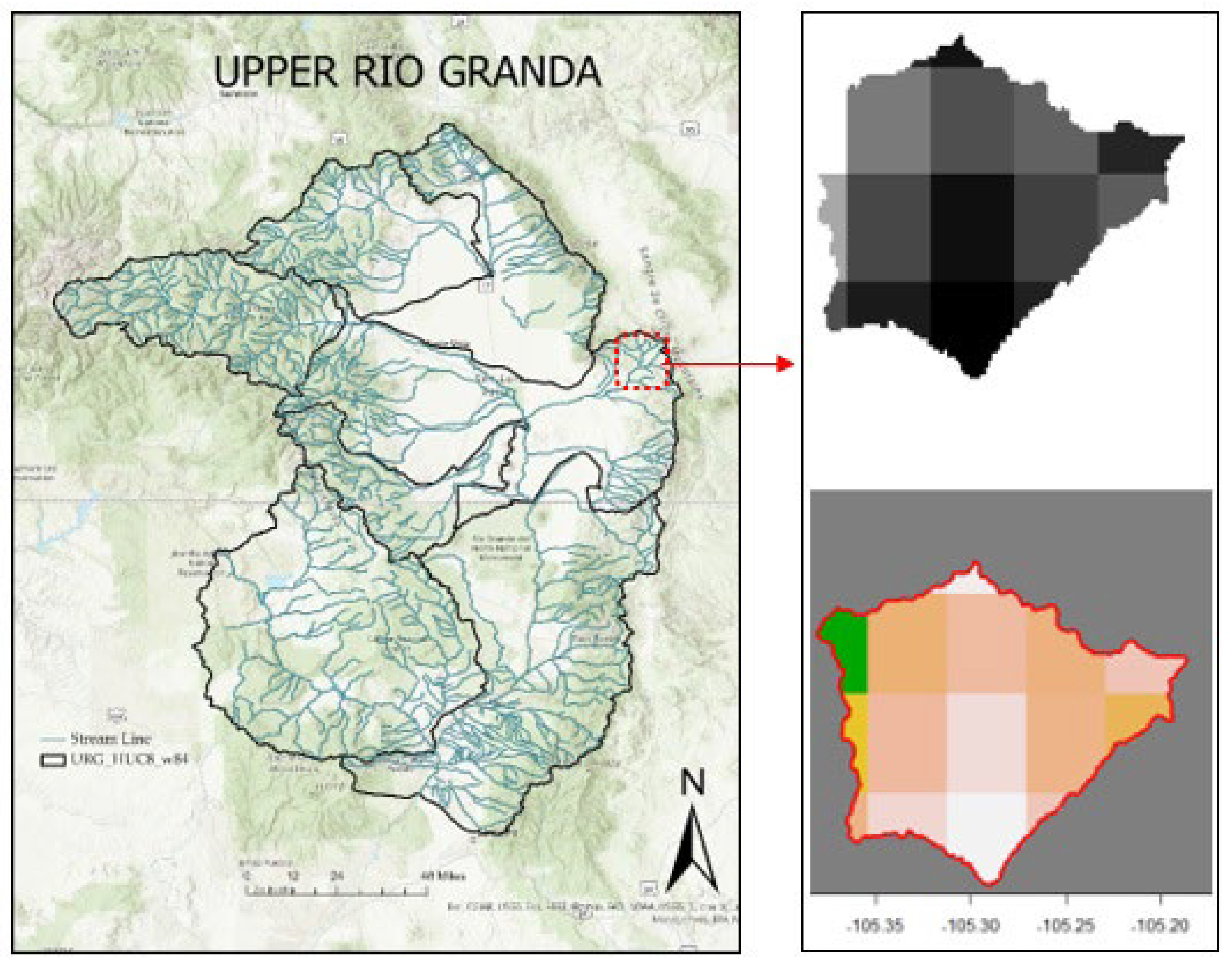
2.1. Study Area

The Upper Rio Grande basin (Figure 1A) is located on the border of Southern Colorado and Northern New Mexico, USA. Nineteen sub-watersheds are distributed among 3 mountain groups: The Southern San Juan, The Central Sangre De Cristo, and The Southern Sangre De Cristo. In the following Figure 1, the ESRI’s ‘USA Detail Streams’ layer [32] was used to show the detailed rivers and streams. The Rio Grande flows from its source, the San Juan Mountains, and runs towards lower elevation to the southeast (Figure 1B). Many watersheds of the basin are intermittent by nature, and the flow varies accordingly (Appendix B). Del Norte, Rio Chama, and Conejos watersheds have the higher streamflow volume recorded through the year; all these three watersheds are located in the Southern San Juan mountain range.
The nineteen sub-watersheds are delineated using existing USGS gauging stations and digital Elevation Models (DEM) (Table 1). To comprehensively analyze watershed variables, all the components’ underlying data must be acquired. We could acquire complete information from the sources cited (Table 2) to adequately analyze the selected 19 watersheds. Elevation data are extracted using ArcGIS 10.0 [33]; DEMs are downloaded from the National Elevation Dataset [34], produced and distributed by the USGS [35].

2.2. Data Description

Eight predictor variables are considered in this study: temperature, SWE, snow cover, snow depth, snow albedo, precipitation, soil moisture, and sublimation. We collected monthly time step predictor and response variable data from various sources (Table 2) for a 39-year period (August 1980 to July 2019) for 19 sub-watersheds of the URG basin.

Data Processing

This study deploys R studio [44] for data processing and statistical analysis. We chose to use R to clip raster data for its ability to incorporate watershed border cells, a feature which ArcMap lacks (Figure 2). For each sub-watershed, we disaggregated original monthly raster cells to 30 × 30 m cells to be clipped to sub-watershed boundaries. Monthly responses for the sub-watersheds are calculated as the average of the disaggregated pixels; centroids were within the watershed boundary.
We used NRCS-adjusted naturalized streamflow data (monthly volume) in the analyses (Appendix A); the naturalized streamflow occasionally has some negative flow values. The negative values are a result of the naturalization process that NRCS uses for their streamflow datasets. The basins have significant regulation though reservoir storage or direct diversion, and NRCS adjusted the volume observed at the stream gage to account for this regulation when the data are available. Unfortunately, not all extractions accounted for lack of precision. This can lead to negative values in some cases during very dry years or low flow months. The streamflow values should be either zero or positive and these negative values are the error of the system. This error especially occurs in some cases during a very dry year period or low flow period. Moreover, most of our nineteen watersheds are intermittent by nature (Appendix A) [45,46]. Therefore, we treated these negative streamflow values as zero in our analyses.

2.3. AICcmodavg’ Package and Second-Order Akaike Information Criterion (AICc)

The ‘AICcmodavg’ package uses applications for model selection and multimodal inference (classic model averaging) for various types of models based on different information criteria i.e., Akaike information criterion (AIC), second-order AIC (AICc), QAIC, QAICc, and BIC (Bayesian). It has certain types of goodness-of-fit statistics; the package also includes features to compute relative variable importance, evidence ratios, and confidence sets for the top model [47,48].
AICc is particularly suitable for assessing relative variable importance in candidate models [47,48]. AICc is a modified version of the more well-known AIC that is adjusted for small sample size (>~30) [49]. Unlike Bayesian Information Criteria (BIC), AICc does not assume that the “true” model exists in the candidate model set [50]. Following Cade (2015), this method standardizes the predictor variables and streamflow values prior to performing regressions [51]. This changes the interpretation of the regression coefficients; for example, a predictor variable with a standardized regression coefficient of 0.5 implies that an increase in the variable by one standard deviation would result in an increase in streamflow by 0.5 standard deviations. This enables AICc-weighted model averaging, but interpretations must be informed by acknowledging the distributional differences over time. For example, in the Rio Chama sub-watershed, one standard deviation of streamflow in January is 1952-acre feet and increases to 59,117-acre feet in May, while the corresponding standard deviations of minimum temperature are 2.02 and 0.976 degrees Celsius, respectively.

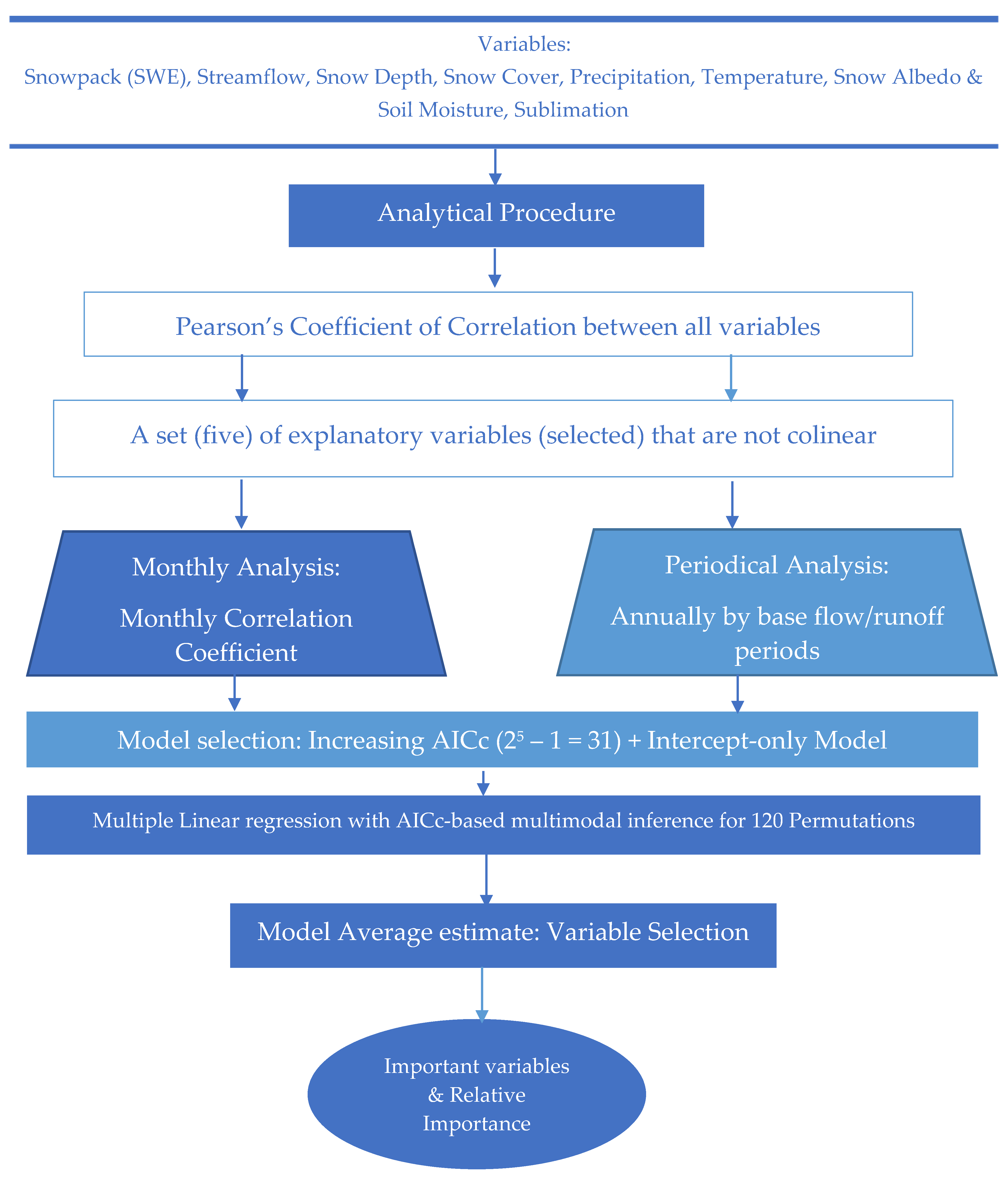
2.4. Analytical Procedure

Data for each variable are proportioned into the months of the year for each year on record, so that each variable is categorized by a given month from 1980 to 2020. We first determined the collinearity of the eight collected variables through Pearson’s correlation coefficient to retain variables that are not collinear. Five predictor variables are retained for monthly and annual response analyses. These predictor variables are sublimation, SWE, soil moisture, minimum temperature, and precipitation.
Next, Pearson’s correlation coefficients are calculated between streamflow and the retained variables for each month of the year to observe relationship changes over the year. For the annual responses, we use the operational water year which begins in August and ends in July of the next year. Linear regression analyses are conducted at monthly and annual base flow and runoff period temporal scales for each sub-watershed. Base flow is from August to February and runoff is from March to July.
Rather than developing a different conceptual model for each sub-watershed and temporal scale, we construct a candidate model set of all possible combinations of the five variables, yielding 25 − 1 = 31 possible models for each sub-watershed. We then examined each temporal scale combination for each sub-watershed using AICc-based multimodal inferences to determine variable importance. In addition to the 31 possible models, we also include an intercept-only model to account for model uncertainty. After fitting all models in each model set, we rank them by order of increasing AICc. In cases where the intercept-only model is within two AICc units of the best fitting model we conclude that none of the predictor models naturalized streamflow effectively. When the intercept-only model is not within two AICc units of the best-fitting model, we use the ‘AICcmodavg’ package to compute AICc-weighted model-averaged estimates of each predictor [36,37].
AICc cannot accurately assess model uncertainty when there is multicollinearity among the predictor variables [51]. To account for this, we also assess bivariate Pearson correlations between variables in each model set and remove one of the variables in cases where the correlation was greater than ±0.4, resulting in a smaller number of candidate variables and therefore a smaller candidate model set. It is necessary to implement a ranking method to decide which variable to remove in each case where correlation exceeded the ±0.4 threshold. Since we observed that different rankings changed the results (an interesting finding on its own), we conclude that limiting the process to a single ranked set of variables would reveal only a part of the entire picture. Therefore, we repeated the process for the 5!/(5 − 5)! = 120 permutations of different possible rankings of the five variables, calculating the AICc-weighted model-averaged estimates for each of the 120 possible orders to accommodate all the possible rankings. We then averaged over the 120 permutations to produce an overall model-averaged estimate. This analytical strategy has never been documented as an approach to explore variable influence in watersheds. Following is the procedural flowchart (Figure 3) for the study.

3. Results

Of the eight initial variables, five noncollinear variables were initially selected, and then the study investigated how these variables affect normalized streamflow in 19 sub-watersheds on a monthly and seasonal basis. Our results indicate that several variables are significantly associated with naturalized streamflow in the Upper Rio Grande basin; however, the association varies both temporally and spatially. Temperature and precipitation are the most influential factors affecting naturalized streamflow in the URG sub-watersheds. The combination of variables impacting streamflow is not consistent, varying over time and by sub-watershed.

3.1. Predictor and Response Variable Colinearity

The study calculated Pearson’s coefficients of correlation (r) among all the variables for each sub-watershed (Correlation Table: Supplementary File). Albedo and snow cover were perfectly correlated. Likewise, snow depth and SWE were perfectly correlated. Among the eight candidate variables, the results presented that snow cover, snow depth, albedo, and SWE have a very high degree of correlation with each other (usually >0.80). We should use no more than one of these four variables; the authors chose to retain SWE and eliminated the other three variables, which reduced candidate predictor variables to five. All other remaining variables had lower to moderate (0 ≤ r ≤ 0.59) correlation values [52] for different watersheds. Temperature tends to be highly correlated with both albedo and snow cover. Thus, five non-collinear predictor variables—temperature, precipitation, soil moisture, sublimation, and Snow Water Equivalent (SWE) were selected for further analyses.

3.2. Predictor Variable Ranking Model

We evaluated Pearson’s correlation coefficients between streamflow and five predictor variables to identify which variables are strongly correlated with monthly streamflow volumes (Appendix C). The results indicate that soil moisture has the strongest correlation with streamflow in most sub-watersheds within the URG basin. Precipitation and SWE are the next most influential variables that have strong correlations with streamflow, though this relationship varies spatially between sub-watersheds.
We retain important variables for streamflow through AICc-weighted standardized parameter estimates and model averaging parameter estimates. The equations are generated through Multiple Linear Regression (MLR). The higher the absolute value of the standardized regression coefficients, the stronger the effect a predictor has on streamflow. Figure 4 and Figure 5 illustrate parameter estimates by month with two distinct priority rankings. The initial priority ranking is: (1) Precipitation (PPT), (2) Soil Moisture, (3) Sublimation, (4) SWE, (5) Minimum Temperature. The second priority ranking is: (1) Soil Moisture, (2) Precipitation, (3) Minimum Temperature, (4) SWE, and (5) Sublimation. The rank is based on the likelihood of the effect; we also change the rank to evaluate the variations in results for different ranks. If a variable is included in the candidate model sets, it appears in the plots, if only as a faint line at zero. If there is no bar/line, the predictor is removed either because it has too many zeros (sublimation and SWE in warmer months), it is highly correlated with a more prioritized predictor variable, or it is from a month and basin where the intercept-only model was a top performer. The top row is the top ranked variable; the second row is the second ranked variable, etc.
Soil moisture is the least important variable for each sub-watershed (Figure 4 and Figure 5). By prioritizing soil moisture over precipitation, the large positive effect of precipitation on streamflow from August to November is masked. The magnitude of the precipitation effect in the initial priority ranking is much larger than the magnitude of soil moisture in the second ranking, implying that precipitation has a stronger effect on streamflow than soil moisture does.

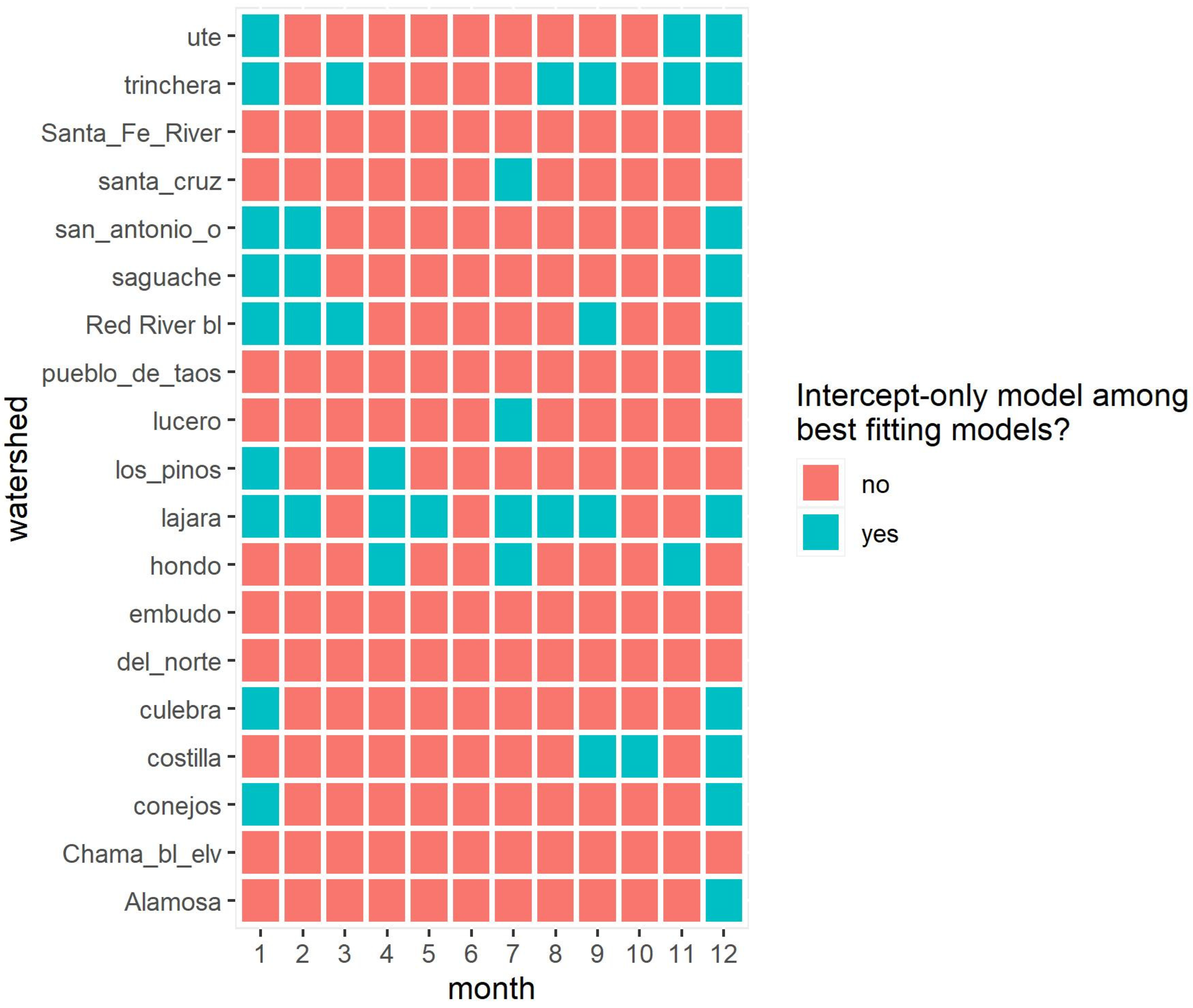
Intercept-Only Model

It is useful to identify which month(s) and watershed(s) cannot be effectively modeled by the candidate variables. Figure 6 shows “intercept-only” month and watershed combinations where the intercept-only model (flat line regression model) is among the best-fitting models.
The intercept-only model is never among the best fitting models for the Santa Fe River, Embudo, Del Norte, and Chama sub-watersheds. However, for the La Jara sub watershed, it is the best fitting model for the majority of months of the year, and for the Trinchera, the intercept-only model is the best fitting for half of the year.

3.3. Model with 120 Different Orders

Since changing the priority order ranking influences the results, we ran models for a total of 120 possible orders to accommodate new rankings of the five variables and averaged the results (Figure 7).
There are several combinations of months and basins where SWE and sublimation are omitted because they have too many zeros. Therefore, the permutations of the rankings are excluded when SWE or sublimation was the top variable. Some parameter estimates are removed where the intercept-only model is one of the top models. SWE is the most influential predictor variable, followed by minimum temperature, precipitation, sublimation, and then soil moisture.

3.4. Interpretation

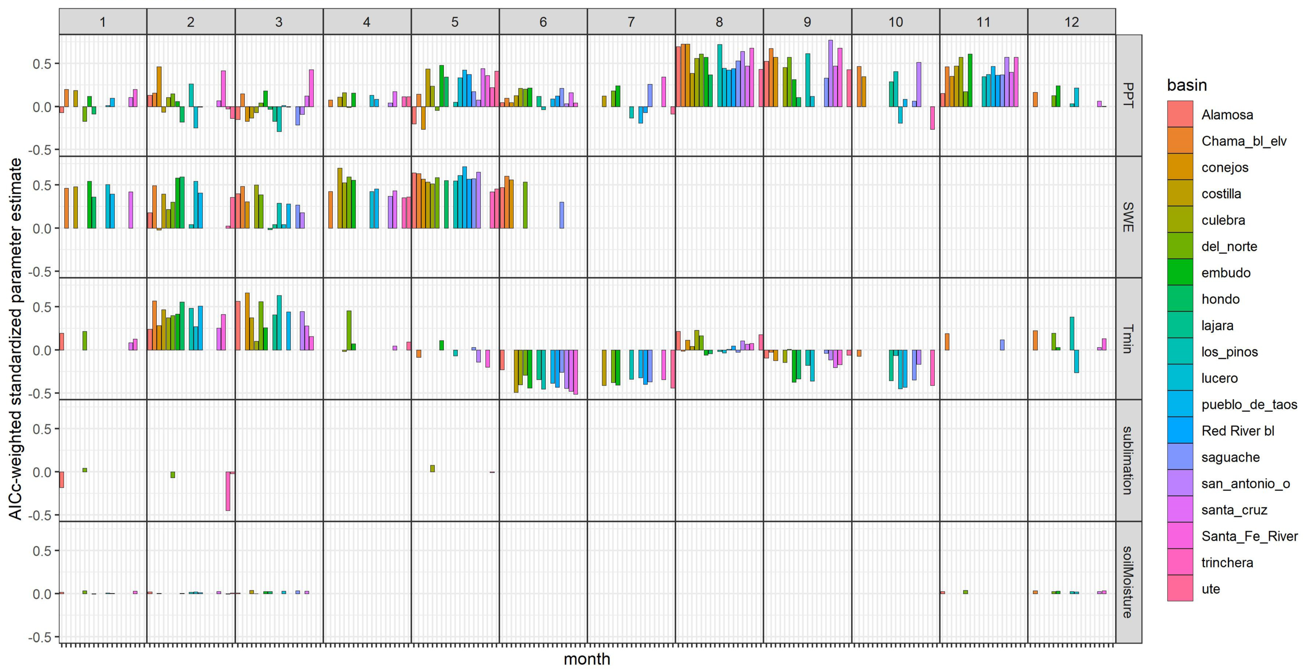
3.4.1. Interpretation by Predictor Variables

Precipitation—From January to April, the influence of precipitation is highly variable between watersheds. In May, it becomes positively related to streamflow for most of the watersheds, but this relationship is diminished in June and July when the influence of minimum temperature becomes more important. Precipitation has the strongest influence on streamflow in August, September, and November. This influence is mitigated somewhat in October (and September for some watersheds) by minimum temperature, likely due to the onset of freezing conditions. In May, precipitation is positively correlated with streamflow for most of the watersheds, but this relationship gradually diminishes in June and July when the influence of minimum temperature is more important. A few anomalies are identified in the results which are difficult to interpret. For instance, a very strong effect of precipitation was found from August to November. It is positively correlated in August and September, becomes negative in some sub-watersheds (Trinchera and Rio Lucero) in October, and returns to positive in November (Figure 7).
Soil Moisture—The relationship of soil moisture with streamflow is positive for the entire year but is relatively small compared to other variables.
Sublimation—The effect of sublimation gradually transitions from zero from July to December. However, there is some variability in effect between watersheds in the remaining months. In March, sublimation starts to have a negative relationship with streamflow; however, it becomes positive in some watersheds in May and June. The effect of sublimation in summer months is separately shown in Appendix B.
SWE—The influence of SWE is uniformly positive but is missing for several watersheds in many months. Lower elevation may account for this. The influence of SWE in summer months are illustrated in Appendix B.
Minimum Temperature—Temperature has the most interesting pattern. Warmer conditions in February and March tend to produce more streamflow, whereas warmer conditions in June, July, and October produce less streamflow. Its importance in August and September is mitigated by precipitation at the height of the monsoon.

3.4.2. Interpretation by Mountain Range

Figure 8 illustrates correlations of the predictor variables with streamflow in three different mountain ranges (Southern San Juan, Central Sangre De Cristo, and Southern Sangre De Cristo).
Precipitation is positively correlated with streamflow for the entire year for the Central Sangre De Cristo Mountain range and varies for the other mountain ranges. SWE also shows variability between the mountain ranges. SWE has no association with streamflow in the warming period between July and September for the Central Sangre De Cristo and the Southern Sangre De Cristo. SWE shows some association with streamflow during the warming period in the Southern San Juan range. This can be attributed to the altitude and geographic location of the Southern San Juan Mountain range.

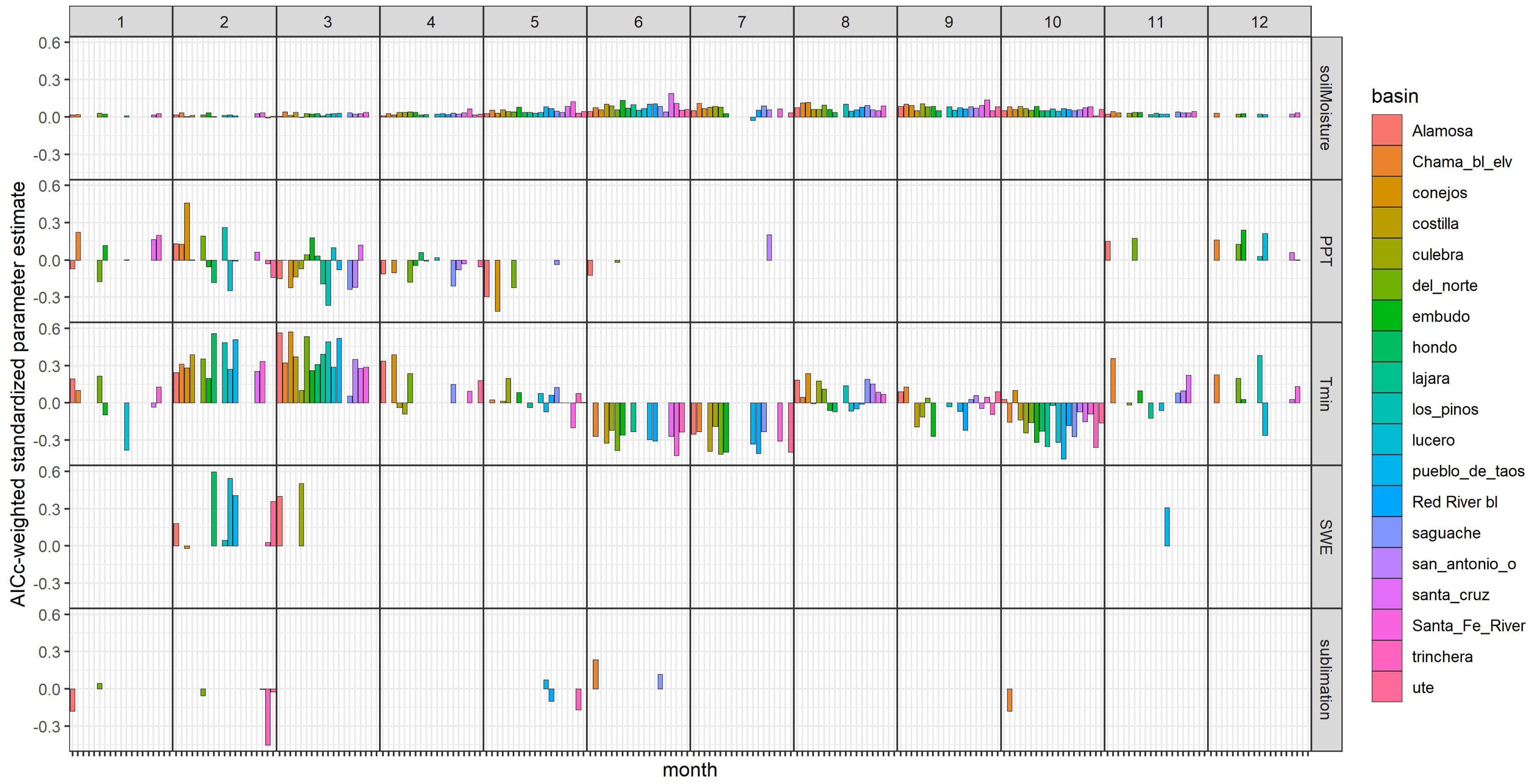
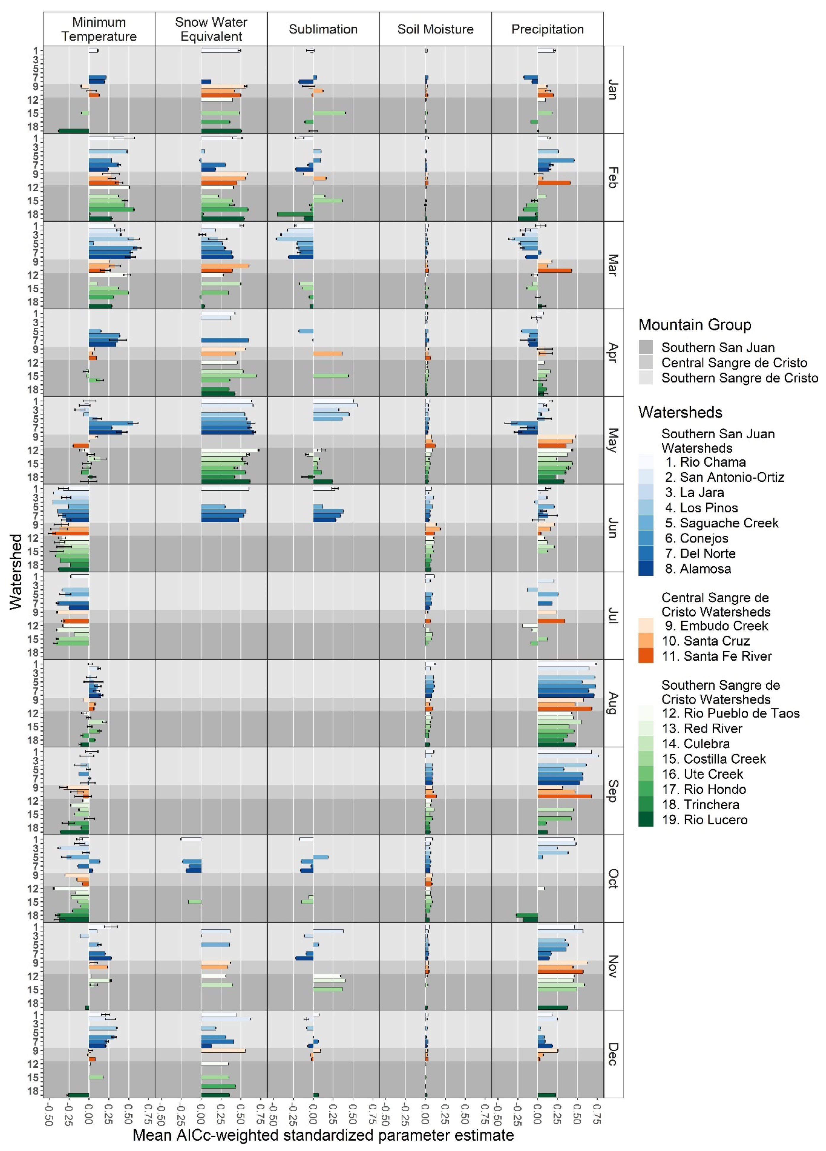
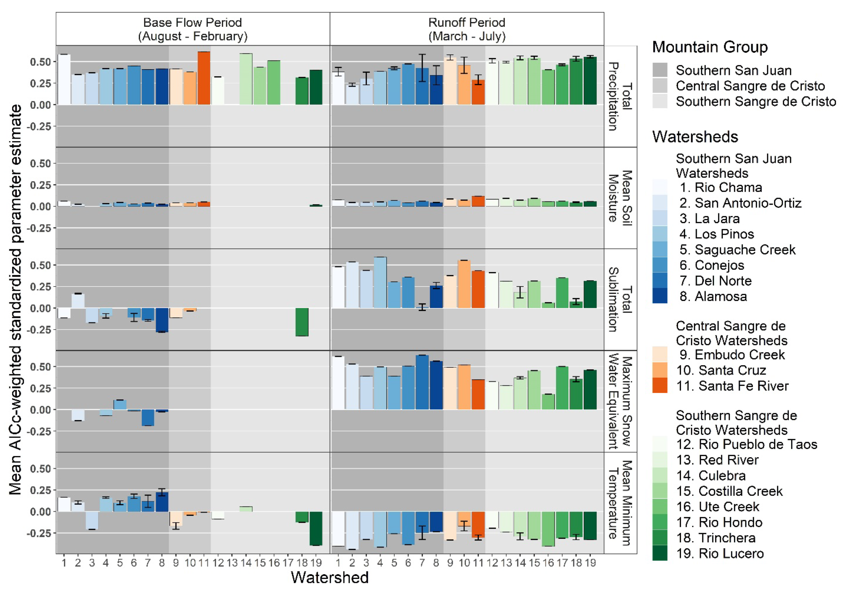
3.5. Estimation of Parameters by Period

We also calculate annual responses as the mean (soil moisture, minimum temperature), sum (precipitation, sublimation), and maximum (SWE) of the monthly responses. We evaluate the responses for runoff and base flow period. The following Table 3 described the aggregation method against each predictor variable.
Next, we run Pearson’s correlation with naturalized streamflow (Figure 9).
Figure 9 indicates a strong correlation between soil moisture and naturalized streamflow in the runoff season. The impact of precipitation on the naturalized streamflow is evident during base flow conditions. The associations with other variables such as sublimation, SWE, and minimum temperature vary by sub-watershed in both seasons. The association between mean minimum temperature and streamflow is negative for all watersheds during runoff season, whereas it is positive or statistically less during the baseflow period.

3.5.1. Interpretation by Variables and Watershed

Important variables are further investigated for annual streamflow estimation by generating regression equations and analyzing the goodness of fit using AICc-weighted standardized parameter estimates based on a 0.4 bivariate correlation cut off, adjusted for intercept-only model (taking the overall average). Figure 10 shows the relative influence of the predictor five variables on streamflow. We reported those variables which have clear line/bar, and we excluded the zero or faint line.
Similar to monthly estimation, important variables are further investigated for annual streamflow estimation through generating regression equations and analyzing goodness of fit (i.e., AICc-weighted standardized parameter estimates based on a 0.4 bivariate correlation cut off, adjusted for intercept only model, taking overall average). The goal of the “overall average” (Figure 10) was to show the relative importance of the five variables when explored together on influencing streamflow.
Precipitation is the most influential variable for normalized streamflow. SWE, temperature, and sublimation are also influential for normalized streamflow, especially during the runoff season, but they exhibit more temporal and spatial variability (Figure 10). The impact of precipitation on streamflow is consistent in each period for all watersheds across the basin. This trend is even more evident during the base flow period from August to February. Mean soil moisture is the least influential variable. It has a correlation coefficient greater than 0.4 with at least one of the other variables in each period for all watersheds. Therefore, we discarded this variable from the candidate model set in the periodical analysis. Mean minimum temperature is negatively correlated with streamflow during the runoff season. Mean minimum temperature varies for different sub-watersheds during the base flow period. Higher streamflow is observed with lower minimum temperatures from March to July for all watersheds. This occurrence might be due to less evapotranspiration with lower temperatures.
Maximum SWE is an influential variable during the runoff period. The influence of SWE varies for different watersheds in the baseflow period. Total Sublimation demonstrates a positive association with total stream flow within most sub-watersheds in the runoff season. A possible explanation may be that increasing concentrations of dust and dry and warm weather conditions accelerate sublimation and snowmelt runoff in the watersheds. Parameters are tabulated (Table 4) using their priority rank (1–4). Rank 1 indicates the most influential variable. For example, the most influential variable for Rio Chama during Baseflow is total precipitation. Different colors indicate different mountain ranges: Southern San Juan (blue), Central Sangre De Cristo (orange), and Southern Sangre De Cristo (green) in the Table 4.

3.5.2. Interpretation by Mountain Range and Season

Stream flow is largely dependent upon precipitation for all mountain groups throughout the year. During baseflow, precipitation is the most influential variable, with minimal influence from other variables. Precipitation, SWE, sublimation, and minimum temperature are all influential on streamflow during the runoff season for all mountain ranges.
SWE, sublimation, and minimum temperature have some influence on streamflow during baseflow in the Southern San Juan Mountains. This is due in part to the higher elevation of the mountain range in the northern part of the study area. SWE, sublimation, and minimum temperature have no influence on streamflow during baseflow in the Southern Sangre de Cristo Mountains. The exception is the Rio Lucero sub-watershed which is located at the highest elevation in the Southern Sangre de Cristo Mountains. Precipitation is the dominant influence on stream flow in the Central Sangre de Cristo Mountains. SWE and minimum temperature have minimal to nominal influence on streamflow in the Central Sangre de Cristo Mountains.

3.6. Discussion

An exploratory approach was taken in this article; we framed the analysis as an inquiry into variable influence ranking. Five predictor variables were primarily identified in order of relative importance as influential for streamflow prediction. The entire study was conducted from two different temporal angles, i.e., monthly analysis and seasonally by baseflow/runoff period. We retained important variables for streamflow through AICc-weighted standardized parameter estimates and model averaging parameter estimates based on ±0.4 bivariate correlation cut off; the equations were generated through multiple linear regression (MLR). We accounted for model uncertainty by employing an intercept-only model in each candidate model set.
The results can be reproduced by integrating future hydrologic data of the study area; variable influences can be monitored from time to time under regional climate change scenarios. This methodology can be replicated in other snowmelt-dominated regions for watershed monitoring and assessment.

4. Conclusions

This study explores the influence of candidate predictor variables on naturalized streamflow in nineteen sub-watersheds of the URG basin. Our results indicate that the predictor variables have variable influences on streamflow, including temporally between months and river periods and spatially between sub-watersheds and mountain ranges. Despite the importance of temperature on streamflow, it is not consistently the most important factor in streamflow prediction across time and space. The dominance of precipitation over streamflow is more obvious during baseflow. The impact of precipitation, SWE, sublimation, and minimum temperature on streamflow is evident during the runoff season, but the results vary for different sub-watersheds. The association between sublimation and streamflow is positive in the runoff season, which may relate to temperature and requires further research.
We explore variables fundamental to streamflow generation, leading to a variety of local water management implications i.e., modeling, monitoring, etc., in the face of climate change in the Upper Rio Grande. The research sheds light on the primary drivers and their spatial and temporal variability on streamflow generation. This research on surface water hydrology in the URG basin describes various statistics of parameter importance, identifying the main drivers in variable naturalized streamflow. This work is critical for predicting how warming temperatures will impact water supplies serving society and ecosystems in a changing climate. This research holds implications for better understanding a natural resource critical to the needs of society and a range of ecosystem services.

Supplementary Materials

The following supporting information can be downloaded at: https://www.mdpi.com/article/10.3390/rs14236076/s1.

Author Contributions

Conceptualization, K.I.I., E.E. and D.J.; Methodology, K.I.I., D.J.; Formal analysis, K.I.I.; Investigation, K.I.I. and E.E.; Resources, C.B.; Writing—original draft, K.I.I.; Writing—review & editing, S.H.; Supervision, C.B.; Funding acquisition, E.E. All authors have read and agreed to the published version of the manuscript.

Funding

The authors thank the U.S. Department of Agriculture—Agricultural Research Service (grant number #: 58-3050-9-012) and the Southwest Climate Hub for funding this research.

Acknowledgments

The Jornada Experimental Range (JER) at New Mexico State University deserves due appreciation for their support to the investigators. We would like to extend special thanks to Caiti Steele, JER, for her provision of time to help.

Conflicts of Interest

The authors declare no conflict of interest. The funders had no role in the design of the study; in the collection, analyses, or interpretation of data; in the writing of the manuscript; or in the decision to publish the results.

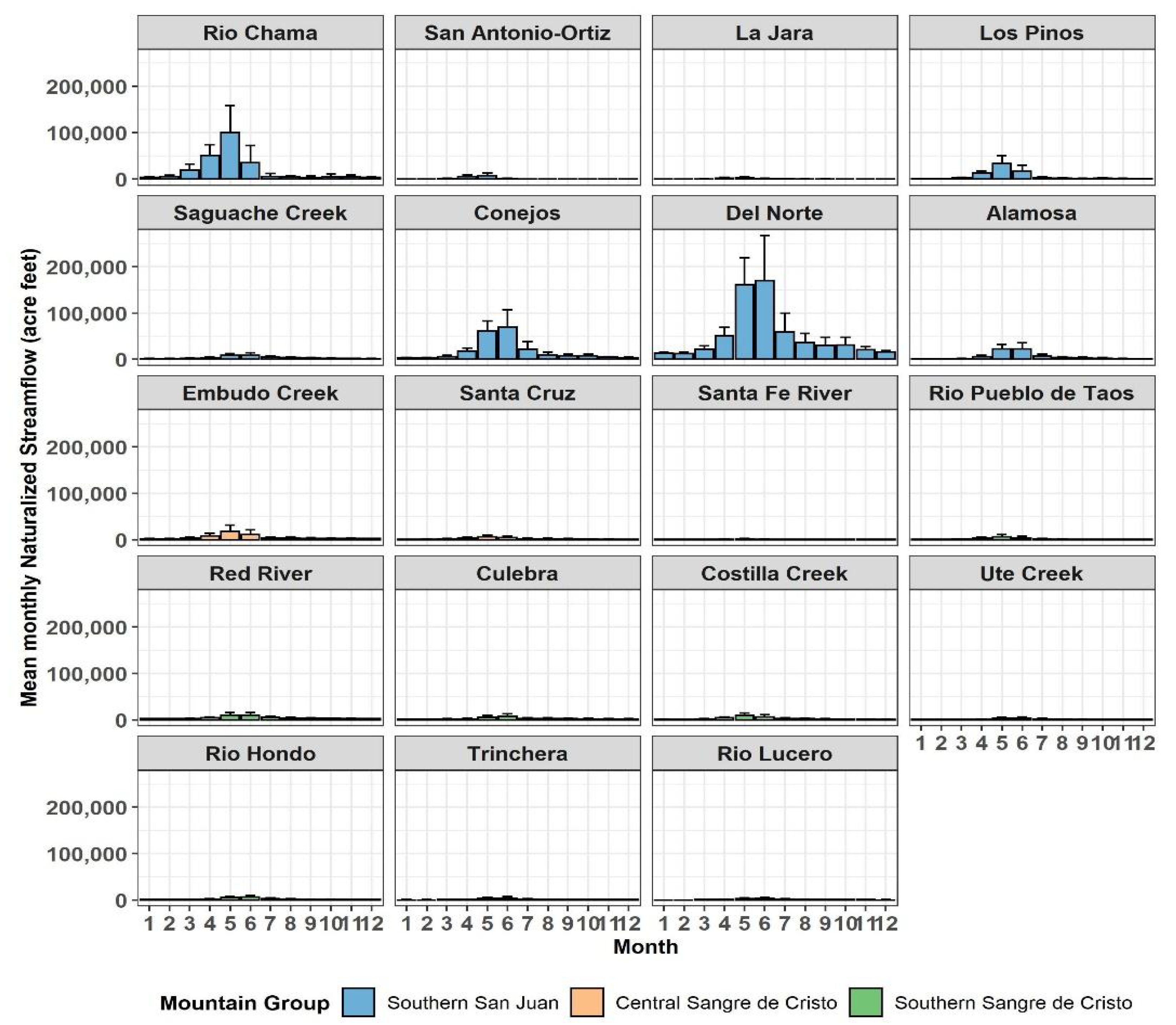
Appendix A. Monthly Mean Naturalized Streamflow for Each Sub Basin

We generated naturalized streamflow curves for each sub basin with the same y scale for each month in the following figure: it not only shows how naturalized stream flow varies monthly in watersheds but also it gives an idea over the volumetric distribution of the flow across the basin.
Figure A1. Monthly Mean Naturalized Streamflow.
Remotesensing 14 06076 g0a1

Appendix B. SWE and Sublimation in Summer Months

Here are two figures of SWE and sublimation that show annual patterns for each watershed. For reference, there are vertical lines in May and September. The months’ trends are not the same for each watershed. For example, the Santa Fe River tends to reach zero by May, while the Del Norte takes another month or two.
Figure A2. SWE in summer months.
Remotesensing 14 06076 g0a2
Figure A3. Sublimation in summer months.
Remotesensing 14 06076 g0a3

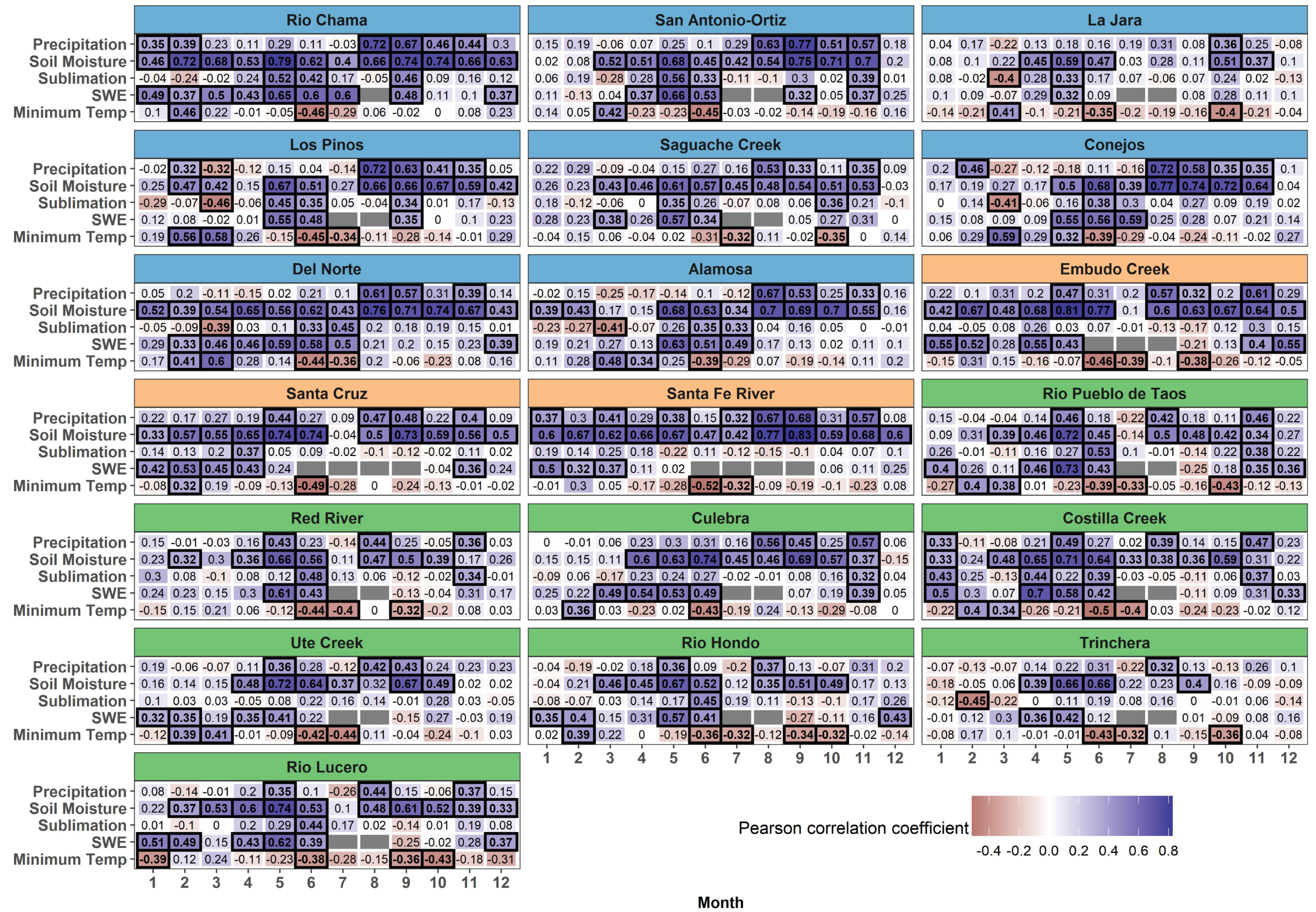
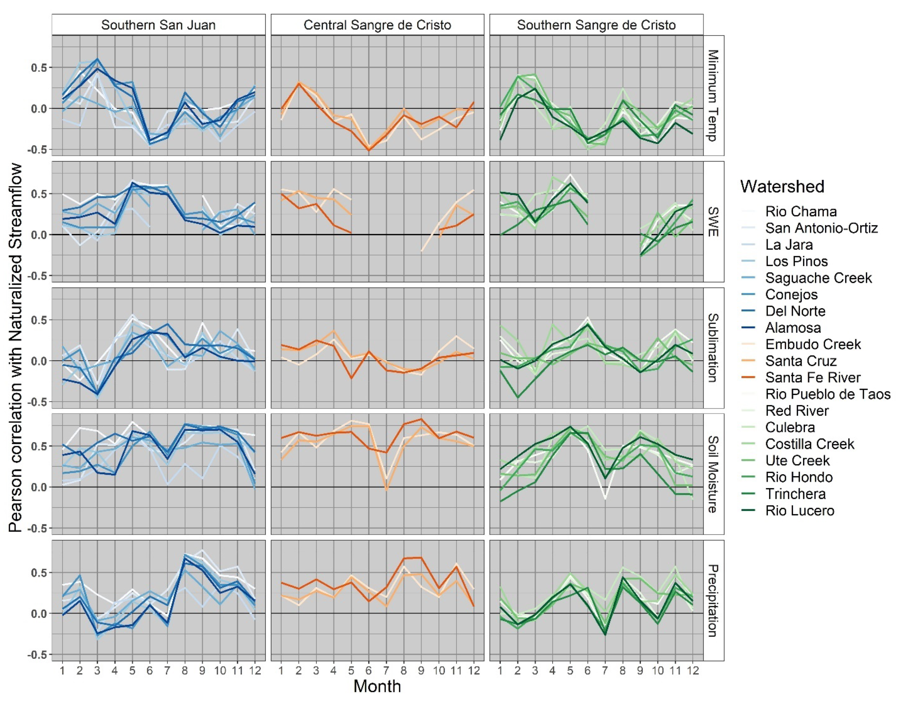
Appendix C. Pearson’s Correlation Coefficients with Naturalized Streamflow by Month

We calculated correlation coefficients particularly for each month to investigate how the relationships vary monthly. We estimated important parameters for the streamflow by separately exploring statistical models for monthly analysis.
Figure A4. Monthly correlation by sub watersheds of the URG basin.
Remotesensing 14 06076 g0a4

References

  1. Dettinger, M.; Udall, B.; Georgakakos, A. Western Water and Climate Change. Ecol. Appl. 2015, 25, 2069–2093. [Google Scholar] [CrossRef] [PubMed] [Green Version]
  2. Chavarria, S.B.; Gutzler, D.S. Observed Changes in Climate and Streamflow in the Upper Rio Grande Basin. JAWRA J. Am. Water Resour. Assoc. 2018, 54, 644–659. [Google Scholar] [CrossRef] [Green Version]
  3. Problem|WildEarth Guardians. Available online: http://www.rethinkingtherio.org/problem (accessed on 24 April 2022).
  4. The Vanishing Rio Grande: Warming Takes a Toll on a Legendary River. Available online: https://e360.yale.edu/features/warming-and-drought-take-a-toll-on-the-once-mighty-rio-grande (accessed on 23 September 2022).
  5. Garen, D.; Perkins, T.; Abramovich, R.; Julander, R.; Kaiser, R.; Lea, J.; McClure, R.; Tama, R. Snow Survey and Water Supply Forecasting; Water Supply Forecasting; Natural Resources Conservation Service, USDA: Washington, DC, USA, 2011; p. 25.
  6. U.S. Internation Boundary & Water Commission. Available online: https://www.ibwc.gov/crp/riogrande.htm (accessed on 21 September 2022).
  7. MacDonald, G.M. Water, Climate Change, and Sustainability in the Southwest. Proc. Natl. Acad. Sci. USA 2010, 107, 21256–21262. [Google Scholar] [CrossRef] [PubMed] [Green Version]
  8. Lehner, F.; Wahl, E.R.; Wood, A.W.; Blatchford, D.B.; Llewellyn, D. Assessing Recent Declines in Upper Rio Grande Runoff Efficiency from a Paleoclimate Perspective. Geophys. Res. Lett. 2017, 44, 4124–4133. [Google Scholar] [CrossRef]
  9. Fleming, S.W.; Vesselinov, V.V.; Goodbody, A.G. Augmenting Geophysical Interpretation of Data-Driven Operational Water Supply Forecast Modeling for a Western US River Using a Hybrid Machine Learning Approach. J. Hydrol. 2021, 597, 126327. [Google Scholar] [CrossRef]
  10. NRCS National Water and Climate Center—Publication—Water Supply Forecasts—A Field Office Guide for Interpreting Streamflow Forecasts—Section 2—Questions and Answers. Available online: https://www.wcc.nrcs.usda.gov/factpub/fcst_s2.htm (accessed on 3 April 2020).
  11. Zhang, Y.; Touzi, R.; Feng, W.; Hong, G.; Lantz, T.C.; Kokelj, S.V. Landscape-Scale Variations in near-Surface Soil Temperature and Active-Layer Thickness: Implications for High-Resolution Permafrost Mapping. Permafr. Periglac. Process. 2021, 32, 627–640. [Google Scholar] [CrossRef]
  12. Lehner, F.; Wood, A.W.; Llewellyn, D.; Blatchford, D.B.; Goodbody, A.G.; Pappenberger, F. Mitigating the Impacts of Climate Nonstationarity on Seasonal Streamflow Predictability in the U.S. Southwest. Geophys. Res. Lett. 2017, 44, 12208–12217. [Google Scholar] [CrossRef] [Green Version]
  13. Shultz, D. Snowpack Data Sets Put to the Test. Available online: https://doi.org/10.1029/2020EO141900 (accessed on 10 April 2020).
  14. Park, S.-E. Variations of Microwave Scattering Properties by Seasonal Freeze/Thaw Transition in the Permafrost Active Layer Observed by ALOS PALSAR Polarimetric Data. Remote Sens. 2015, 7, 17135–17148. [Google Scholar] [CrossRef] [Green Version]
  15. Touzi, R. Target Scattering Decomposition in Terms of Roll-Invariant Target Parameters. IEEE Trans. Geosci. Remote Sens. 2006, 45, 73–84. [Google Scholar] [CrossRef]
  16. Muhuri, A.; Manickam, S.; Bhattacharya, A. Snow Cover Mapping Using Polarization Fraction Variation with Temporal RADARSAT-2 C-Band Full-Polarimetric SAR Data over the Indian Himalayas. IEEE J. Sel. Top. Appl. Earth Obs. Remote Sens. 2018, 11, 2192–2209. [Google Scholar] [CrossRef]
  17. Gascoin, S.; Grizonnet, M.; Bouchet, M.; Salgues, G.; Hagolle, O. Theia Snow Collection: High-Resolution Operational Snow Cover Maps from Sentinel-2 and Landsat-8 Data. Earth Syst. Sci. Data 2019, 11, 493–514. [Google Scholar] [CrossRef] [Green Version]
  18. Kostadinov, T.S.; Schumer, R.; Hausner, M.; Bormann, K.J.; Gaffney, R.; McGwire, K.; Painter, T.H.; Tyler, S.; Harpold, A.A. Watershed-Scale Mapping of Fractional Snow Cover under Conifer Forest Canopy Using Lidar. Remote Sens. Environ. 2019, 222, 34–49. [Google Scholar] [CrossRef]
  19. US EPA Office. A Closer Look: Temperature and Drought in the Southwest. Available online: https://www.epa.gov/climate-indicators/southwest (accessed on 22 September 2022).
  20. Elias, E.H.; Rango, A.; Steele, C.M.; Mejia, J.F.; Smith, R. Assessing Climate Change Impacts on Water Availability of Snowmelt-Dominated Basins of the Upper Rio Grande Basin. J. Hydrol. Reg. Stud. 2015, 3, 525–546. [Google Scholar] [CrossRef]
  21. US EPA Office. Climate Change Indicators: Snow Cover. Available online: https://www.epa.gov/climate-indicators/climate-change-indicators-snow-cover (accessed on 22 September 2022).
  22. Qiao, D.; Li, Z.; Zhang, P.; Zhou, J.; Liang, S. Prediction of Snow Depth Based on Multi-Source Data and Machine Learning Algorithms. In Proceedings of the 2021 IEEE International Geoscience and Remote Sensing Symposium IGARSS, Brussels, Belgium, 11–16 July 2021; pp. 5578–5581. [Google Scholar]
  23. Schneider, D.; Molotch, N.P. Real-Time Estimation of Snow Water Equivalent in the U Pper C Olorado R Iver B Asin Using MODIS-Based SWE Reconstructions and SNOTEL Data. Water Resour. Res. 2016, 52, 7892–7910. [Google Scholar] [CrossRef]
  24. Meyal, A.Y.; Versteeg, R.; Alper, E.; Johnson, D.; Rodzianko, A.; Franklin, M.; Wainwright, H. Automated Cloud Based Long Short-Term Memory Neural Network Based SWE Prediction. Front. Water 2020, 2, 574917. [Google Scholar] [CrossRef]
  25. Sexstone, G.A.; Driscoll, J.M.; Hay, L.E.; Hammond, J.C.; Barnhart, T.B. Runoff Sensitivity to Snow Depletion Curve Representation within a Continental Scale Hydrologic Model. Hydrol. Process. 2020, 34, 2365–2380. [Google Scholar] [CrossRef]
  26. Landry, C.; Buck, K. Dust-on-Snow Effects on Colorado Hydrographs. In Proceedings of the Western Snow Conference 2014, Durango, Colorado, 14–17 April 2014; p. 6. [Google Scholar]
  27. Goldstein, H.L.; Reynolds, R.L.; Landry, C.; Derry, J.E.; Kokaly, R.F.; Breit, G.N. The Effects of Dust on Colorado Mountain Snow Cover Albedo and Compositional Links to Dust-Source Areas. AGU Fall Meet. Abstr. 2016, 2016, A21E-0106. [Google Scholar]
  28. Lapp, S.; Byrne, J.; Townshend, I.; Kienzle, S. Climate Warming Impacts on Snowpack Accumulation in an Alpine Watershed. Int. J. Climatol. 2005, 25, 521–536. [Google Scholar] [CrossRef]
  29. Painter, T.H.; Skiles, S.M.; Deems, J.S.; Bryant, A.C.; Landry, C.C. Dust Radiative Forcing in Snow of the Upper Colorado River Basin: 1. A 6 Year Record of Energy Balance, Radiation, and Dust Concentrations. Water Resour. Res. 2012, 48, W07521. [Google Scholar] [CrossRef] [Green Version]
  30. Milly, P.C.D.; Dunne, K.A. Colorado River Flow Dwindles as Warming-Driven Loss of Reflective Snow Energizes Evaporation. Science 2020, 367, 1252–1255. [Google Scholar] [CrossRef]
  31. Cooley, E.; Frame, D.; Wunderlin, A. Soil Moisture and Potential for Runoff. 2010, p. 6. Available online: https://uwdiscoveryfarms.org/UWDiscoveryFarms/media/sitecontent/PublicationFiles/farmpagel/Soil-Moisture-and-Potential-for-Runoff-factsheet.pdf?ext=.pdf (accessed on 28 October 2020).
  32. USA Detailed Streams. Available online: https://www.arcgis.com/home/item.html?id=1e29e33360c8441bbb018663273a046e (accessed on 30 January 2021).
  33. ArcGIS 10 (Desktop, Engine, Server) Service Pack 5—English. Available online: https://support.esri.com/en/download/1876 (accessed on 2 July 2022).
  34. Gesch, D.B.; Evans, G.A.; Oimoen, M.J.; Arundel, S. The National Elevation Dataset; American Society for Photogrammetry and Remote Sensing: Baton Rouge, LA, USA, 2018; pp. 83–110. [Google Scholar]
  35. USGS Current Water Data for the Nation. Available online: https://waterdata.usgs.gov/nwis/rt (accessed on 24 April 2022).
  36. Loeser, C.; Rui, H.; Teng, W.; Vollmer, B.; Mocko, D. Enabling NLDAS-2 Anomaly Analysis Using Giovanni. In Proceedings of the AGU 2017 Fall Meeting H21F-1558, New Orleans, LA, USA, 11–15 December 2017. [Google Scholar]
  37. MODIS/Terra Snow Cover Monthly L3 Global 0.05Deg CMG, Version 6|National Snow and Ice Data Center. Available online: https://nsidc.org/data/mod10cm/versions/6 (accessed on 3 August 2022).
  38. PRISM Climate Group, Oregon State U. Available online: http://www.prism.oregonstate.edu/historical/ (accessed on 5 June 2020).
  39. DATA ACCESS-SMERGE Version 2.0. Available online: https://www.tamiu.edu/cees/smerge/data.shtml (accessed on 5 June 2020).
  40. GES DISC Dataset: NLDAS Mosaic Land Surface Model L4 Monthly 0.125 × 0.125 Degree V002 (NLDAS_MOS0125_M 002). Available online: https://disc.gsfc.nasa.gov/datasets/NLDAS_MOS0125_M_002/summary (accessed on 23 September 2022).
  41. NRCS National Water and Climate Center|Home. Available online: https://www.wcc.nrcs.usda.gov/about/forecasting.html (accessed on 3 April 2020).
  42. NLDAS Mosaic Land Surface Model L4 Monthly 0.125 × 0.125 Degree V002 (NLDAS_MOS0125_M) at GES DISC. Available online: https://cmr.earthdata.nasa.gov/search/concepts/C1233767610-GES_DISC.html (accessed on 23 September 2022).
  43. Data Catalogues. Available online: https://jornada.nmsu.edu/data-catalogs (accessed on 15 June 2020).
  44. RStudio|Open Source & Professional Software for Data Science Teams—RStudio. Available online: https://www.rstudio.com/ (accessed on 22 September 2022).
  45. Goodbody, A. Stream Flow Data 2020. Unpunlished work.
  46. Water Supply Forecasts—A Field Office Guide for Interpreting Streamflow Forecasts—Section 1—Narrative. Available online: https://www.wcc.nrcs.usda.gov/factpub/fcst_s1.htm (accessed on 3 April 2020).
  47. Mazerolle, M.J. AICcmodavg. R Package; Version 2.3-1; The R Foundation: Vienna, Austria, 2020; Available online: https://cran.r-project.org/web/packages/AICcmodavg/AICcmodavg.pdf (accessed on 11 November 2021).
  48. Mazerolle, M.J. Model Selection and Multimodel Inference Using the AICcmodavg Package 2020. Available online: https://cran.r-project.org/web/packages/AICcmodavg/vignettes/AICcmodavg.pdf (accessed on 11 November 2021).
  49. Burnham, K.P.; Anderson, D.R.; Burnham, K.P. Model Selection and Multimodel Inference: A Practical Information-Theoretic Approach, 2nd ed.; Springer: New York, NY, USA, 2002; ISBN 978-0-387-95364-9. [Google Scholar]
  50. Anderson, D.; Burnham, K. Model Selection and Multi-Model Inference, 2nd ed.; Springer: New York, NY, USA, 2004; Volume 63, p. 10. [Google Scholar]
  51. Cade, B.S. Model Averaging and Muddled Multimodel Inferences. Ecology 2015, 96, 2370–2382. [Google Scholar] [CrossRef] [PubMed] [Green Version]
  52. Al-Samman, E.N. The Influence of Transparency on the Leaders’ Behaviors. Master’s Thesis, Open University Malaysia (OUM), Petaling Jaya, Malaysia, 2012. [Google Scholar]
Figure 1. (A) Study Region: The study watersheds and streamlines, (B) Elevation Map: The URG basin.
Remotesensing 14 06076 g001
Figure 2. Clipped area in ArcMap (upper right) and R (lower right).
Remotesensing 14 06076 g002
Figure 3. Procedural Flowchart of the analytical process.
Remotesensing 14 06076 g003
Figure 4. AICc-weighted standardized parameter estimates based on ± 0.4 bivariate correlation cut-off, adjusted for intercept-only model. The priority ranking is: 1. Precipitation, 2. Soil Moisture, 3. Sublimation, 4. SWE, and 5. Minimum Temperature.
Remotesensing 14 06076 g004
Figure 5. AICc-weighted standardized parameter estimates based on ± 0.4 bivariate correlation cut off, adjusted for intercept-only model. The priority ranking is: 1. Soil Moisture, 2. Precipitation, 3. Minimum Temperature, 4. SWE, and 5. Sublimation.
Remotesensing 14 06076 g005
Figure 6. “Intercept-only” model for month and watershed combinations.
Remotesensing 14 06076 g006
Figure 7. AICc-weighted standardized parameter estimates, adjusted with intercept-only models.
Remotesensing 14 06076 g007
Figure 8. Line plots of monthly correlation of the variables with streamflow.
Remotesensing 14 06076 g008
Figure 9. Pearson’s correlation coefficients with naturalized streamflow for subbasins of the Upper Rio Grande. Outline indicates significance at p = 0.05, color indicates positive or negative correlation, and shade corresponds with x.
Remotesensing 14 06076 g009
Figure 10. Overall average of estimation of parameter by period, with AICc-weighted standardized parameter estimates.
Remotesensing 14 06076 g010
Table 1. Nineteen sub-watersheds in the URG basin and their associated USGS gauging station number, basin area, and elevation range.
USGS Gauging
Station
Basin Area (sq-km)Elevation Range (m.a.s.l)
Alamosa082360002742624–4036
Conejos082465007292524–4005
Costilla Creek082555005662409–3941
Culebra082500006492428–4265
Del Norte0822000033962436–4222
Embudo Creek082790008281787–3912
La Jara082380002662464–3632
Los Pinos082480003952454–3716
Red River below Fish Hatchery near Questa082668202902276–3988
Rio Chama below el Vado dam0828550012222159–3886
Rio Hondo08267500962349–3992
Rio Lucero08271000432472–3976
Rio Pueblo de Taos082690001502262–3892
Saguache Creek0822700013402448–4229
San Antonio-Ortiz082475002982437–3327
Santa Cruz082910002391974–3972
Santa Fe River08316000472368–3757
Trinchera082405001372601–4113
Ute Creek082425001042459–4351
Table 2. Variables used in the study and their respective data format and sources.
VariablesType of DataUnitSource/Organization
Snow-water Equivalent (SWE)Raster: monthly meanKg/m2Goddard Earth Sciences Data and Information Services Center, or GES DISC—National Aeronautics and Space Administration (NASA) [36]
Snow coverRaster: monthly meanFractionModerate Resolution Imaging Spectroradiometer (MODIS)—National Aeronautics and Space Administration (NASA) [37]
TemperatureRaster: monthly mean
and minimum
Celsius (°C)Parameter-elevation Regression on Independent Slopes Model (PRISM) [38]
PrecipitationRaster: monthly meanmmParameter-elevation Regression on Independent Slopes Model (PRISM) [38]
SublimationRaster: monthlyWatt/m2Goddard Earth Sciences Data and Information Services Center, or GES DISC—National Aeronautics and Space Administration (NASA) [39,40]
Naturalized Streamflow Hydrograph Monthly VolumeAc-ftNatural Resources Conservation Service (NRCS) [41]
Soil MoistureRaster: monthlyKg/m2Center for Earth and Environmental Studies, Texas A & M International University [39]
Snow DepthRaster: monthlyMeter (m)Goddard Earth Sciences Data and Information Services Center, or GES DISC—National Aeronautics and Space Administration (NASA) [39,40]
Snow AlbedoRaster Monthly%Goddard Earth Sciences Data and Information Services Center, or GES DISC—National Aeronautics and Space Administration (NASA) [39,42]
Stream LayerFeatureN/AESRI—Environmental Systems Research Institute [32]
Basin BoundaryFeatureN/AUSDA Southwest Climate Hub, Jornada Experimental Range (JER) [43]
Table 3. The data aggregation method for seasonal analysis.
VariableAggregation Method
Naturalized StreamflowSummation of each month of the season
Snow Water Equivalent (SWE)Monthly Maximum for the season
Soil MoistureSeasonal average
PrecipitationSummation of each month of the season
SublimationSummation of each month of the season
Minimum Temperature Seasonal average
Table 4. Important Parameters along with their ranks for each of the 19 watersheds.
Important Variables
Rank of the Parameters: Baseflow PeriodRank of the Parameters: Runoff Period
Rank1 Rank2Rank3Rank4Rank1 Rank2Rank3Rank 4
Rio ChamaTotal PrecipitationMean Min. Temp.Total Sublimation Maximum SWETotal SublimationMean Min. Temp.Total Precipitation
San AntonioTotal PrecipitationTotal SublimationMaximum SWEMean Min. Temp.Total SublimationMaximum SWEMean Min. Temp.Total Precipitation
La JaraTotal PrecipitationMean Min. Temp.Total Sublimation Total SublimationMaximum SWEMean Min. Temp.Total Precipitation
Los PinosTotal PrecipitationMean Min. Temp. Max. SWETotal SublimationMaximum SWEMean Min. Temp.Total Precipitation
Saguache CreekTotal PrecipitationMax. SWEMean Min. Temp. Total PrecipitationMaximum SWETotal SublimationMean Min. Temp.
ConejosTotal PrecipitationMean Min. Temp.Total Sublimation Maximum SWETotal PrecipitationMean Min. Temp.Total Sublimation
Del NorteTotal PrecipitationMax. SWETotal SublimationMean Min. Temp.Maximum SWETotal PrecipitationMean Min. Temp.
AlamosaTotal PrecipitationTotal SublimationMean Min. Temp. Maximum SWETotal PrecipitationTotal SublimationMean Min. Temp.
Embudo CreekTotal PrecipitationMean Min. Temp.Total Sublimation Total PrecipitationMaximum SWETotal SublimationMean Min. Temp.
Santa CruzTotal Precipitation Total SublimationMaximum SWETotal PrecipitationMean Min. Temp.
Santa Fe RiverTotal Precipitation Total SublimationMaximum SWETotal PrecipitationMean Min. Temp.
Rio Pueblo de_taosNo variable Total PrecipitationTotal SublimationMaximum SWEMean Min. Temp.
Red RiverTotal Precipitation Total PrecipitationTotal SublimationMaximum SWEMean Min. Temp.
CulebraTotal Precipitation Total PrecipitationMaximum SWEMean Min. Temp.Total Sublimation
Costilla CreekTotal Precipitation Total PrecipitationMaximum SWEMean Min. Temp.Total Sublimation
Ute CreekTotal Precipitation Total PrecipitationMaximum SWEMean Min. Temp.Total Sublimation
Rio HondoTotal Precipitation Maximum SWETotal PrecipitationTotal SublimationMean Min. Temp.
TrincheraTotal Precipitation Maximum SWETotal SublimationTotal PrecipitationMean Min. Temp.
Total Precipitation Maximum SWETotal SublimationTotal PrecipitationMean Min. Temp.
Publisher’s Note: MDPI stays neutral with regard to jurisdictional claims in published maps and institutional affiliations.

