The Coupling of Glacier Melt Module in SWAT+ Model Based on Multi-Source Remote Sensing Data: A Case Study in the Upper Yarkant River Basin

Abstract

Glaciers have proven to be a particularly sensitive indicator of climate change, and the impacts of glacier melting on downstream water supplies are becoming increasingly important as the world’s population expands and global warming continues. Data scarcity in mountainous catchments, on the other hand, has been a substantial impediment to hydrological simulation. Therefore, an enhanced glacier hydrological model combined with multi-source remote sensing data was introduced in this study and was performed in the Upper Yarkant River (UYR) Basin. A simple yet efficient degree-day glacier melt algorithm considering solar radiation effects has been introduced for the Soil and Water Assessment Tool Plus model (SWAT+), sensitivity analysis and auto calibration/validation processes were integrated into this enhanced model as well. The results indicate that (i) including glacio-hydrological processes and multi-source remote sensing data considerably improved the simulation precision, with a Nash–Sutcliffe efficiency coefficient (NSE) promotion of 1.9 times and correlated coefficient (R²) of 1.6 times greater than the original model; (ii) it is an efficient and feasible way to simulate glacio-hydrological processes with SWAT+Glacier and calibrate it using observed discharge data in data-scarce and glacier-melt-dominated catchments; and (iii) glacier runoff is intensively distributed throughout the summer season, accounting for about 78.5% of the annual glacier runoff, and glacier meltwater provides approximately 52.5% (4.4 × 10⁹ m³) of total runoff in the study area. This research can serve the runoff simulation in glacierized regions and help in understanding the interactions between streamflow components and climate change on basin scale.

1. Introduction

The evaluation of hydro-climatic change and hydrological modeling in alpine and glacierized catchments are both fraught with uncertainty and complexity. Field observations for hydrological components such as glaciers, snow cover, and permafrost at the basin scale are frequently limited due to high altitude, complex geography, and atmospheric conditions. Glaciers have drawn remarkable attention for two primary reasons. The first is that they keep a considerable quantity of freshwater, which is crucial for downstream agriculture, industrial activities, and living beings. Another reason is that, as one of the most sensitive indicators of global warming, many alpine glaciers worldwide are experiencing a continuously rapid shrinkage and thinning [1,2,3], along with various associated natural hazards such as ice/snow avalanches, glacial lake outburst flood (GLOF), debris flow, landslides, which has significantly affected facilities and living beings downstream during recent decades. As a result, glacio-hydrological processes must be included in hydrological research for these glacierized watersheds.

Meanwhile, the strength and predictive abilities of hydrological model are heavily reliant on the input data including topography, land use, and climate [4]. Data scarcity has always been a key challenge for gaining a thorough knowledge understanding of complicated hydrological processes that occur in alpine locations, necessitating the use of simple and efficient glacier modeling algorithms. As a result of limited physical access to the alpine and remote regions, large-coverage satellite imageries are becoming the predominant data source used to monitor the temperature and precipitation change in these unique environments. Reanalysis datasets, multi-source merged datasets, and satellite remote sensing data are widely used in climate change research [5]. Climate data with good quality, especially accurate precipitation information, is crucial for climate change models, as well as hydrological simulations, disaster risks mitigations, and agricultural management [6,7,8].

In recent years, a considerable number of glacier studies both focused on the single glacier and regional scales have been undertaken using observation data, remote sensing images, and model simulation findings [9,10,11,12,13,14]. A growing number of hydrological models have been developed and applied to examine the link between glacier streamflow and climate change. For example, to improve model performance in the Aksu river basin, a coupled energy mass balance scheme based on the framework of the Variable Infiltration Capacity Macroscale Hydrologic Model (VIC) was utilized [15]. An integrated glacier dynamics module for a semi-distributed hydrological model SWIM (Soil and Water Integrated Model) by [16] was also developed and validated in data-scarce watersheds of the Upper Aksu River, Kyrgyzstan/NW China, and the relatively data-abundant Upper Rhone River, Switzerland. In addition, to better understand the impacts of glacier and snow on hydrological response, a modified degree-day algorithm was implemented into the Hydrologiska Byråns Vattenbalansavdelning (HBV) model [17] and demonstrated a good performance in the cold mountainous basins [18,19,20,21,22].

As illustrated above, in situ mass balance and glacier change data are only accessible for a limited number of glaciers and over quite short time periods [23]. As a result of these constraints, the snow and glacier hydrological processes incorporated into the hydrological model must address both efficient performance and easy data accessibility. For the simulation of glacier and snow dynamics, two fundamental techniques known as energy balance models and temperature-index models were often used in hydrological models [24,25,26]. Taking the calculation of glacier meltwater as an example, the former approach is a physically based model that computes it as the sum of all relevant energy fluxes, whereas the latter frequently considers it to be a product of air temperature and an empirical coefficient known as the degree-day factor, with air temperature serving as the single measurable input variable.

Soil and Water Assessment Tool (SWAT) is a semi-distributed hydrological model with a nearly 40-year history that has been proven to be one of the most widely used hydrological models and effective tools for water resource evaluation globally [4,27,28,29,30]. Though glacier hydrology process is not built-in, numerous researchers have attempted to include the classical degree-day model, a commonly used glacier melt algorithm across the world due to its low data requirement, into this model [16,31,32,33,34]. The enhanced temperature-index approach combined with solar radiation incorporated into SWAT has suggested a high performance in glacierized basins as well [35]. However, the application is usually restricted to the simulation of melt rates at a daily or coarser resolution, and in a lumped or semi-lumped manner for calculating average melt rates throughout an entire basin [36].

Over the last two decades, a number of constraints have been recognized, new functionalities have been introduced, and other changes have resulted in the code being more difficult to manage and maintain. To meet the needs of the growing global user community as well as the challenges of water resource modeling and management, the SWAT code has undergone major modifications in recent years, resulting in a completely revised version known as SWAT+, a far more flexible model than SWAT in terms of the spatial representation of interactions and processes within a watershed [37]. Despite the basic algorithms of the model remaining unchanged, the structure and organization of both the code and input/output files have been significantly altered, which is expected to facilitate model maintenance, future code modifications, and integration of new components into SWAT modules and algorithms. Nevertheless, the glacier hydrology process is not currently included in SWAT+ at present, which would result in severely inaccurate simulations in glacierized catchments.

This study intends to integrate an enhanced temperature-index glacier melt algorithm that considers the impact of solar radiation with SWAT+ model, allowing the glacier hydrology process to be simulated using multi-source remote sensing data as model inputs at glacierized basins.

2. Material and Methods

2.1. Description of SWAT+ Model

SWAT+ is a total redesigned version of SWAT that provides more flexibility and additional capabilities to facilitate model maintenance and code modifications [37]. Many aspects have been considerably enhanced, including watershed configuration, spatial connections, input/output file format, land use and management, constituents, and the calibration process. For instance, numerous input files have been reduced, the output file formats have been standardized, and can be printed at any user-defined time steps in SWAT+. Changes in parameter values stated in a separate calibration file result in a considerably speedier calibration experience and better monitoring of updated parameters.

Sub-basins in SWAT+ may be separated into landscape units (LSUs), and flow can be routed between these LSUs. Flow generated in the hydrological response units (HRUs) is aggregated at the LSU level and may be routed from the LSU to any other spatial object within the watershed to improve water transfer modeling at the watershed scale. Precipitation is separated into liquid and solid forms using a specific air temperature, which is normally taken as 0 °C and can be calibrated subsequently. The depletion curves are used to identify the area change of snow cover in an HRU, whereas the degree-day approach is used to estimate snowmelt.

To simulate the glacier hydrology process using SWAT+, especially the glacier melt process, glaciers must first be recognized at the HRU level, after which a dynamic glacier area approach and an extended glacier melt algorithm are implemented at the HRU level, which is provided in detail below.

2.2. Incorporation of Glacier Module

The incorporation of the glacier hydrological process into SWAT+ has been represented as the following framework (Figure 1). First, the glacierized part of the catchment was disaggregated into glaciological response units based on land use, soil, elevation zone and aspect classes and seamlessly integrated into the HRUs of the hydrological model. During this process, glacier boundaries derived from the Second Glacier Inventory of China [38,39] were introduced to the input land-use data to identify glacier HRUs as a specified land-use type. Then, modified snow process and added glacier process were invoked when a glacier HRU was recognized. For instance, water yield from snow and glacier melt in glacier HRUs were added into the efficient precipitation and then routed into channels to generate runoff, while sublimation of snow and glacier was considered as another loss of the water balance in glacier HRUs and used to update the remaining snow and glacier water content.

Finally, it should be noted that there are two main differences between the snow processes in a glacier HRU and a non-glacier HRU, which is that only in the former case turnover of snow to ice is considered and the glacier will be melted when the energy exceeds the amount of covered snow, individually.

The incorporated glacier algorithm is explained in detail as follows:

Glacier water equivalent depth ($W_g$, mm H₂O) during a certain time step (t, days) is often illustrated by the concept of glacier mass balance, which is the algebraic sum of the income and expenditure material of the glacier system and can be expressed as:

$$\frac{d{W}_g}{dt}=-\left(1-f\right)M-S+F$$

(1)

where M is the melt rate of ice in mm H₂O day⁻¹, $f$ is the ratio for meltwater refreezing, S is sublimation rate of ice in mm H₂O day⁻¹, F is glacier accumulation rate in mm H₂O day⁻¹. A dynamic glacier hydrological response unit scheme introduced by previous research [33] was applied to this paper to capture glacier changes. This method simply considers glacier mass balance as the sum of glacier melt, sublimation, and accumulation, an empirical formula of glacier volume–area relation was also conducted to adjust glacier water content and capture glacier change in HRU level, in which glacier HRUs were recognized with a predefined specific land use. The same procedure was conducted in our work, and snow processes were always calculated first in HRUs. In particular, when the energy exceeded the amount of the residual snow water equivalent (SWE), the snowmelt was considered as equal to the value of residual SWE, and no snow cover existed in this case for normal HRUs. However, when it was a glacier HRU and the air temperature exceeded glacier melt temperature, glacier melt was also considered. Snow and glacier sublimation in glacier HRUs were assumed as a portion of the maximum potential evaporation calculated by the Penman–Monteith method in default. Glacier accumulation was assumed as the sum of refreezing of glacier melt and amount of snow that turned to ice; in particular, when the energy exceeded the amount of remaining snow, the latter was zero.

Meanwhile, the glacier melt process, as the foremost part of glacier process modeling, was calculated with an enhanced temperature-index glacier melt model at an hourly scale considering the shortwave radiation balance developed by prior studies [36] as follows:

$$M=\{\begin{array}{c}TF·T+SRF\left(1-\alpha \right)G T>T_T\\ 0 T\le T_T\end{array}$$

(2)

where $\alpha$ stands for the daily albedo, and G is the incoming shortwave radiation (W m⁻²). TF and SRF are two empirical coefficients, the temperature factor (mm h⁻¹ °C⁻¹) and shortwave radiation (m² mm W⁻¹ h⁻¹) factor, respectively. T_T is the temperature at which the glacier starts to melt, which is assumed as 1 °C, T is the current temperature expressed in degrees (°C). The model assumes that daily albedo data are appropriate, whereas all the other variables are used at hourly resolution.

The temperature at a specific hour is assumed as a sinusoidal interpolation function between the minimum and maximum daily temperatures and calculated with the formula introduced in SWAT+ [40], which is expressed as below:

$$T_{hr}=\overline{T_{av}}+\frac{\left(T_{mx}-T_{mn}\right)}{2}·\cos \left(0.2618·\left(hr-15\right)\right)$$

(3)

where $T_{hr}$ is the air temperature during hour $hr$ of the day (°C), $\overline{T_{av}}$ is the average temperature on the day (°C), $T_{mx}$ is the daily maximum temperature (°C), and $T_{mn}$ is the daily minimum temperature (°C).

Hourly incoming shortwave radiation is assumed as a fraction of the daily value, and the fraction ($I_{frac}$) is calculated with the following equation:

$$I_{frac}=\frac{\left(sin\delta sinØ+cos\delta cosØcos\omega t_i\right)}{{{\displaystyle \sum }}_{t=SR}^{SS}\left(sin\delta sinØ+cos\delta cosØcos\omega t\right)}$$

(4)

where δ is the solar declination in radians, $Ø$ is the geographic latitude of the current HRU in radians, which is specified as the same value of the nearby weather generator station, $\omega$ is the angular velocity of the Earth’s rotation (0.2618 rad h⁻¹ or 15° h⁻¹), and t is the solar hour and equals zero at solar noon, which is a positive value in the morning and negative in the evening. The combined term $\omega t$ refers to the hour angle, t_i is the solar time at the midpoint of the hour i. Detailed information can be found in the Theoretical Documentation of Soil and Water Assessment Tool (Version 2009, Texas Water Resources Institute: College Station, TX, USA) [40].

The albedo value usually depends on the characteristics of the glacier surface itself, including wetness, grain size, impurity content, surface roughness, snow age, snow depth, and snow density [41], and by the factors related to the incident shortwave radiation, such as the wavelength or whether the sunlight is diffused or direct [24]. In this study, the daily glacier albedo was assumed as a constant in the range of 0 to 0.5 and could be calibrated later, while snow albedo (${\alpha }_s$) was recalculated using the method introduced by previous research [36,42] as the following expression, which relies solely on temperature data.

$${\alpha }_s=p_1-p_{2}lo{g}_{10}{T}_a$$

(5)

where T_a stands for accumulated daily maximum temperature exceeding 0 °C since snowfall (°C), and p₁ and p₂ are two empirical coefficients, where p₁ is the albedo of fresh snow while T_a is 1 °C.

2.3. Study Area

The Yarkant River is one of the three sources of the Tarim River and originates from the northern slope of the Karakoram mountains [43,44]. The Karakoram mountains and West Kunlun Mountains in the south, and the Pamir Plateau in the west, are the main forming regions of the surface water resources of the Yarkant River. The distribution of precipitation and temperature is extremely uneven, the annual average temperature of this watershed is 3.6~12.7 °C, and the annual average precipitation is 57.3~78.8 mm. Controlled by the westerly circulation, precipitation is mostly concentrated in winter and spring as solid water, providing a relatively abundant material supply for the sustainable development of snow and glaciers. Previous research suggests that there are nearly 3000 glaciers with an estimated ice volume of 660 km³ in this basin, which leads to glacier runoff being the primary water supply of the total discharge [12,35,45,46,47,48]. To evaluate the model performance in the glacierized watershed, the Upper Yarkant River basin (74.27–78.25°E, 35.27–38.20°N, denoted as the UYR basin below) with a hydrological station named Kaqun as the main outlet, spread with complex topographies, scattered glaciers, and complicated streamflow components, was selected as the study area in this paper.

This region is mainly composed of two tributaries known as the Shaksgam (Kelechin) River and the Tashkurgan River [49]. According to previous research [50], the annual runoff volume of the outlet (Kaqun station) is about 6.5 × 10⁹ m³, 64% is glacier meltwater, 22.6% is contributed by base flow, and the remaining 13.4% is provided by snow meltwater and rainfall. From this perspective, although not highly glacierized (glacier area only accounts for about 16% of the total basin), snow and glacier supply dominate the hydrological process in this area. Such an amount of freshwater is crucial for not only agricultural practice but also mining, hydropower generation, urban development, and several other industrial activities. Furthermore, glacier distribution in this area presents a visible spatial heterogeneity, it is mainly distributed in the Shaksgam River (2475.8 km²) and the mainstream (1541.7 km²) of the UYR basin, accounting for 45.7% and 28.5% of the total glacier area in this watershed, respectively, as reported by the Second Glacier Inventory of China [38,39]. Furthermore, some studies [49] have detected that glaciers in this area exhibited an overall retreat with an area decreasing rate of about 0.4% a⁻¹ (23.2 km² a⁻¹) from 1968 to 2009, and similar studies [12] also indicated that glacier change in the study area shows a continuous decrease tendency in future climate projection scenarios. From all illustrated above, the great contribution of glacial meltwater to runoff makes it possible to calibrate the model and obtain appropriate results using, for one, solely discharge data that even lacks measured glacier data. Furthermore, the rapid population of glacierized areas and climate change imply that hydrological models considering glacier hydrological processes is urgently needed for the simulation of recent and future hydrological processes and water resource management in glacierized catchments.

3. Input Data of SWAT+

3.1. Meteorological and Topography Data

There is only one single meteorological station within the catchment, which is not enough for runoff simulation. In this case, China Meteorological Forcing Dataset (CMFD) [51,52,53] with a spatial resolution of 0.1 degree and temporal resolution of 3 h interval, was employed as the driving data of the extended model (SWAT+ Glacier). This dataset was made through a fusion of ground-based observations with several gridded datasets from remote sensing and re-analysis. Specifically, the ground-based observations included the daily data from the China Meteorological Data Service Center (CMDC) of the China Meteorological Administration (CMA), with approximately 700 weather stations, and sub-daily data from the National Oceanic and Atmospheric Administration (NOAA)’s National Centers for Environmental Information (NCEI), with 300–400 stations available over China for most years. This dataset has been validated and conducted in many hydrological simulation studies in alpine watersheds with good performance [54,55,56,57]. In this study, we selected the maximum and minimum air temperature at 2 m height, wind speed at 10m height, downward shortwave radiation at the surface, and precipitation as the weather input data of the model. Moreover, the precipitation rate was preprocessed to the specific formats as the daily scale, and relative humidity was generated by the model for each sub-basin using weather generator data (.wgn file). In addition, the Shuttle Radar Topography Mission (SRTM) with a spatial resolution of 90 m, that was downloaded from the geospatial data cloud of China, was applied to obtain the streamflow direction, slope, and elevation band of the study area (Figure 2a).

3.2. Hydrological Data

In this study, a long period of monthly discharge data [58] from 1984 to 2015 at two hydrological stations (Figure 2a) was used for model calibration and validation. Additionally, the Kaqun station is located at the outlet of the watershed, where the average elevation is about 1370 m. The observation data suggested that the average annual discharge rate is 218.6 m³ s⁻¹ during the observed period, the peak value was 301.1 m³ s⁻¹ in 2012, and the minimum discharge emerged in 1989 with a value of 141.1 m³ s⁻¹. The mean elevation of the Kuluklangan station is about 2000 m, with an average discharge rate of 168.9 m³ s⁻¹. High discharge primarily concentrated from June to August accounts for 70% (Kaqun) and 66% (Kuluklangan) of the annual value in each instance.

3.3. Soil and Land-Use Data

The resampled land-use data with a spatial resolution of 1 km, constructed from the USGS Global Land Cover Characterization (GLCC) dataset, and the digital soil map of the world, which is based on the classification system of the Food and Agriculture Organization of the United Nations (FAO) at a scale of 1:5,000,000, were both downloaded from the SWAT website (https://swat.tamu.edu/data/, accessed on 11 September 2020) and used as land-use and soil input for glacial simulation with SWAT+.

According to Figure 2b, the most commonly distributed land uses are barren (or sparsely vegetated), mixed grassland (or shrubland), and glacier, which accounted for 36.8%, 25.8%, and 23.5% of the total area of the study basin, respectively. Additionally, the UYR basin with an area of 46,489.2km² was divided into 25 subbasins, 105 channels, and 5203 HRUs, of which 1227 are categorized as glacierized areas according to the land-use type with a total area of 6438.1 km², accounting for 16.4% of the total area of this basin. It should be noted that in this paper, the glacier polygons derived from the Second Glacier Inventory dataset mentioned above were converted into the same size pixels as the original land-use map and merged into it, which will result in a larger glacier area due to the resolution of the land-use data we employed.

As illustrated in Figure 2c, except for glaciers, there are only five categories of soil types in this river basin, in which Lithosols (Yermosols) is the most common soil type, accounting for 74.5% of the total area, with the texture of loam. Additionally, all soil types are two layers except for the glacier (16.12% of the total area, only one layer).

4. Results

4.1. Model Sensitivity Analysis

To investigate the influence of the included parameters on the performance of the runoff simulation, sensitivity analysis was carried out using the SWATPlusR [59] package in R on 1500 random parameters sampled with the Sobol approach for the SWAT+Glacier model. It should be mentioned that during the first phase, we selected 28 parameters in total, including those associated with snow and glacier hydrological processes as well as the most regularly calibrated ones in previous research, and the complete information is presented in

Table 1. Parameters participated in Sensitivity Analysis.

Model Routine	Parameters	Description	Unit	Range
Snow	snofall_tmp	Snowfall temperature	degrees	0–5
	snomelt_tmp	Snow melt base temperature	degrees	0–1
	snomelt_max	Snow melt degree-day factor on June 21	mm °C−1 day−1	0–10
	snomelt_min	Snow melt degree-day factor on December 21	mm °C−1 day−1	0–10
	snomelt_lag	Snowpack temperature lag factor	none	0–10
	sno_sblfmx	Snow sublimation factor on June 21	none	0.5–1
	sno_sblfmn	Snow sublimation factor on December 21	none	0–0.5
	firn_alpha	The basal turnover rate of snow to ice	mm	0–0.006
	fresh_albedo	Fresh snow albedo while 1 °C (p1)	none	0.8–0.9
	const	Coefficient to calculate snow albedo (p2)	none	0–1
Glacier	glamelt_tmp	Glacier melt base temperature	degrees	0–1
	gla_tf	Temperature factor of glacier (TF)	mm °C−1 h−1	0–0.1
	gla_srf	Solar radiation factor of glacier (SRF)	m2 mm W−1 h−1	0–0.01
	gla_sblfmx	Glacier sublimation factor on June 21	none	0.5–1
	gla_sblfmn	Glacier sublimation factor on December 21	none	0–0.5
	gla_rf	Refreezing portion of glacier melt	none	0–1
	gla_m	Coefficient m in V-A relationship	none	1–1.5
	gla_n	Coefficient n in V-A relationship	none	0–1
	gla_albedo	Glacier albedo	none	0–0.5
Runoff	cn2	Initial SCS CN II value	none	−30–30
	k	Saturated hydraulic conductivity of soil layer	mm hr−1	−50–50
	ovn	Manning’s “n” value for overland flow	none	0.01–30
	flo_min	Water table depth for return flow to occur	m	0–10
	revap_min	Water table depth for revap to occur	m	0–10
	revap_co	Fraction of pet to calculate revap	none	0.02–0.2
	awc	Soil available water capacity of soil layer	mm H2O mm−1	−50–50
	bf_max	Maximum daily baseflow	mm	0–2
	lattime	Exponential of the lateral flow travel time	days	0.5–50
	lat_len	Lateral flow soil length adjustment or at the limit	m	10–100

. The Nash–Sutcliffe efficiency (NSE, [60]) value for each parameter set was then determined using the monthly observed discharge data at the main outlet (Kaqun station) as shown in Figure 2a.

At the final step, the sensitivity scores for all selected parameters were evaluated using the calculated NSE values and presented in Figure 3, which shows that the maximum/minimum glacier/snow sublimation factor (gla/sno sblfmx/mn), temperature factor of the glacier (gla_tmp_factor), and refreezing factor of the glacier (gla_rf) are the five most sensitive parameters. All these sensitive parameters are related to the snow and glacier hydrological process, which indicate the significant snow and glacier meltwater contribution to streamflow in this catchment. Among them, the value change of the maximum/minimum snow/glacier sublimation factor (sno/gla_sblfmx/mn) highly affects the simulation result compared to other parameters, which determines the amount of snow/glacier sublimation, thereby affecting the snow/glacier meltwater contribution to the main channel. The temperature factor of the glacier (gla_tmp_factor) Is the direct empirical coefficient associated with the glacier meltwater, the more glacier meltwater will be generated if this value continues to increase. Similarly, the refreezing factor (gla_rf) determines the portion of the glacier meltwater in a contrary way that contributed to the main channel. Notably, the value of the curve number (cn2), the most frequently calibrated parameter in many related papers [27,61,62], directly affects the amount of runoff itself, and was found to be a negligible factor in our study as well.

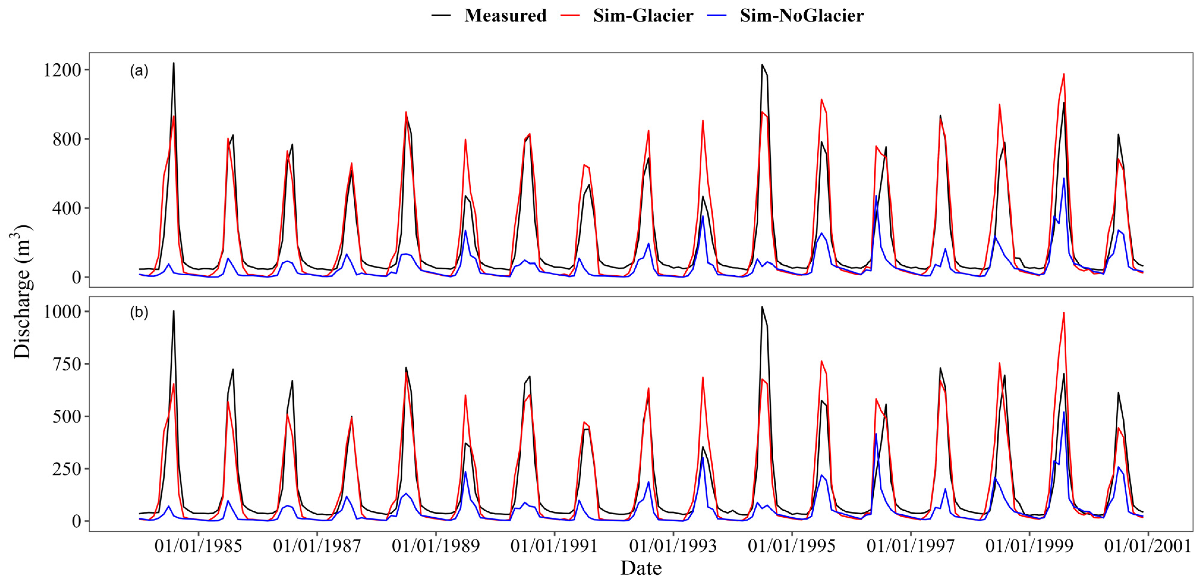
4.2. Model Calibration and Validation

All calibration parameter adjustments are included in a single file in SWAT+ to avoid changing them in their respective input files as SWAT does, which allows for much more rapid model adjustment, faster calibration, and better tracking of modified parameters. For calibration parameters, the desired change (e.g., new value, additive, or multiplicative change) and the spatial objects subject to the changes were specified. The model will automatically override all the corresponding values in the original data files based on the user-defined parameters in the calibration file.

Manual calibration of distributed watershed models like SWAT is proven to be difficult and almost infeasible in many large-scale applications in a previous study [27]. Instead of applying this labor-intensive way, automated calibration methods are often preferred. The autocalibration procedure described by prior research [63], known as the Integrated Parameter Estimation and Uncertainty Analysis Tool Plus (IPEAT+), which is an optimization and auto-calibration tool integrated with SWAT+ source code, was modified and incorporated into this extended model (SWAT+ Glacier) to implement auto calibration and validation. This algorithm provides an open-source and flexible auto-calibration workflow that can be incorporated with modified SWAT+ with minor efforts. Since various changes have been made to the original model, some adjustments must be made to allow IPEAT+ to adapt the new output file format and be able to read newly altered input files, which are mainly considered to be those parameter ranges involved with predicting glacier and snow processes correctly; the results indicated that it demonstrated a good performance in calibrating and validating the modified SWAT+ model.

Given the results from the sensitivity analysis above, the refreezing factor (gla_rf) is one of the most sensitive parameters to the runoff simulation since it directly determines the portion of the glacier meltwater that contributes to the main channel, while runoff in the UYR basin greatly relies on the contribution of glacier meltwater as previous studies indicated. Meanwhile, the value change could potentially result in the unreasonable value occurrence of both the temperature and solar radiation factor in glacier HRUs due to the high dependence among these mentioned parameters and lack of supporting observation data. Under this consideration, some parameters that are not highly sensitive to the simulation results and those with high sensitivity that could be a potential obstacle to other parameters are excluded in the calibration procedure. For example, a fixed empirical value of 0.2 was taken for the glacier refreezing factor (gla_rf) in this paper as former research [33,64] suggested. As Figure 4 presented, similar calibration results can be achieved in a much more effective way with only a few of the most sensitive parameters instead of all related parameters considered. Specifically, the top five sensitive parameters (glacier temperature factor and maximum/minimum sublimation coefficient of snow/glacier) introduced above were applied to the calibration and validation period. The value of those modified parameters can be found in

Table 2. Values of parameters related to glacier and snow processes.

Parameters	Description	Unit	Default Value	Calibrated Value
sno_sblfmx	Snow sublimation factor on 21 June	none	0.6	0.86
sno_sblfmn	Snow sublimation factor on 21 December	none	0.2	0.12
gla_tf	Temperature factor of glacier	mm °C−1 h−1	0.05	0.02
gla_sblfmx	Glacier sublimation factor on 21 June	none	0.8	0.83
gla_sblfmn	Glacier sublimation factor on 21 December	none	0.2	0.19
snofall_tmp	Snowfall temperature	degrees	0	-
snomelt_tmp	Snow melt base temperature	degrees	0	-
snomelt_max	Snow melt degree-day factor on 21 June	mm °C−1 day−1	0	-
snomelt_min	Snow melt degree-day factor on 21 December	mm °C−1 day−1	0	-
snomelt_lag	Snowpack temperature lag factor	none	0	-
firn_alpha	The basal turnover rate of snow to ice	mm	0.003	-
fresh_albedo	Fresh snow albedo while 1 °C.	none	0.8	-
const	Coefficient to calculate snow albedo	none	0.05	-
glamelt_tmp	Glacier melt base temperature	degrees	1	-
gla_srf	Solar radiation factor of glacier	m2 mm W−1 h−1	0.0094	-
gla_rf	Refreezing portion of glacier melt	none	0.2	-
gla_m	Coefficient m in V-A relationship	none	1.35	-
gla_n	Coefficient n in V-A relationship	none	0.5	-
gla_albedo	Glacier albedo	none	0.8	-

.

Despite a single objective function being minimized to seek a better fit between observation data and simulation outputs during the optimization procedure, all five statistics (NSE, R², PBIAS, MSE, RMSE) built into IPEAT+ will be calculated and stored in the output file. Since the correlation coefficient (R²) is good enough before calibration (0.81 and 0.79 for Kaqun and Kuluklangan, respectively), a transformed form of NSE known as OF, described in the following expression, is used for the optimization.

$$\mathrm{OF}={\displaystyle \sum }_{m=1}^M\left(1-NS{E}_m\right)$$

(6)

where OF is the transformed objective function; $NS{E}_m$ is the NSE value of aggregated modeling responses m; and M is the total number of modeling responses (in this study, M = 1500 for streamflow). Note that the best potential value of OF is zero if all $NS{E}_m$ are equal to one.

Since there are no measured glacier and snow data available, the monthly measured discharge data series from the two hydrological stations above were split into two segments from 1984 to 2000 and from 2001 to 2015 to calibrate and validate the SWAT+ Glacier model, respectively. As depicted in Figure 5, the simulated monthly discharge with the glacier module has been significantly improved even before calibration, especially in summer while it is undervalued in winter. Specifically, as Figure 6 illustrated, in comparison with the original model, the performance of the model incorporated with the glacier module has been greatly improved, since the average value of R² enhanced from 0.32 to 0.84 and NSE from 0.29 to 0.83, respectively.

As illustrated in Figure 7, the correlation coefficient (R²) between the monthly observed and simulated discharge rate under calibration period from 1984 to 2000 is 0.86 and 0.82 for two hydrological stations, with an average value of 0.84. The NSE for monthly discharge rate is 0.85 and 0.81, with an average of 0.83 under the calibration period. Even if slight underestimation remains in the validation period, the value from both hydrological stations in winter has been greatly improved, especially in the early validation period. The results overall present a well-simulated output of streamflow processes in the data-scarce glacierized area with the coupled SWAT+ model with the described glacier module and demonstrated that the introduced calibration algorithm is a low-cost, easily applied, and effective method for parameter optimization.

4.3. Temporal Variations of Glacier Runoff

The multi-year monthly averaged runoff, as well as the glacier contributions of the study area from 1984 to 2015, are conducted and plotted in Figure 8 below. We can infer that the glacier contribution to the total runoff in the study area ranges from 0.1% (December) to 67.5% (September) while glacier runoff is intensively distributed in the summer season (June to August), accounting for about 78.5% of the total glacier runoff generated in the current year. Glacier runoff decreased after September and maintained a negligible amount of 1.1 × 10⁶ m³ (2.1% of the annual glacier runoff) during the whole winter season due to the negative air temperature, and gradually increased until March of the next year.

According to the comparison of the observed and simulated discharge of the two hydrological stations at the seasonal level (Figure 9), the coefficient of determination (R²) suggested satisfactory performances in summer and autumn, while clarity underestimation results occurred in winter and spring, and an especially bad result occurred in winter for Kaqun station.

5. Discussion

Notably, SWAT+ is still under development, although a lot of new features have been added, some algorithms are not completely incorporated into the source code compared to the SWAT model. For instance, previous research [33,35] has confirmed that the inclusion of elevation bands could result in a better fit with the measured discharge rate, while this is still lacking in the current version. The application of elevation bands reconstructs the spatial distribution of temperature and precipitation at the vertical direction, which leads to a more realistic depiction of hydrological-related processes. The characteristic of the overestimation of discharge rate in the summer season denoted in Figure 7 might be linked to the lack of the participation of elevation bands, which indicates that the integration and expansion of some good features such as the elevation bands algorithm in future work could be helpful to reduce simulation uncertainty and improve model performance to some extent.

Finding appropriate parameter sets is both vital for model performance evaluation and also a problem, due to the lack of good quality and long-term observed glacier data in remote glacierized catchments. Good or even satisfactory simulation results in the glacierized area might not be able to represent unambiguous parameter sets since glaciers are often assumed to be unlimited sources or storages of water. For this reason, except for some measures, such as constraining the range of related parameters or multiple processes, criteria calibration should be implemented, and available measured glacier data such as area, mass balance, glacial equilibrium lines, albedo, volume, storage, and thickness, especially over long periods, should be collected to reduce modeling uncertainty.

Glacier hydrological processes, such as glacier flow, debris cover, etc., are not completely considered in this study. Additionally, the processes coupled in this model are based on the experienced coefficients and formulas, these parameters are relatively weak in verification due to the non-availability of field data. However, this work still provides new understanding for further study on fieldwork, theoretical representation, and parameterization of these terms within a watershed hydrological model.

On the other hand, the uncertainties of the input data also have a great influence on the modeling results, especially for temperature and precipitation data, which are often scarce in glacierized watersheds due to the high altitudes, complex terrain conditions, and difficult accessibilities. Glacier meltwater greatly relies on temperature, especially the temperature-index methods that take air temperature as the index and the energy budget of glacier mass balance. Overestimated temperature and underestimated glacier melt temperature may cause more meltwater, and the reverse held as well. The temperature index that divides precipitation into rainfall and snowfall also influences the uncertainty of the results, a lower index provides less liquid precipitation, and consequently more contribution to streamflow from glacier and snow. As reported in previous research [65], the uncertainties of the gridded climate products primarily originate from the errors of models and observations in the data assimilation system. Therefore, more intensive ground observations and more accurate reanalysis data, especially precipitation data, are needed in future research [66,67].

Nevertheless, the presented SWAT+ Glacier model provides a complete workflow from modeling to calibration and validation using remote sensing data in the data-scarce glacierized catchment. Our enhanced model has a great potential in quantitively analyzing the contribution of hydrological components to climate change, specifically the effects of the glacier and snow cover change on streamflow in highly glacierized watersheds. In the meantime, the employed degree-day algorithm is proven to be a simple and feasible way of simulating glacier meltwater in the watershed scale, with further understanding of glacier and snow processes, and other more complex approaches such as energy mass balance, glacier dynamics, and debris cover may be considered in subsequent research.

6. Conclusions

In this study, an extended degree-day glacier melt algorithm considering radiation effect, dynamic hydrological units, as well as multi-source remote sensing data, were combined and coupled with the SWAT+ model to simulate glacier melt contribution to streamflow and evaluate glacier change in data scarce watersheds. The sensitivity analysis revealed that the most sensitive parameters in the study area are related to snow and glacier hydrological processes, which are the maximum/minimum glacier/snow sublimation factor (gla/sno_sblfmx/mn), temperature factor of the glacier (gla_tmp_factor), and refreezing factor of the glacier (gla_rf), given the high reliance on the runoff to glacier meltwater in this region. Additionally, IPEAT+ was also modified and incorporated into the model for calibration and validation using the detected sensitive parameter set. In general, despite the uncertainty of the glacier extent estimation, vertical distribution of climate variables, as well as the systematic errors of the model, including the glacier process and remote sensing data have significantly improved model performance on the basin scale. This implies that model calibration using monthly discharge data is also a feasible option in data-scarce and glacier-meltwater-dominated catchments.

References

1. IPCC. IPCC Special Report on the Ocean and Cryosphere in a Changing Climate; Cambridge University Press: Cambridge, UK; New York, NY, USA, 2019; pp. 3–35. [CrossRef]
2. Kang, S.; Guo, W.; Zhong, X.; Xu, M. Changes in the Mountain Cryosphere and Their Impacts and Adaptation Measures. Clim. Chang. Res. 2020, 16, 143–152. [Google Scholar] [CrossRef]
3. Zhang, Q.; Chen, Y.; Li, Z.; Fang, G.; Xiang, Y.; Li, Y.; Ji, H. Recent Changes in Water Discharge in Snow and Glacier Melt-Dominated Rivers in the Tienshan Mountains, Central Asia. Remote Sens. 2020, 12, 2704. [Google Scholar] [CrossRef]
4. Chordia, J.; Panikkar, U.R.; Srivastav, R.; Shaik, R.U. Uncertainties in Prediction of Streamflows Using SWAT Model—Role of Remote Sensing and Precipitation Sources. Remote Sens. 2022, 14, 5385. [Google Scholar] [CrossRef]
5. Yang, J.; Huang, M.; Zhai, P. Performance of the CRA-40/Land, CMFD, and ERA-Interim Datasets in Reflecting Changes in Surface Air Temperature over the Tibetan Plateau. J. Meteorol. Res. 2021, 35, 663–672. [Google Scholar] [CrossRef]
6. Jiang, Q.; Li, W.; Fan, Z.; He, X.; Sun, W.; Chen, S.; Wen, J.; Gao, J.; Wang, J. Evaluation of the ERA5 Reanalysis Precipitation Dataset over Chinese Mainland. J. Hydrol. 2021, 595, 125660. [Google Scholar] [CrossRef]
7. He, X.; Pan, M.; Wei, Z.; Wood, E.F.; Sheffield, J. A Global Drought and Flood Catalogue from 1950 to 2016. Bull. Am. Meteorol. Soc. 2020, 101, E508–E535. [Google Scholar] [CrossRef] [Green Version]
8. Sharma, A.; Wasko, C.; Lettenmaier, D.P. If Precipitation Extremes Are Increasing, Why Aren’t Floods? Water Resour. Res. 2018, 54, 8545–8551. [Google Scholar] [CrossRef]
9. Bolch, T.; Kulkarni, A.; Kääb, A.; Huggel, C.; Paul, F.; Cogley, J.; Frey, H.; Kargel, J.; Fujita, K.; Scheel, M.; et al. The State and Fate of Himalayan Glaciers. Science 2012, 336, 310–314. [Google Scholar] [CrossRef] [Green Version]
10. Rounce, D.R.; Hock, R.; Shean, D.E. Glacier Mass Change in High Mountain Asia Through 2100 Using the Open-Source Python Glacier Evolution Model (PyGEM). Front. Earth Sci. 2020, 7, 331. [Google Scholar] [CrossRef]
11. Zhang, H.; Li, Z.; Zhou, P. Mass Balance Reconstruction for Shiyi Glacier in the Qilian Mountains, Northeastern Tibetan Plateau, and Its Climatic Drivers. Clim. Dyn. 2021, 56, 969–984. [Google Scholar] [CrossRef]
12. Zhang, S.; Gao, X.; Zhang, X.; Hagemann, S. Projection of Glacier Runoff in Yarkant River Basin and Beida River Basin, Western China. Hydrol. Proc. 2012, 26, 2773–2781. [Google Scholar] [CrossRef]
13. Zhang, Y.; Enomoto, H.; Ohata, T.; Kitabata, H.; Kadota, T.; Hirabayashi, Y. Projections of Glacier Change in the Altai Mountains under Twenty-First Century Climate Scenarios. Clim. Dyn. 2016, 47, 2935–2953. [Google Scholar] [CrossRef]
14. Guo, X.; Pomeroy, J.W.; Fang, X.; Lowe, S.; Li, Z.; Westbrook, C.; Minke, A. Effects of Classification Approaches on CRHM Model Performance. Remote Sens. Lett. 2012, 3, 39–47. [Google Scholar] [CrossRef]
15. Zhao, Q.; Ye, B.; Ding, Y.; Zhang, S.; Shangguan, D.; Zhao, C.; Wang, J.; Wang, Z. Hydrological Process of a Typical Catchment in Cold Region: Simulation and Analysis. J. Glaciol. Geocryol. 2011, 33, 595–605. [Google Scholar]
16. Wortmann, M.; Bolch, T.; Su, B.; Krysanova, V. An Efficient Representation of Glacier Dynamics in a Semi-Distributed Hydrological Model to Bridge Glacier and River Catchment Scales. J. Hydrol. 2019, 573, 136–152. [Google Scholar] [CrossRef] [Green Version]
17. Bergström, S. Development and Application of a Conceptual Runoff Model for Scandinavian Catchments; Sveriges Meteorologiska och Hydrologiska Institut: Norrköping, Switzerland, 1976; p. 134.
18. Ahmad, B.; Usman, M.; Syed, A.; Haider, S. Contribution of Glacier, Snow and Rain Components in Flow Regime Projected with HBV Under AR5 Based Climate Change Scenarios Over Chitral River Basin (Hindukush Ranges, Pakistan). Int. J. Clim. Res. 2020, 4, 24–36. [Google Scholar] [CrossRef]
19. Gao, H.; He, X.; Ye, B.; Gao, X. The Simulation of HBV Hydrology Model in the Dongkemadi River Basin, Headwater of the Yangtze River Full-Text in Chinese. J. Glaciol. Geocryol. 2011, 33, 171–181. [Google Scholar]
20. Hagg, W.; Nesgaard, T. Modelling of Hydrological Response to Climate Scenarios in Glacierised Central Asian Catchments. Geophys. Res. Abstr. 2005, 7, 06192. [Google Scholar]
21. Kaser, G.; Grosshauser, M.; Marzeion, B. Contribution Potential of Glaciers to Water Availability in Different Climate Regimes. Proc. Natl. Acad. Sci. USA 2010, 107, 20223–20227. [Google Scholar] [CrossRef] [Green Version]
22. Zhou, P.; Zhang, H.; Li, Z. Impact of Climate Change on the Glacier and Runoff of a Glacierized Basin in Harlik Mountain, Eastern Tianshan Mountains. Remote Sens. 2022, 14, 3497. [Google Scholar] [CrossRef]
23. Omani, N.; Srinivasan, R.; Smith, P.K.; Karthikeyan, R. Glacier Mass Balance Simulation Using SWAT Distributed Snow Algorithm. Hydrol. Sci. J. 2017, 62, 546–560. [Google Scholar] [CrossRef]
24. Hock, R. Glacier Melt: A Review of Processes and Their Modelling. Prog. Phys. Geogr. Earth Environ. 2005, 29, 362–391. [Google Scholar] [CrossRef]
25. Omani, N.; Srinivasan, R.; Karthikeyan, R.; Smith, P. Hydrological Modeling of Highly Glacierized Basins (Andes, Alps, and Central Asia). Water 2017, 9, 111. [Google Scholar] [CrossRef] [Green Version]
26. Liu, J.; Long, A.; Deng, X.; Yin, Z.; Deng, M.; An, Q.; Gu, X.; Li, S.; Liu, G. The Impact of Climate Change on Hydrological Processes of the Glacierized Watershed and Projections. Remote Sens. 2022, 14, 1314. [Google Scholar] [CrossRef]
27. Arnold, J.G.; Moriasi, D.N.; Gassman, P.W.; Abbaspour, K.C.; White, M.J.; Srinivasan, R.; Santhi, C.; Harmel, R.D.; van Griensven, A.; Liew, M.W.V.; et al. SWAT: Model Use, Calibration, and Validation. Trans. ASABE 2012, 55, 1491–1508. [Google Scholar] [CrossRef]
28. Gassman, P.W.; Reyes, M.R.; Green, C.H.; Arnold, J.G. The Soil and Water Assessment Tool: Historical Development, Applications, and Future Research Directions. Trans. ASABE 2007, 50, 1211–1250. [Google Scholar] [CrossRef] [Green Version]
29. Tan, M.L.; Gassman, P.W.; Srinivasan, R.; Arnold, J.G.; Yang, X. A Review of SWAT Studies in Southeast Asia: Applications, Challenges and Future Directions. Water 2019, 11, 914. [Google Scholar] [CrossRef] [Green Version]
30. Tan, M.L.; Gassman, P.W.; Yang, X.; Haywood, J. A Review of SWAT Applications, Performance and Future Needs for Simulation of Hydro-Climatic Extremes. Adv. Water Resour. 2020, 143, 103662. [Google Scholar] [CrossRef]
31. Schaefli, B.; Hingray, B.; Niggli, M.; Musy, A. A Conceptual Glacio-Hydrological Model for High Mountainous Catchments. Hydrol. Earth Syst. Sci. 2005, 9, 95–109. [Google Scholar] [CrossRef] [Green Version]
32. Huang, S.; Krysanova, V.; Hattermann, F.F. Projection of Low Flow Conditions in Germany under Climate Change by Combining Three RCMs and a Regional Hydrological Model. Acta Geophys. 2013, 61, 151–193. [Google Scholar] [CrossRef]
33. Luo, Y.; Arnold, J.; Liu, S.; Wang, X.; Chen, X. Inclusion of Glacier Processes for Distributed Hydrological Modeling at Basin Scale with Application to a Watershed in Tianshan Mountains, Northwest China. J. Hydrol. 2013, 477, 72–85. [Google Scholar] [CrossRef]
34. Ji, H.; Fang, G.; Yang, J.; Yaning, C. Multi-Objective Calibration of a Distributed Hydrological Model in a Highly Glacierized Watershed in Central Asia. Water 2019, 11, 554. [Google Scholar] [CrossRef]
35. Yin, Z.; Feng, Q.; Liu, S.; Zou, S.; Li, J.; Yang, L.; Deo, R. The Spatial and Temporal Contribution of Glacier Runoff to Watershed Discharge in the Yarkant River Basin, Northwest China. Water 2017, 9, 159. [Google Scholar] [CrossRef] [Green Version]
36. Pellicciotti, F.; Brock, B.; Strasser, U.; Burlando, P.; Funk, M.; Corripio, J. An Enhanced Temperature-Index Glacier Melt Model Including the Shortwave Radiation Balance: Development and Testing for Haut Glacier d’Arolla, Switzerland. J. Glaciol. 2005, 51, 573–587. [Google Scholar] [CrossRef]
37. Bieger, K.; Arnold, J.G.; Rathjens, H.; White, M.J.; Bosch, D.D.; Allen, P.M.; Volk, M.; Srinivasan, R. Introduction to SWAT+, A Completely Restructured Version of the Soil and Water Assessment Tool. J. Am. Water Resour. Assoc. 2017, 53, 115–130. [Google Scholar] [CrossRef]
38. Liu, S.; Yao, X.; Guo, W.; Xu, J.; Shangguan, D.; Wei, J.; Bao, W.; Wu, L. The Contemporary Glaciers in China Based on the Second Chinese Glacier Inventory. Acta Geogr. Sin. 2015, 70, 3–16. [Google Scholar] [CrossRef]
39. Liu, S.; Guo, W.; Xu, J. The Second Glacial Catalogue Data Set of China (v1.0). Natl. Glacial Frozen Desert Sci. Data Cent. 2019. [Google Scholar] [CrossRef]
40. Neitsch, S.L.; Arnold, J.G.; Kiniry, J.R.; Williams, J.R. Soil and Water Assessment Tool Theoretical Documentation, Version 2009; Texas Water Resources Institute: College Station, TX, USA, 2001.
41. Zhao, Q.; Ye, B.; Ding, Y.; Zhang, S.; Yi, S.; Wang, J.; Shangguan, D.; Zhao, C.; Han, H. Coupling a Glacier Melt Model to the Variable Infiltration Capacity (VIC) Model for Hydrological Modeling in North-Western China. Environ. Earth Sci. 2013, 68, 87–101. [Google Scholar] [CrossRef]
42. Brock, B.W.; Willis, I.C.; Sharp, M.J. Measurement and Parameterization of Albedo Variations at Haut Glacier d’Arolla, Switzerland. J. Glaciol. 2000, 46, 675–688. [Google Scholar] [CrossRef] [Green Version]
43. Chen, Y.; Hu, L.; Yan, W.; Zhang, M.; Liu, J.; De, J. Study of the Changes in Summer Climate and Runoff in Two Upper Streams of the Yarkant River. J. Glaciol. Geocryol. 2014, 36, 678–684. [Google Scholar]
44. Huang, S.; Krysanova, V.; Zhai, J.; Su, B. Impact of Intensive Irrigation Activities on River Discharge Under Agricultural Scenarios in the Semi-Arid Aksu River Basin, Northwest China. Water Resour. Manag. 2015, 29, 945–959. [Google Scholar] [CrossRef]
45. Yi, Y.; Liu, S.; Zhu, Y.; Wu, K. Spatiotemporal Variation of Snow Cover in the Yarkant River Basin during 2002–2018. Arid Land Geogr. 2021, 44, 15–26. [Google Scholar]
46. Li, J.; Qian, K.; Liu, Y.; Yan, W.; Yang, X.; Luo, G.; Ma, X. LSTM-Based Model for Predicting Inland River Runoff in Arid Region: A Case Study on Yarkant River, Northwest China. Water 2022, 14, 1745. [Google Scholar] [CrossRef]
47. Gao, X.; Ye, B.; Zhang, S.; Qiao, C.; Zhang, X. Glacier Runoff Variation and Its Influence on River Runoff during 1961–2006 in the Tarim River Basin, China. Sci. China Earth Sci. 2010, 53, 880–891. [Google Scholar] [CrossRef]
48. Gao, X.; Zhang, S.; Ye, B. Glacier Runoff Change in the Upper Stream of Yarkant River and Its Impact on River Runoff during 1961–2006. J. Glaciol. Geocryol. 2010, 32, 445–453. [Google Scholar]
49. Feng, T.; Liu, S.; Xu, J.; Guo, W.; Wei, J.; Zhang, Z. Glacier Change of the Yarkant River Basin from 1968 to 2009 Derived from the First and Second Glacier Inventories of China. J. Glaciol. Geocryol. 2015, 37, 1–13. [Google Scholar] [CrossRef]
50. Chen, Y.; Xu, X.; Hao, X.; Li, W.; Chen, Y.; Zhu, C.; Ye, Z. Fifty-Year Climate Change and Its Effect on Annual Runoff in the Tarim River Basin, China. Quat. Int. 2009, 208, 53–61. [Google Scholar] [CrossRef]
51. He, J.; Yang, K.; Tang, W.; Lu, H.; Qin, J.; Chen, Y.; Li, X. The First High-Resolution Meteorological Forcing Dataset for Land Process Studies over China. Sci. Data 2020, 7, 25. [Google Scholar] [CrossRef] [Green Version]
52. Yang, K.; He, J.; Tang, W.; Qin, J.; Cheng, C.C.K. On Downward Shortwave and Longwave Radiations over High Altitude Regions: Observation and Modeling in the Tibetan Plateau. Agric. For. Meteorol. 2010, 150, 38–46. [Google Scholar] [CrossRef]
53. Yang, K.; He, J. China Meteorological Forcing Dataset (1979–2018). Natl. Tibet. Plateau Data Cent. 2019. [Google Scholar] [CrossRef]
54. Wang, Y.; Chen, H.; Nan, Z.; Shang, Z. Modelling Permafrost Characteristics and Its Relationship with Environmental Constraints in the Gaize Area, Qinghai-Tibet Plateau, China. Remote Sens. 2022, 14, 5610. [Google Scholar] [CrossRef]
55. Jin, H.; Chen, X.; Zhong, R.; Pan, Y.; Zhao, T.; Liu, Z.; Tu, X. Corrected GCM Data through CMFD Data to Analysis Future Runoff Changes in the Source Region of the Yangtze River, China. Environ. Earth Sci. 2022, 81, 527. [Google Scholar] [CrossRef]
56. Zhang, G.; Nan, Z.; Yin, Z.; Zhao, L. Isolating the Contributions of Seasonal Climate Warming to Permafrost Thermal Responses Over the Qinghai-Tibet Plateau. J. Geophys. Res. Atmos. 2021, 126, e2021JD035218. [Google Scholar] [CrossRef]
57. Zhang, L.; Gao, L.; Chen, J.; Zhao, L.; Zhao, J.; Qiao, Y.; Shi, J. Comprehensive Evaluation of Mainstream Gridded Precipitation Datasets in the Cold Season across the Tibetan Plateau. J. Hydrol. Reg. Stud. 2022, 43, 101186. [Google Scholar] [CrossRef]
58. Sheng, Y. Monthly Runoff Data of Yeerqiang River Basin in Recent 60 Years. Natl. Glacial Frozen Desert Sci. Data Cent. 2019. [CrossRef]
59. Schuerz, C. SWATplusR: Running SWAT2012 and SWAT+ Projects in R. 2019. [Google Scholar] [CrossRef]
60. Nash, J.E.; Sutcliffe, J. River Flow Forecasting Through Conceptual Models: Part 1—A Discussion of Principles. J. Hydrol. 1970, 10, 282. [Google Scholar] [CrossRef]
61. Abbaspour, K.C.; Rouholahnejad, E.; Vaghefi, S.; Srinivasan, R.; Yang, H.; Kløve, B. A Continental-Scale Hydrology and Water Quality Model for Europe: Calibration and Uncertainty of a High-Resolution Large-Scale SWAT Model. J. Hydrol. 2015, 524, 733–752. [Google Scholar] [CrossRef] [Green Version]
62. Fang, G.; Yang, J.; Chen, Y.; Li, Z.; Ji, H.; Maeyer, P.D. How Hydrologic Processes Differ Spatially in a Large Basin: Multisite and Multiobjective Modeling in the Tarim River Basin. J. Geophys. Res. Atmos. 2018, 123, 7098–7113. [Google Scholar] [CrossRef]
63. Yen, H.; Park, S.; Arnold, J.G.; Srinivasan, R.; Chawanda, C.J.; Wang, R.; Feng, Q.; Wu, J.; Miao, C.; Bieger, K.; et al. IPEAT+: A Built-In Optimization and Automatic Calibration Tool of SWAT+. Water 2019, 11, 1681. [Google Scholar] [CrossRef] [Green Version]
64. Jiang, X.; Wang, N.; He, J.; Wu, X.; Song, G. A Distributed Surface Energy and Mass Balance Model and Its Application to a Mountain Glacier in China. Chin. Sci. Bull. 2010, 55, 2079–2087. [Google Scholar] [CrossRef]
65. Nie, S.; Luo, Y.; Wu, T.; Shi, X.; Wang, Z. A Merging Scheme for Constructing Daily Precipitation Analyses Based on Objective Bias-correction and Error Estimation Techniques. J. Geophys. Res. Atmos. 2015, 120, 8671–8692. [Google Scholar] [CrossRef] [Green Version]
66. Huang, Q.; Long, D.; Han, Z.; Han, P. High-Resolution Satellite Images Combined with Hydrological Modeling Derive River Discharge for Headwaters: A Step toward Discharge Estimation in Ungauged Basins. Remote Sens. Environ. 2022, 23, 286–300. [Google Scholar] [CrossRef]
67. Fan, M.; Xu, J.; Li, D.; Chen, Y. Response of Precipitation in Tianshan to Global Climate Change Based on the Berkeley Earth and ERA5 Reanalysis Products. Remote Sens. 2022, 14, 519. [Google Scholar] [CrossRef]
Figure 1. Framework of incorporating glacier hydrological process into SWAT+, where iyr stands for the number of the years (nyr in total); ida presents the number of the days (nda in total); isub is the subbasin number (msub in total); ihru is the hru number (mhru in total).
Remotesensing 14 06080 g001
Figure 2. Input data and location of the Upper Yarkant River (UYR) basin, (a) SRTM and hydrological stations, (b) Land use, (c) Soils, (d) Location of the UYR basin.
Remotesensing 14 06080 g002
Figure 3. Parameter sensitivity scores in the UYR basin using Sobol method.
Remotesensing 14 06080 g003
Figure 4. NSE value change during the first 150 calibration runs, the red solid line indicates the value change calibrated with all 25 parameters except for the glacier refreezing coefficient, while the green line describes the results computed with only the two most sensitive parameters using the Sobol method.
Remotesensing 14 06080 g004
Figure 5. Comparison of simulated and measured monthly discharge rate before calibration (1984–2015), (a) Kaqun station, (b) Kuluklangan station.
Remotesensing 14 06080 g005
Figure 6. Comparison of discharge simulated by SWAT+ and SWAT+Glacier; (a) Kaqun station, (b) Kuluklangan station.
Remotesensing 14 06080 g006
Figure 7. Comparison of simulated and measured monthly discharge rate after calibration and validation (1984–2015) in which calibration period ranged from 1984 to 2000 (light grey background), validated period ranged from 2001–2015; (a) Kaqun station, (b) Kuluklangan station.
Remotesensing 14 06080 g007
Figure 8. Simulated total runoff and glacier runoff contributions on the multi-year monthly level in the UYR basin.
Remotesensing 14 06080 g008
Figure 9. Model performance at seasonal statistics of the two hydrological stations from 1984 to 2015.
Remotesensing 14 06080 g009