Abstract
Projections of future climate are sensitive to the representation of upper-ocean diurnal variability, including the diurnal cycle of winds. Two different methods suitable for time series with missing data are used here to characterize how observed diurnal winds vary over the year. One is based on diurnal composites of mooring data, and the other is based on harmonic analysis via a least squares fit and is able to isolate annual (i.e., 1 cycle per year) modulation of diurnal variability. Results show that the diurnal amplitude in meridional winds is larger than in zonal winds and peaks in the tropical Pacific, where diurnal variability in zonal winds is overall weaker compared to other basins. Furthermore, the amplitude and phasing of diurnal winds in the tropical oceans are not uniform in time, with overall larger differences through the year in the meridional component of tropical winds. Estimating the annual modulation of the diurnal signal implies resolving both the diurnal energy peak and also the modulation of this peak by the annual cycle. This leads to a recommendation for sampling at least 6 times per day and for a duration of at least 3 years.
1. Introduction
Diurnal variability is one of the most persistent features of the Earth’s climate system. Diurnal variations in solar heating in the atmosphere and at the Earth’s surface contribute to the generation of internal gravity waves and other atmospheric motions that can lead to diurnal variations in surface winds [1,2,3,4,5]. Over the tropical ocean and island regions, diurnal and semi-diurnal variations in surface winds are attributed to a variety of mechanisms [5,6,7,8] including changes in local forcing such as solar heating of local topography, latent heating in moist convective regions, and differential solar heating over adjacent water and land surfaces. Because large-scale vertical motion in the lower atmosphere and upper ocean is associated with mean convergence/divergence of surface winds, diurnal variations in surface winds can modulate oceanic mixing [9] as well as atmospheric convection in the deep tropics [10,11].
The diurnal cycle in winds and sea surface temperature is modulated on intraseasonal timescales (e.g., by the Madden Julian Oscillation as described in [12,13]), as well as seasonal and interannual timescales (see, e.g., in [4,14,15]). Although the sun crosses the equator twice a year, there is a strong annual cycle in the Tropics, and changes in temperatures and pressure gradients with seasons can drive changes in surface winds on diurnal and longer timescales [4]. Previous research [4] shows that the amplitudes of diurnal meridional wind variations in the tropical Pacific are larger during the cold season (June–November) than the warm season (December–May), with similar spatial patterns in the two seasons. Seasonal and interannual cycles in winds and wind-driven mixing can in turn modulate diurnal warming in the upper ocean [16,17].
If winds were the only diurnally varying component of the climate system, we might hypothesize that maxima and minima within the diurnal cycle would cancel each other out to produce no net impact on the climate system. Yet, diurnal winds interact with diurnal surface buoyancy fluxes and diurnal sea surface temperatures and can drive local and nonlocal mixing and rectify due to nonlinear processes. Characterizing diurnal winds and how they change in different months of the year based on observations is the first step towards understanding these interactions and how they modulate diurnal variations in mixed-layer depth and turbulent mixing (see, e.g., in [9,18,19]). Quantifying annual modulation of diurnal winds is also important to cross-calibrate wind-measuring satellites that have different equator crossing times in order to create climate records. While mesoscale variability in the wind field will produce significant random spread in the differences between instruments, not accounting for the diurnal cycle will produce systematic errors that will remain after averaging [20]. For this reason, the Committee on Earth Observation Satellites (CEOS) has recommended that a minimum of three scatterometers be flown, with different equator crossings, and preferably with one satellite in a non-sun-synchronous orbit [21].
Most satellites that measure wind operate on sun-synchronous orbits, meaning that measurements are collected at two fixed local times, often 6 a.m. and 6 p.m. Sun synchronous orbits are well suited for determining representative large-scale wind patterns that vary on time scales longer than a few days. The twice-a-day sampling of a single satellite is at the Nyquist frequency of the diurnal cycle, meaning that no phase information and no precise amplitudes can be obtained, thus leaving an incomplete picture of diurnal winds [22]. The advent of scatterometry has brought a greatly expanded global perspective on diurnal wind variability. Scatterometer observations show that land-breeze/sea-breeze circulation patterns [5,22,23,24,25] are ubiquitous along coastlines across the globe, particularly in the summer [5,22,25,26]. Diurnal winds also extend across the tropics throughout the region equatorward of 30° latitude [2,5,15,22,25,26]. Much of the satellite-based analysis of diurnal winds has focused on day–night differences in QuikSCAT observations [22,27] or on observations from the six-month-long QuikSCAT/ADEOS-2 tandem mission in 2003 [5,25,26]. The short duration of the QuikSCAT/ADEOS-2 tandem mission and the limitations of the tandem mission temporal sampling have left open a number of questions about the detailed temporal structure of diurnal winds and about the variability of diurnal winds on seasonal to interannual time scales. Recently, Turk et al. [15] demonstrated a methodology to merge the speed-only measurements from passive microwave radiometers with the wind vector measurements available from scatterometers, allowing them to estimate the diurnal and semi-diurnal wind vector components during 2007–2017 and to compare El Niño versus La Niña conditions.
While satellite-based studies and buoy analyses (see, e.g., in [2,4,5,15,22,25,26]) have broadly characterized the spatial structure of diurnal variability, the limited temporal duration of records available for previous studies or (in some cases) the regional focus left open questions about the seasonal and interannual variations in diurnal variability [22].
Here, we address this gap by describing the diurnal variability in surface winds over the tropical ocean from buoy measurements, with a specific focus on how diurnal winds (zonal, meridional, and overall speed) vary in different months of the year due to annual (i.e., 1 cycle per year) modulation of the diurnal signal. We consider variations in both the amplitude of the diurnal cycle and its phase (e.g., hour of the diurnal peak). Our analysis provides an updated characterization of diurnal winds from mooring data: we use measurements for more years and locations compared to previous analysis (see, e.g., in [4,15]), and we develop a new method that allows us to extract more detailed information about the temporal variability. Our approach provides a framework to assess how satellite-like sampling scenarios (i.e., observations with limited temporal coverage) capture the diurnal signal of interest. The dataset and methodology are described in Section 2 and Section 3, respectively. Results from applying two different approaches to satellite-like pseudo-observations are presented in Section 4. The annual modulation of diurnal variability in the tropical ocean is described in Section 5. Summary and conclusions are given in Section 6.
2. Datasets
The Global Tropical Moored Buoy Array Program (GTMBA [28]) is a multi-national effort that provides real-time data for climate research and forecasting. Major components include the TAO/TRITON (Tropical Atmosphere Ocean [29]) array in the Pacific Ocean, PIRATA (Prediction and Research Moored Array in the Tropical Atlantic [30]) in the Atlantic, and RAMA (Research Moored Array for African-Asian-Australian Monsoon Analysis and Prediction [31]) in the Indian Ocean.
The moorings in the GTMBA are designed and built based primarily on the Autonomous Temperature Line Acquisition System (ATLAS [32]) moorings that were originally designed at the NOAA’s Pacific Marine Environmental Laboratory (PMEL) and on the Triangle Trans Ocean Buoy Network (TRITON) moorings designed by the Japan Agency for Marine-Earth Science and Technology (JAMSTEC). These moorings are specially designed to observe and measure the upper ocean and surface meteorological variables that drive air–sea interactions in the tropics. They are instrumented to provide long-term time series measurements of fine temporal resolution (minutes to hours) to resolve high-frequency fluctuations in the oceanic and surface atmospheric variables that would otherwise be aliased into the lower frequency climate signals. These moorings are fixed in location over the tropical ocean, and so the sampling is not variable in space or time (when the mooring is operational). Mooring data are made available by the GTMBA Project Office of NOAA/PMEL and allow better understanding of regional weather and climate variability on seasonal, interannual, and longer time scales, thus improving predictions of climate variations.
We take advantage of the high temporal resolution (10 min to a few hours depending on the site) of the GTMBA to characterize diurnal surface winds and to examine changes in these diurnal winds during different months of the year. We use records for which time periods of at least 3 years are available with gaps of 3 months or less and no more than 20% of data missing. While only eight sites have records with these characteristics in the Indian Ocean, the majority of sites in the Pacific and Atlantic Oceans meet these criteria (Figure 1), and some of the records employed in our analysis are longer than 6 years.
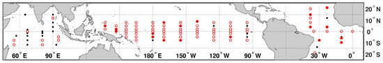
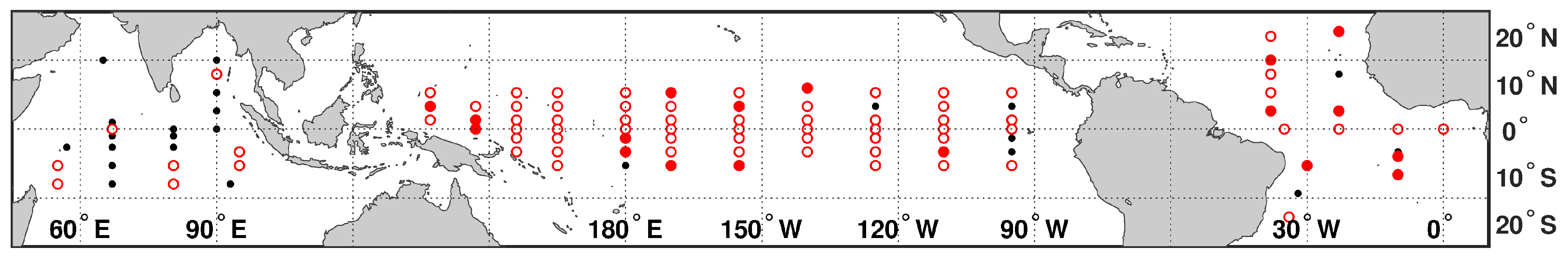
Figure 1.
Mooring sites. Moorings marked by red circles are selected for our analysis, i.e., records of at least 3 years are available with gaps of 3 months or less and no more than 1/5 of missing data. Filled red dots indicate moorings where at least 6 years of data are available. Black dots show the remaining mooring sites (not used here).
3. Methodology
Previous analyses of annual modulation of the diurnal cycle in surface winds (see, e.g., in [4,5,33]) have been based on binning the data in 1-h bins (separately for each month or season) and then fitting a diurnal cycle to the composite to estimate diurnal amplitude and phase for that month (or season). Results were compared with amplitude and phase for the full time series (i.e., from binning the data in 1-h bins for the full time series).
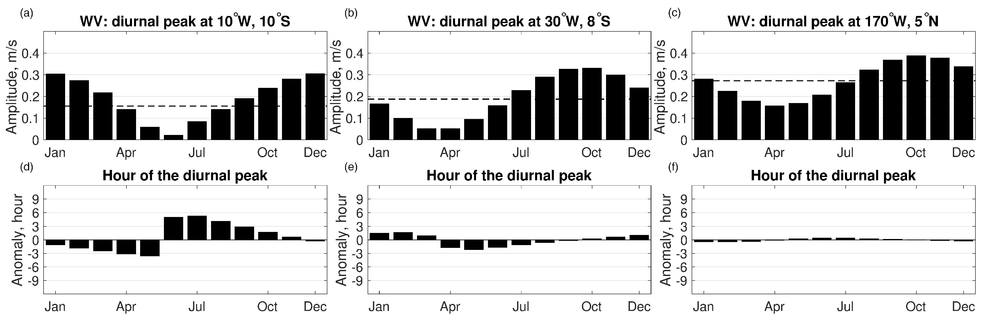
In this study, we compare estimates from this method with harmonic analysis designed to extract diurnal cycles and their annual modulation from the original time series. As described in Section 3.1 and Section 3.2, our harmonic analysis uses a least squares fit methodology, and thus this method can be used to derive the harmonic signals from irregular time series as well. The method allows for the inclusion of specific frequencies of interest, such as the diurnal frequency and the modulated components, as well as frequencies that can capture variability that we do not want to be aliased in the signal of interest. In doing so, the fit is able to isolate e.g., the annual (i.e., 1 cycle per year) modulation of diurnal winds, while composites for different months show seasonal modulation (e.g., the combination of annual and semi-annual modulation, if there is any semi-annual modulation and if it is resolved at all) and may include spurious signals. Compositing by month is also slightly affected by leap years which do not affect the least squares fit. Finally, the least squares fit methodology can take advantage of expected parameter magnitudes (e.g., less power in higher harmonics) for improved accuracy of the result. In the following analyses, the method based on binning the original mooring time series in 1-h bins and fitting a diurnal cycle to this composite will be referred to as CM (from “Composite”). The harmonic analysis will be referred to as LSF (from “Least Squares Fit”). Figure 2 shows examples of the results for LSF: depending on the location, the maximum and the annual mean diurnal amplitude during the year can be several times larger than the minimum (e.g., Figure 2a). Similarly, depending on the mooring location, we observe a change in the hour of the diurnal peak that varies from zero to several hours (e.g., Figure 2d–f).
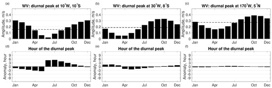
Figure 2.
Meridional wind (WV): examples of how (a–c) the amplitude and (d–f) the hour of the diurnal peak change during the year. In top panels (a–c), the black dashed line indicates the annual mean diurnal amplitude. In bottom panels (d–f), the vertical axes show the difference between the hour of the diurnal peak for each of the 12 months and the annual mean diurnal cycle. The location of the mooring where observations were measured is indicated in the title of the top panels.
3.1. LSF Method: Formulation
A single time series (), represented by an column vector of observations at a location (e.g., a buoy wind record), is described as a sum of harmonic components, i.e.,
In Equation (1),
- is the annual cycle and its five harmonics,
- are diurnal and semi-diurnal cycles,
- are modulations of the diurnal and semi-diurnal cycles,
- is a low-passed component,
- are the first two polynomial basis functions (a mean and a linear trend), and
- are residuals.
We write as an estimated time series plus residuals, i.e.,
with
The estimate of the model coefficients () for the different components is described in Section 3.2. Table 1 describes frequencies used to build , , , , thus the matrix in Equation (4). As an example, the matrix ( dimensions) contains the sine and cosine functions of the annual cycle and its five harmonics for a time series with N records:
with () and radians per day (rpd). Six seasonal harmonics correspond to one free parameter per month, and their use in the regression is similar to the monthly composite mean used by certain authors to identify and remove seasonality (see, e.g., in [34]), although the LSF can include prior expectations of lower amplitude in higher harmonics, which is harder to enforce with the compositing. includes frequencies and to estimate the annual modulation of the diurnal signal [35]. It also includes and for the semi-annual modulation [35]. includes frequencies starting at (Table 1) so as not to enforce periodicity: the interval between frequencies is equal to as resolving peaks in energy for frequencies in is not part of our goal. (The low-pass component and the mean and trend are included only to account for the red spectrum of wind variability in the fit.)

Table 1.
Frequencies (f, rpd) used to build , , , : minimum (), maximum (), and interval between frequencies (). includes components for modulation of the diurnal and semi-diurnal signal (rows labeled as part 1 and 2, respectively). Frequencies are defined as rpd (diurnal), rpd (annual), , , with the largest integer number of years less or equal to the length (L, in years) of the timeseries (L can be a non-integer).
Finally, is prepared with a time series of a mean and a linear trend:
where denotes a reference time, generally the center of the regression time window.
The time-independent basis function in Equation (7) is included in the regression to estimate a true time mean of the data. A simple time mean of the data is removed prior to regression. Because the data may be sampled irregularly within a finite time window, this simple time mean may contain a bias that needs to be adjusted with the mean computed from the regression.
3.2. LSF Method: Inverse Problem
From Equation (3), the model coefficients (see, e.g., in [36]) are
Assuming the amplitudes of the basis functions are uncorrelated, the model covariance matrix () is diagonal:
with the diagonals of , , , , and (i.e., expected variances at those frequencies) estimated as averages across all of the moorings. These estimates are computed from the discrete Fourier Transform of the wind data autocorrelation function (e.g., Figure 3), using the Wiener–Khinchin theorem [37].
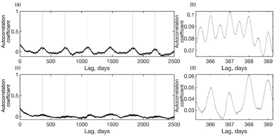
Figure 3.
Example of autocorrelation function (at 10°W, 10°S) showing annual, diurnal, and semi-diurnal oscillations in (a,b) zonal wind and (c,d) meridional wind. The right panel shows a portion of the left panel for time lags longer than a year, and the vertical gray lines in panels (a,c) mark years.
While applying this theorem is helpful to capture the shape of the power spectrum as averages across all of the moorings (to estimate the model covariance), it does not include phase and cannot provide accurate estimates of the details of the diurnal cycle for a finite record with missing data (not shown). Therefore, we designed the LSF method to estimate diurnal variability and annual modulation at individual mooring sites. Finally, the error covariance matrix () is assumed to be a scaled diagonal matrix,
meaning that the errors are uncorrelated between observations and have identical variances. In Equation (12), is the identity matrix and is a scalar (equal to 1 m/s) representing the expected level of homogeneous white noise in the data. Once model coefficients are estimated, we can compute variance and phase of the annual mean diurnal cycle (from , as this vector contains the amplitude of the fitted sine and cosine functions with diurnal frequency), and also identify how the diurnal cycle changes in different months of the year (using to reconstruct the modulated diurnal signal in the time domain to find the extrema).
4. Comparison of Methods
We first apply the CM and LSF methods to estimate the diurnal cycle and its annual modulation in a time series of surface wind observations from mooring data at 30°W, 8°S. At this site, semi-diurnal variability is larger than diurnal variability for the zonal wind (not shown). In contrast, diurnal variability is larger than semi-diurnal for the meridional wind. The meridional wind analysis shows that both the amplitude of the diurnal cycle and the time of the diurnal peak change during the year relative to annual mean values (Figure 2b,e). The minimum diurnal amplitude during the year is about a quarter of the annual mean diurnal amplitude and less than one-sixth the maximum diurnal amplitude in the year (Figure 2b). Overall, the diurnal amplitude is much larger in the second half of the year compared to the first half. The time of the diurnal peak changes by up to ∼4 h during the year, with more than 1-h differences between the diurnal peak in many of the individual months and the annual mean diurnal peak (Figure 2e). The late afternoon annual mean diurnal peak at this location and its variability through the seasons may represent open-ocean diurnal cycles driven by afternoon atmospheric boundary layer instabilities and their seasonal variations [2].
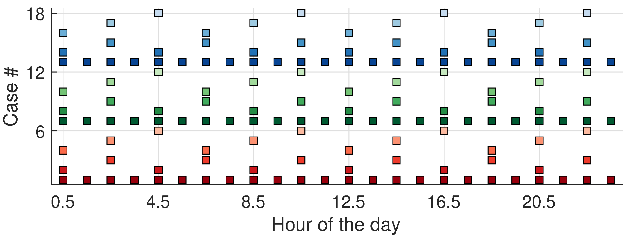
To evaluate the robustness of the CM and LSF results, we use the full time series at 30°W, 8°S, as well as different decimated versions of this time series, testing records of different lengths (up to 10 years), temporal resolutions (from 1 to 6 h time steps), and sampling times (i.e., hour of the day when samples are taken, as indicated for each case in Figure 4). Eighteen test cases are considered, subsampling the original 10-min wind record with coarser resolution scenarios designed to be representative of potential sampling by satellites (Figure 4). CM and LSF results are compared (for each method) across scenarios. For each method, results from different scenarios are compared to results from the 10-min original (full-length) record (i.e., the “best estimate” or “baseline” for each method). Our objectives are both to characterize how diurnal winds vary during the year and also to present a framework that can help identify satellite sampling requirements needed to capture both the diurnal variability and its annual modulation.
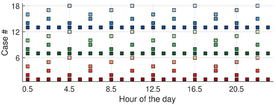
Figure 4.
Data distribution (by hour of the day) for test cases constructed from 10-min observations at 30°W, 8°S. The horizontal axis gives the time of day of the samples and the vertical axis is case number. Time series for different groups of cases are (red; case # 1 to 6) 10-year-, (green; 7 to 12) 5-year-, and (blue; 13 to 18) 3-year-long. For each record length, colors from darker to lighter indicate changes in sampling (e.g., data may be sparser in time and/or collected at different hours of the day). Case #1, 7, 13 are characterized by 1-h sampling. Case #2, 3, 8, 9, 14, 15 by 4-h sampling. Case #4 to 6, #10 to 12, #16 to 18 by 6-h sampling.
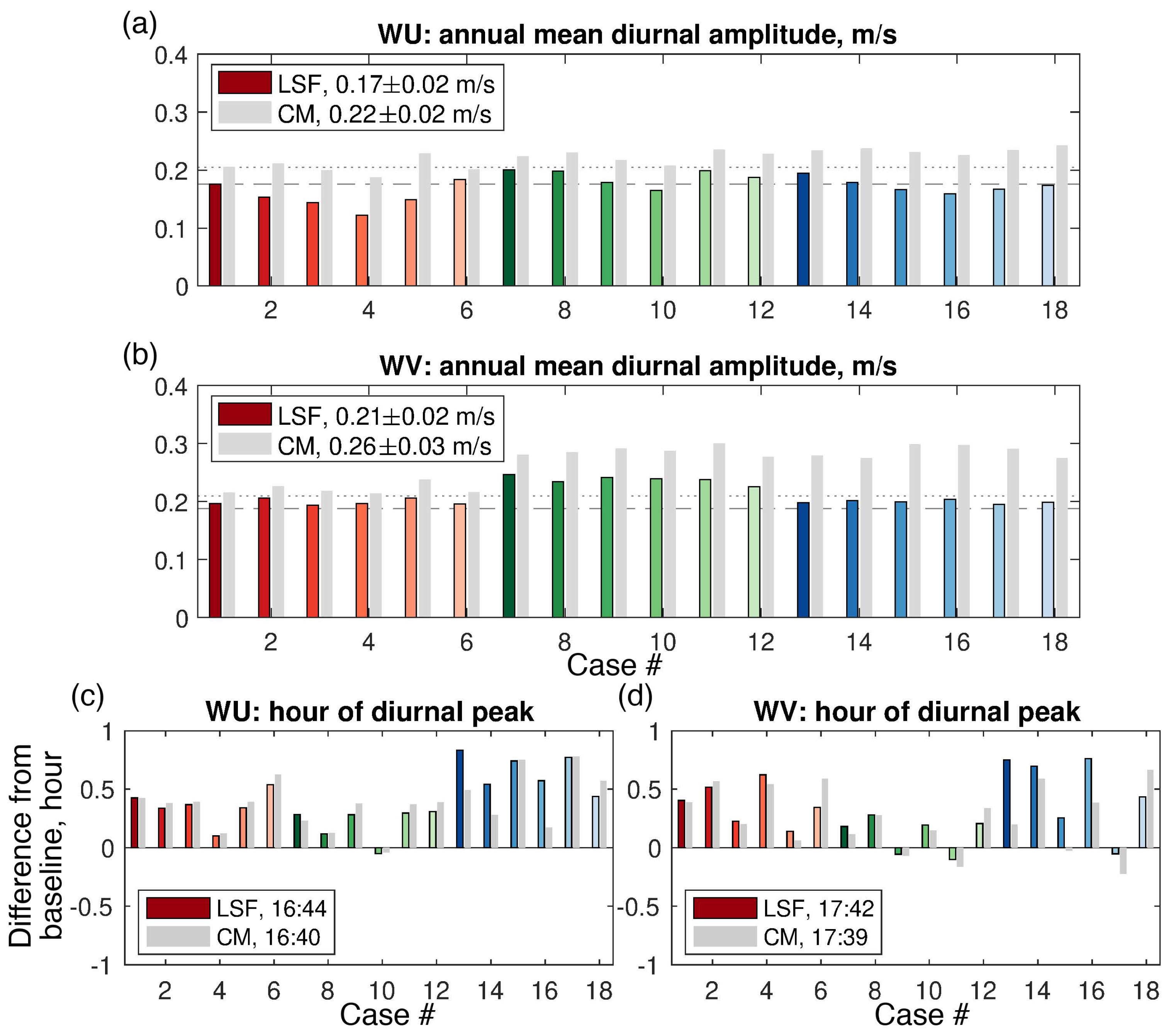
We start by analyzing amplitude and phase of the annual mean diurnal cycle in CM and LSF. For 3-year and 5-year time series, the CM method tends to overestimate the diurnal amplitude compared to the baseline 10-year record (e.g., gray bars compared to the dotted line in cases to in Figure 5a,b). The same is observed for the 5-year time series using LSF (e.g., green bars compared to the dashed line in Figure 5b). For 10-year time series (red bars), both methods provide a estimate of the annual mean diurnal amplitude that is close to the baseline, except for LSF in case for zonal wind (Figure 5a). The monthly 24-h composite of zonal wind at 30°W, 8°S shows semi-diurnal variability that varies interannually during the 10 years (not shown): this makes it difficult for LSF to capture details of the (smaller) diurnal variability in the signal, given the sparse 6-h sampling of case , the specific hours included in the sampling of case , and the phasing of the variability during the course of a day at this location. For the annual mean hour of the diurnal peak, different scenarios are consistent with one another and with the baseline for each method: in Figure 5c,d, all scenarios agree within less than 1 h, indicating that the data distribution does not affect the estimated hour of the day in either method.
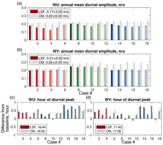
Figure 5.
Results for (a,c) zonal and (b,d) meridional surface wind at 30°W, 8°S, as sampled in Figure 4. Panels (a,b) show the annual mean diurnal peak from the (red, green, blue bars) LSF versus (gray bars) CM method. Panels (c,d) are for the hour of the annual mean diurnal peak: they show the differences between the estimates from decimated time series (using LSF versus CM method) and the baseline (i.e., corresponding estimates based on the longest and highest resolution data record). The more robust the method, the smaller the difference among results from different cases (as they are constructed by subsampling the same time series). In all panels, the horizontal axis is the case number and the bars for LSF are color coded by case number as in Figure 4. In panels (a,b), the legend indicates the average and standard deviation across scenarios for each method. In panels (c,d), the baseline estimates are indicated (as local time). In panels (b,d), the baseline estimates are indicated as gray lines: the line is dotted for the CM method, dashed for LSF.
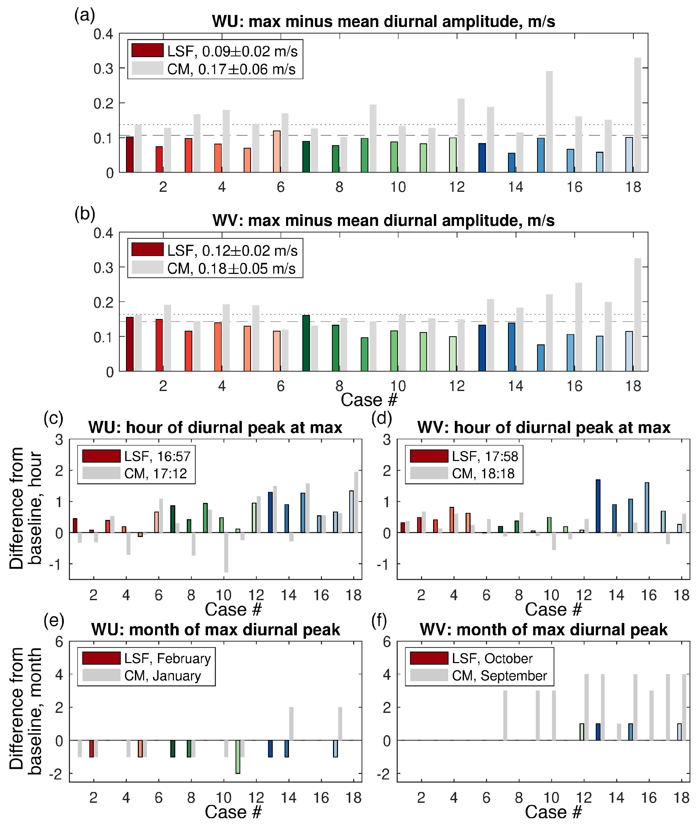
Next, we consider how the diurnal signal changes during the year. As described in Section 3, LSF can isolate the annual modulation, while results for CM are representative of the seasonal modulation. Both methods struggle to capture the difference between the maximum diurnal amplitude in the year and the annual mean diurnal amplitude for 3-year long timeseries of zonal wind: in Figure 6a (cases to ), bars for each method are often not close to the corresponding baseline (indicated by a line). Overall, for meridional wind (Figure 6b) the LSF result is closer to the baseline (reference) case at all record lengths. This is also true for longer records of zonal wind observations (red and green bars in Figure 6a), i.e., compared with CM, LSF results from different scenarios are closer to one another and to the corresponding baseline (as also indicated in the legend). CM and LSF show similar skill in estimating the hour of the diurnal peak for the month when the diurnal amplitude is maximum, i.e., the result is within ±1–2 h of the baseline for all scenarios (Figure 6c,d). The largest difference in performance between the two methods is observed for the estimate of the month when the diurnal signal is maximum (Figure 6e,f). LSF results are clearly more robust across scenarios (compared to CM): for all but one case LSF results agree with the baseline within a month in showing maximum diurnal amplitude in February for zonal wind (Figure 6e) and October for meridional wind (Figure 6f).
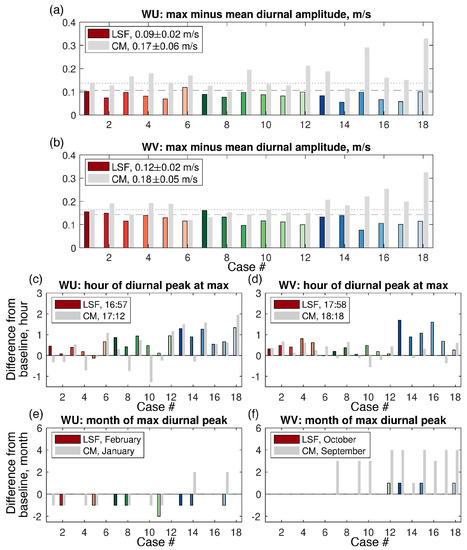
Figure 6.
As in Figure 5, now showing: (a,b) maximum minus mean diurnal amplitude during the year; (c–f) the differences between the estimates from decimated timeseries (using LSF versus CM method) and the baseline for (c,d) the hour of the diurnal peak in the month when the diurnal signal is maximum, (e,f) the month of the year when the diurnal amplitude is maximum. Panels (a,c,e) are for zonal wind, and panels (b,d,f) for meridional wind. In panels (c–f), the legend indicates the baseline estimates.
5. Annual Modulation of Diurnal Variability in the Tropical Ocean
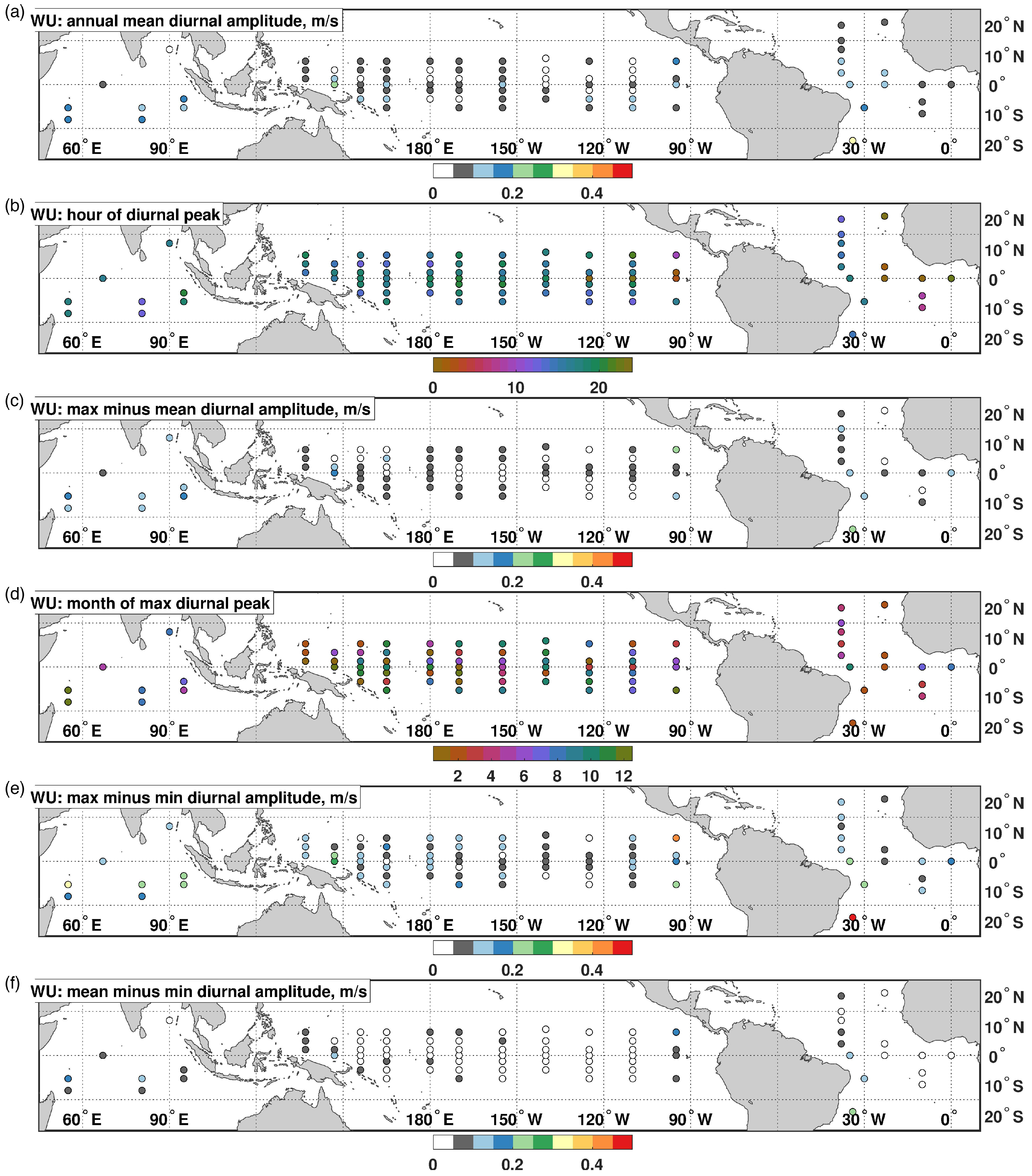
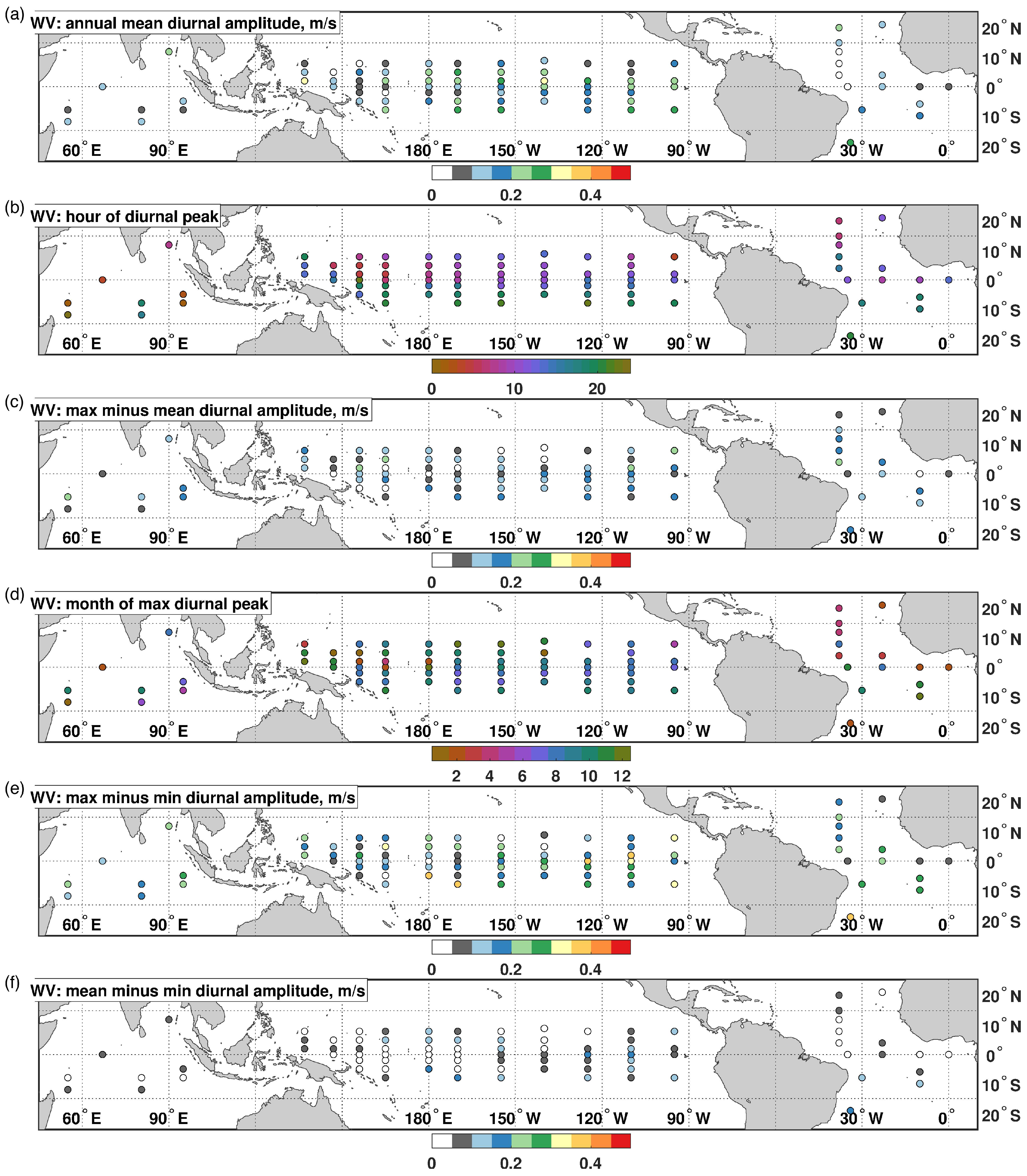
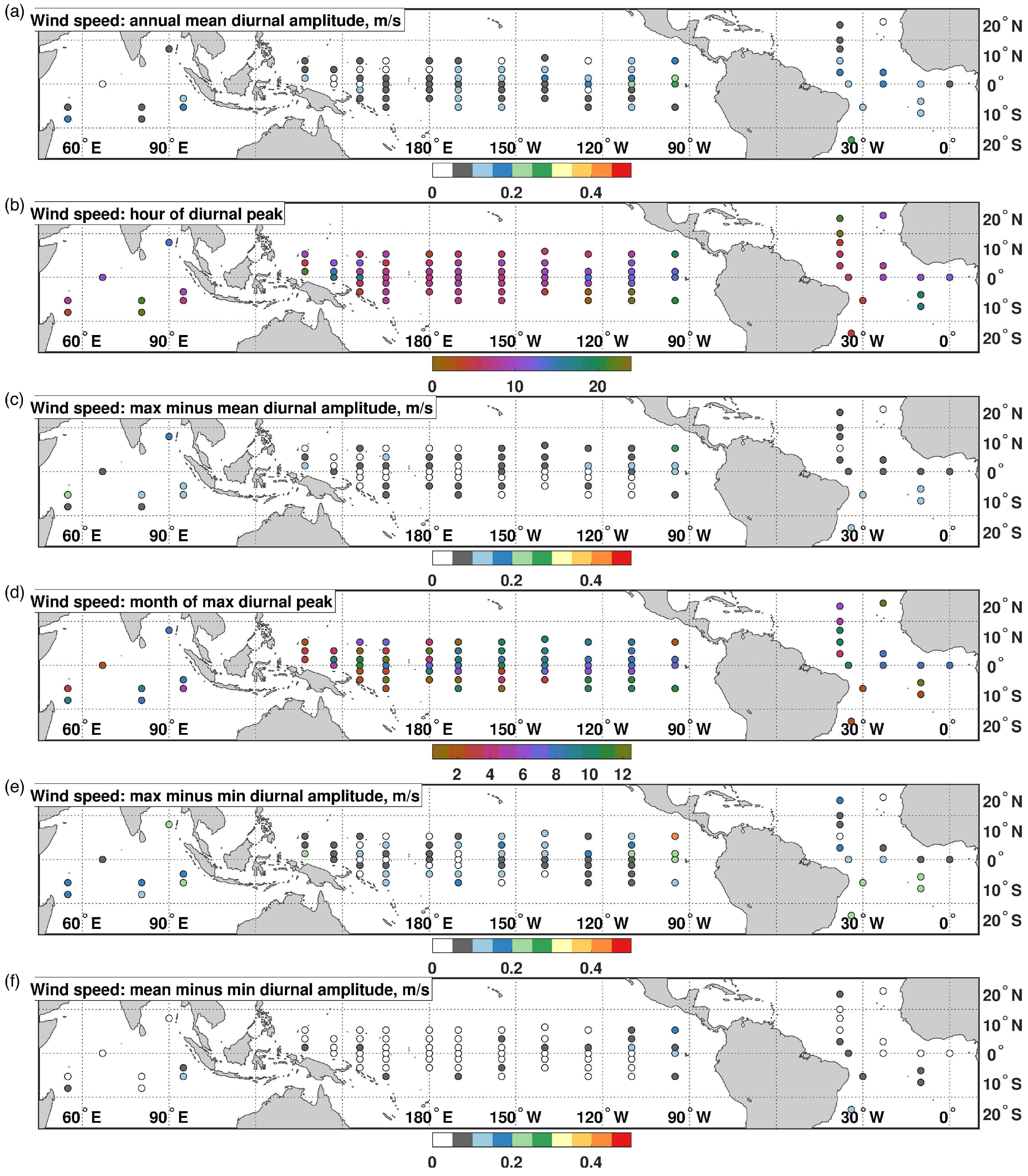
In this section, we first characterize the annual mean diurnal amplitude and phase (as hour of the diurnal peak) of near-surface winds in the tropical ocean from mooring data (e.g., panels (a,b) in Figure 7, Figure 8 and Figure 9). Then, we characterize how this variability changes in different months of the year. The annual modulation of diurnal variability is described in terms of differences between: maximum diurnal amplitude in the year minus annual mean diurnal amplitude (e.g., panel (c) in Figure 7, Figure 8 and Figure 9); annual mean minus minimum diurnal amplitude in the year (e.g., panel (f) in Figure 7, Figure 8 and Figure 9); maximum minus minimum diurnal amplitude in the year (e.g., panel (e) in Figure 7, Figure 8 and Figure 9). The first two metrics are useful to see the asymmetry in how much maximum and minimum diurnal amplitudes can differ from the annual mean value. The maximum minus minimum diurnal amplitude matrix is the sum of the other two and is included to provide a quick visualization of diurnal variability changes throughout the year. We also show the month when the diurnal amplitude is largest in the year (e.g., panel (d) in Figure 7, Figure 8 and Figure 9). We focus on results from the LSF method (now applied to all the sites in red in Figure 1), as LSF can isolate annual modulation of diurnal variability from other signals, in addition to showing overall greater robustness compared to CM (Section 4). For reference, we will also summarize in Figure 10 and Figure 11 how LSF-based estimates that include the combined effect of annual and semi-annual modulation compare with CM-based estimates (which are representative of seasonal modulation).
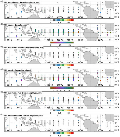
Figure 7.
Zonal near-surface wind (WU) in the tropical ocean: (a) annual mean diurnal amplitude; (b) hour of the annual mean diurnal peak in local time; (c) difference between the maximum diurnal amplitude in the year and the annual mean diurnal amplitude in panel (a); (d) month of the year when the diurnal amplitude is maximum; (e) difference between maximum and minimum diurnal amplitude in the year; (f) difference between the annual mean diurnal amplitude in panel (a) and the minimum diurnal amplitude in the year. Results are for the LSF method.
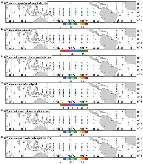
Figure 8.
Same as Figure 7, now for meridional near-surface wind (WV).
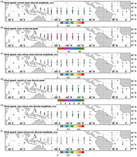
Figure 9.
Same as Figure 7, now for near-surface wind speed.
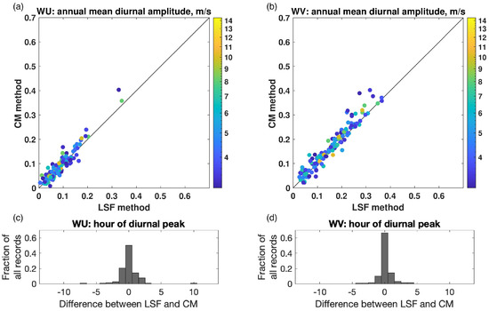
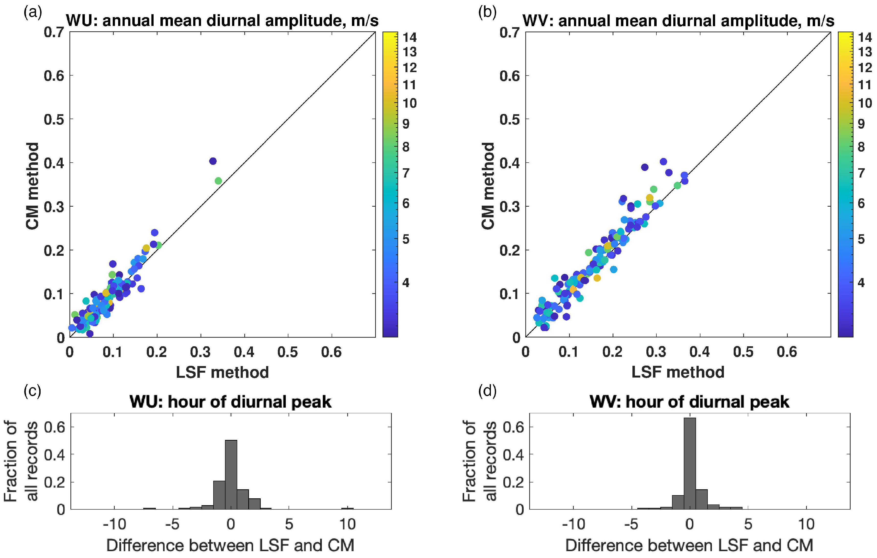
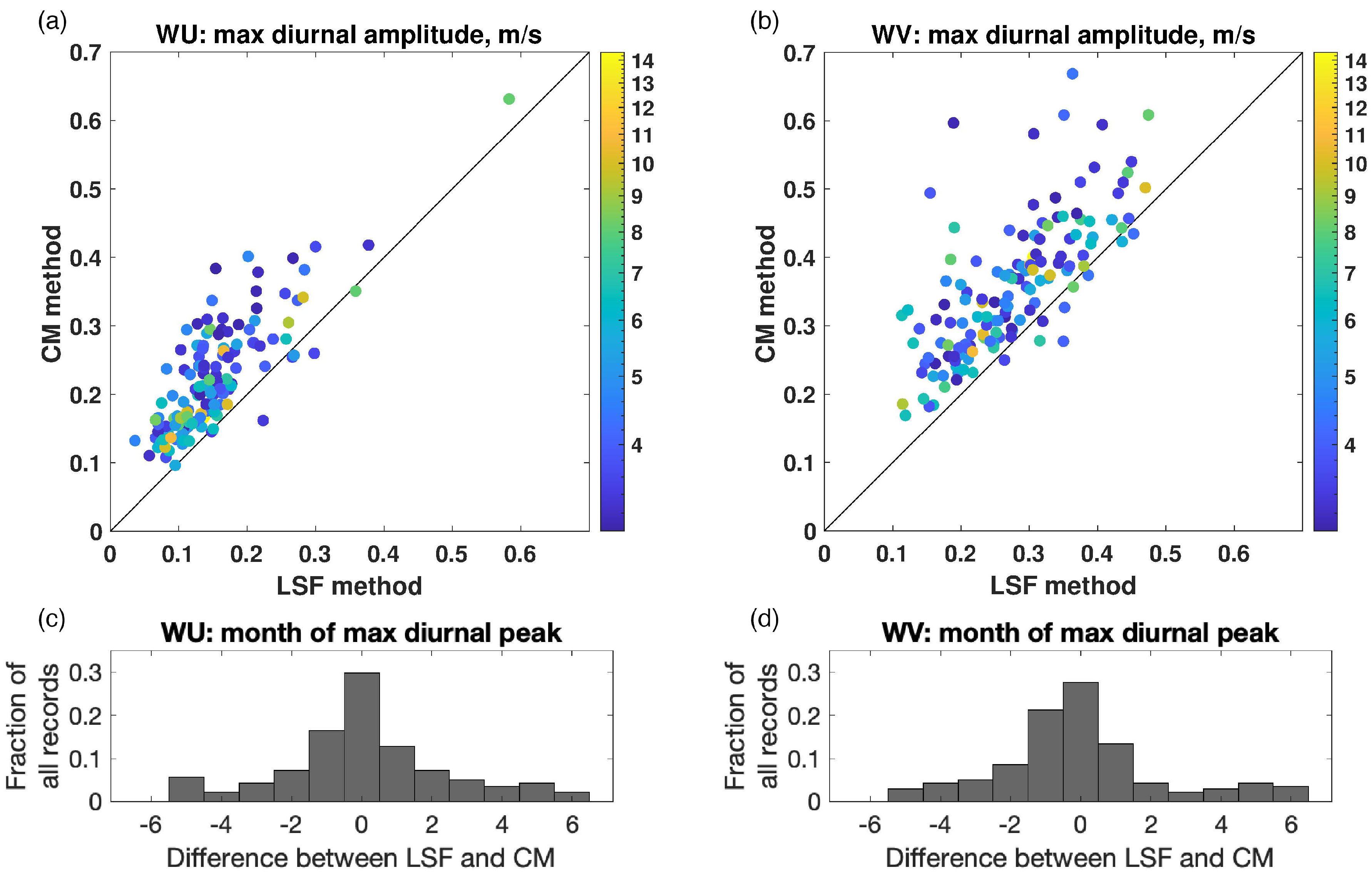
Figure 10.
Zonal (WU, panels (a,c)) and meridional (WV, panels (b,d)) surface wind in the tropical ocean: comparison between the LSF versus CM method. Panels (a,b) are for the annual mean diurnal amplitude: the LSF estimate is on the horizontal axis, the CM on the vertical, and the color indicates the length of the data record (in years) used in the analysis. Panels (c,d) are for the differences (between the LSF and CM method) in hour of the annual mean diurnal peak: the vertical axis shows the fraction of all records that are characterized by each difference (differences are on the horizontal axis). All results are based on observations measured at the mooring locations in red in Figure 1.
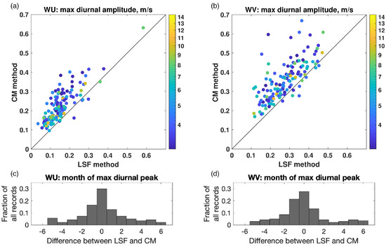
Figure 11.
As in Figure 10, now showing (a,b) the maximum diurnal amplitude during the year for (a) WU and (b) WV (length of the data record in color, in years); (c,d) fraction of all records by LSF versus CM differences in the month of the year when the diurnal amplitude is maximum for (c) WU and (d) WV. For this comparison with CM, LSF includes harmonics for both the annual and semiannual modulation, as CM does not isolate the annual modulation.
Results for the annual mean amplitude and phase of diurnal winds in the tropical ocean (panels (a,b) in Figure 7, Figure 8 and Figure 9) are consistent with previous studies (for those regions where previous studies are available, see, e.g., in [2,4,5,15]). Here, we quantify the amplitude of the diurnal cycle from moorings in each of the three ocean basins and observe an overall stronger diurnal amplitude in meridional winds (compared to zonal winds; Figure 8a versus Figure 7a), with larger values of the meridional diurnal component in the Pacific Ocean compared to the other basins. As documented in previous studies based on shorter mooring records (see, e.g., in [2,4]), zonal winds in the Pacific display overall a stronger semi-diurnal than diurnal variability (not shown). The diurnal signal in zonal winds is stronger in the Atlantic and Indian Oceans (compared to the Pacific; Figure 7a). Here, for some of the moorings, this signal is even stronger than that of meridional winds. Annual-mean diurnal winds in the zonal direction are particularly weak for moorings between 140°W and 110°W, north of 2°S (as indicated by the prevalence of white circles in the region in Figure 7a). The CM and LSF methods overall agree with one another for the estimate of the annual mean diurnal amplitude, regardless of the record length (Figure 10a,b). This is not always the case for the hour of the diurnal peak, yet results from the two methods differ by no more than one hour for most of the records (Figure 10c,d). For zonal winds, the diurnal peak is observed in the afternoon/evening throughout the tropics, except for some of the moorings in the eastern Pacific and Atlantic Oceans, where a peak is observed in the morning (Figure 7b). Diurnal variations in meridional wind tend to be out of phase north and south of the equator in the tropical Pacific (e.g., [4], plus Figure 8b here), with implications for wind divergence at the equator. This behavior is not observed as clearly in other basins, where we have a smaller number of moorings and fewer records suitable for our analysis.
Due to annual modulation of diurnal variability, the annual mean diurnal cycle may be different from the diurnal cycle observed in any given month of the year. The largest differences in diurnal amplitude across months and between individual months and the annual mean are found in the eastern to central Pacific for the meridional wind component, in addition to sites in the Atlantic and Indian basins (Figure 8c,e,f).
For zonal winds, the largest differences across months and between individual months and the annual mean are found in the Indian Ocean and at a few moorings in the eastern and western Pacific and Atlantic. While diurnal variability in meridional wind peaks between June and November in most of the tropical Pacific, the peak is earlier in the year in the western Pacific and at many of the sites in the Atlantic basin (Figure 8d).
For zonal wind, there is more spatial variability to the timing of the maximum diurnal variability in the year (Figure 7d). The annual modulation of diurnal variability is overall smaller for zonal winds (Figure 7c,e,f), although there are exceptions: for several sites, the maximum diurnal signal in the year is at least twice as large as the annual mean diurnal amplitude (see moorings where the difference between maximum and mean diurnal cycle in Figure 7c is similar to or larger than the amplitude in Figure 7a).
The estimated peak in diurnal variability during the year is larger with CM than LSF, with the longest records yielding the smallest differences between the two methods (Figure 11a,b). The two methods agree more closely for the month of the year when the diurnal signal reaches a maximum, with differences within a month for many of the records (Figure 11c,d).
The relationship between ocean wind speed and its zonal and meridional wind components is nonlinear. For the mooring data, the largest annual mean diurnal amplitude for wind speeds occurs in the eastern tropical Pacific and western Atlantic, as shown in Figure 9a. The lowest values are found in the western Pacific. Diurnal wind speed peaks in the morning in most of the tropics with some exceptions in all basins (Figure 9b). As an example, in the tropical Pacific, diurnal peaks in the afternoon/evening are observed west of 160°E and east of 130°W.
The largest differences in diurnal amplitude across months and between individual months and the annual mean are found, for wind speed, in the Indian Ocean and eastern tropical Pacific (Figure 9c,e,f). Diurnal variability in wind speed is generally largest in months from June to November, except in, e.g., the western Pacific and Atlantic when diurnal variability peaks early in the year (Figure 9d). Finally, the weakest annual modulation of diurnal variability (i.e., the smallest difference between the maximum and minimum diurnal amplitude in the year) is observed in the western Pacific and south of the equator between 140°W and 110°W (Figure 9e).
6. Summary and Conclusions
This study describes how the diurnal cycle in surface winds changes in different months of the year over the tropical ocean. We analyze high-frequency observations from the tropical mooring array and use the method of least squares to perform harmonic analysis. The model we fit to the data is designed to extract the diurnal signal and its annual modulation in finite time series with missing values. We compare our method with compositing approaches used in previous studies in which raw data are binned into 1-h bins and a diurnal and a semidiurnal cycle are fitted to the resulting composites. Both methods show that the largest amplitude in the annual mean diurnal cycle of surface winds is in meridional winds, consistent with previous studies (see, e.g., in [4] for the Tropical Pacific). Zonal winds show overall stronger semi-diurnal than diurnal variability. While the diurnal amplitude in meridional winds peaks in the tropical Pacific, diurnal variability in zonal winds is overall weaker there compared to other basins. These variations in zonal and meridional winds result from a variety of mechanisms (including diurnal pressure gradients) and combine to produce a diurnal cycle in wind speed that has a peak in the morning in a large region of the central tropical Pacific and western Atlantic. Atmospheric boundary layer instabilities and resulting vertical exchanges of momentum may contribute to observed diurnal variability, as well as diurnal variability in tropical oceanic convective precipitation [38,39]. Exploring these links is beyond the scope of our analysis.
As drivers of diurnal variability in surface winds (e.g., changes in temperature and pressure gradients) are subject to an annual cycle, annual modulation of diurnal winds is observed and is stronger for meridional winds. The diurnal signal in meridional winds is strongest between June and November in most of the tropical Pacific, tropical south Atlantic, and Indian Oceans, with the largest differences between individual months and the annual mean in the eastern to central Pacific. Annual modulation of diurnal variability is also observed in the tropical north Atlantic where the diurnal amplitude peaks earlier in the year.
Quantifying annual modulation of the diurnal signal can help better understand diurnal variability in surface winds, including relevant mechanisms and implications for air–sea interactions. Furthermore, it is useful to improve climate records of surface winds from satellite data, as it helps to cross-calibrate wind-measuring satellites that have different equator crossing times. The signal measured by satellites is effectively a weighted spatial average over a footprint (e.g., 20–40 km), while moorings provide point measurements. This should be taken into account when using results for diurnal variability in surface winds based on in situ observations to improve satellite-based estimates, as any spatial structure within the footprint is suppressed in satellite measurements. Furthermore, while satellite wind observations are sensitive to the winds at the ocean surface (i.e., the wind-induced ocean surface roughness), the satellite wind estimates are referenced to a standard 10 m height, adding uncertainty due to unknown atmospheric stratification (among other factors). The GTMBA moorings measure winds at 4 m above the ocean surface. To compare satellite and mooring observations, they all need to be adjusted to the same height above the ocean surface, introducing uncertainty into the comparison. In addition, the moorings measure the actual wind while the satellites are sensitive to the wind that is relative to the surface current. Even with these caveats, analyses based on mooring data are helpful in characterizing diurnal wind and its annual modulation and in testing sampling scenarios in order to identify sampling requirements for wind-measuring satellites to capture this signal. The framework presented here can help investigate how well different aspects of the annual modulation of the diurnal signal (e.g., maximum diurnal peak and when it occurs in the year) are captured by time series of different lengths, temporal resolution and sampling time in the day. This framework can guide selections of sampling strategies adapted for the targeted quantities. Our method based on harmonic analysis provides a more robust estimate of the month when diurnal variability peaks, compared to binning the raw time series, across sampling scenarios. These sampling scenarios include sparse, satellite-like measurements that make it difficult to estimate annual modulation especially when a semi-diurnal signal is present and/or the record is only 3–5 year long. Estimating the annual modulation of the diurnal signal implies resolving peaks in energy both at the diurnal frequency (i.e., ) and at [35]. To achieve the former, sampling at least 6 times per day is helpful, as observed winds also include semidiurnal variability. (Sampling 4 times per day would be at the Nyquist frequency of the semi-diurnal signal, and phase information cannot be determined at the Nyquist frequency.) To achieve the latter, a frequency resolution is required that clearly differentiates and . For this, it is helpful to resolve multiple frequencies between and both and . This implies a length of the time series of at least 3 years [35]. The choice of sampling strategy should be finalized based on what the target is. As an example, our results show that the LSF method can capture (within a month) the month of the maximum diurnal peak in a decimated 3-year time series sampled every 4 h from wind observations at 30°W, 8°S (Figure 6e,f).
Author Contributions
Conceptualization, D.G., S.T.G. and B.D.C.; methodology, D.G., S.T.G., A.C.S. and B.D.C.; software, D.G. and B.D.C.; validation, D.G. and F.J.T.; formal analysis, D.G.; investigation, D.G., D.N., F.J.T. and S.H.-V.; data curation, D.G.; writing—original draft preparation, D.G.; writing—review and editing, all authors; visualization, D.G.; supervision, D.G. and S.T.G.; project administration, D.G. and S.T.G.; funding acquisition, D.G., A.C.S. and S.T.G. All authors have read and agreed to the published version of the manuscript.
Funding
This research was funded by NASA Ocean Vector Winds Science Team (awards NNX14AO78G and 80NSSC19K0059). B.C. was funded by NOAA Grant NA18OAR4310403. A.C.S. was funded by NOAA CVP grant number NA18OAR4310405 and ONR, United States (N00014-17-S-B001). F.J.T. and S.H.-V. acknowledge support from NASA’s Making Earth Science Data Records for Use in Research Environments (MEaSUREs) program.
Data Availability Statement
Data used in this study are made available by the Global Tropical Moored Buoy Array Project Office of NOAA/PMEL at https://www.pmel.noaa.gov/gtmba/, accessed on 14 July 2020.
Acknowledgments
The work by F.J.T. and S.H.-V. was carried out at the Jet Propulsion Laboratory, California Institute of Technology, under a contract with the National Aeronautics and Space Administration. The discussions with (and related work carried out by) Thomas Kilpatrick and other members of the NASA Ocean Vector Winds science team contributed to the explanation of the results. We thank Mark Bourassa for his leadership of the NASA Ocean Vector Winds science team. We would also like to thank the anonymous reviewers for their thoughtful feedback on this manuscript.
Conflicts of Interest
The authors declare no conflict of interest.
Abbreviations
The following abbreviations are used in this manuscript:
| GTMBA | Global Tropical Moored Buoy Array |
| LSF | least-squares fit method (in this study) based on harmonic analysis |
| CM | composite method in this study |
| WU | zonal near-surface wind |
| WV | meridional near-surface wind |
References
- Deser, C.; Smith, C.A. Diurnal and Semidiurnal Variations of the Surface Wind Field over the Tropical Pacific Ocean. J. Clim. 1998, 11, 1730–1748. [Google Scholar] [CrossRef]
- Dai, A.; Deser, C. Diurnal and semidiurnal variations in global suface wind divergence fields. J. Geophys. Res. 1999, 104, 31109–31125. [Google Scholar] [CrossRef] [Green Version]
- Dai, A.; Trenberth, K.E. The Diurnal Cycle and Its Depiction in the Community Climate System Model. J. Clim. 2004, 17, 930–951. [Google Scholar] [CrossRef]
- Ueyama, R.; Deser, C. A Climatology of Diurnal and Semidiurnal Surface Wind Variations over the Tropical Pacific Ocean Based on the Tropical Atmosphere Ocean Moored Buoy Array. J. Clim. 2008, 21, 593–607. [Google Scholar] [CrossRef] [Green Version]
- Gille, S.T.; Llewellyn Smith, S.G.; Statom, N.M. Global Observations of the Land Breeze. Geophys. Res. Lett. 2005, 32. [Google Scholar] [CrossRef] [Green Version]
- Williams, C.R.; Avery, S.K.; McAfee, J.R.; Gage, K.S. Comparison of observed diurnal and semidiurnal tropospheric winds at Christmas Island with tidal theory. Geophys. Res. Lett. 1992, 19, 1471–1474. [Google Scholar] [CrossRef]
- Aspliden, C. Diurnal and semidiurnal low-level wind cycles over a tropical island. Bound.-Layer Meteorol. 1977, 12, 187–199. [Google Scholar] [CrossRef]
- Deser, C. Daily surface wind variations over the equatorial Pacific Ocean. J. Geophys. Res. Atmos. 1994, 99, 23071–23078. [Google Scholar] [CrossRef] [Green Version]
- Moum, J.N.; Nash, J.D.; Smyth, W.D. Narrowband high-frequency oscillations at the equator. Part I: Interpretation as shear instabilities. J. Phys. Oceanogr. 2011, 41, 397–411. [Google Scholar] [CrossRef]
- Ruppert, J.H., Jr.; Johnson, R.H. Diurnally modulated cumulus moistening in the preonset stage of the Madden–Julian oscillation during DYNAMO. J. Atmos. Sci. 2015, 72, 1622–1647. [Google Scholar] [CrossRef] [Green Version]
- Ciesielski, P.E.; Johnson, R.H.; Schubert, W.H.; Ruppert, J.H., Jr. Diurnal cycle of the ITCZ in DYNAMO. J. Clim. 2018, 31, 4543–4562. [Google Scholar] [CrossRef]
- Chen, S.S.; Houze, R.A., Jr. Diurnal variation and life-cycle of deep convective systems over the tropical Pacific warm pool. Q. J. R. Meteorol. Soc. 1997, 123, 357–388. [Google Scholar] [CrossRef]
- Weller, R.; Anderson, S. Surface meteorology and air-sea fluxes in the western equatorial Pacific warm pool during the TOGA Coupled Ocean-Atmosphere Response Experiment. J. Clim. 1996, 9, 1959–1990. [Google Scholar] [CrossRef] [Green Version]
- Cronin, M.F.; Kessler, W.S. Seasonal and interannual modulation of mixed layer variability at 0, 110 W. Deep. Sea Res. Part I Oceanogr. Res. Pap. 2002, 49, 1–17. [Google Scholar] [CrossRef]
- Turk, F.J.; Hristova-Veleva, S.; Giglio, D. Examination of the Daily Cycle Wind Vector Modes of Variability from the Constellation of Microwave Scatterometers and Radiometers. Remote Sens. 2021, 13, 141. [Google Scholar] [CrossRef]
- Bond, N.A.; McPhaden, M.J. An indirect estimate of the diurnal cycle in upper ocean turbulent heat fluxes at the equator, 140 W. J. Geophys. Res. Ocean. 1995, 100, 18369–18378. [Google Scholar] [CrossRef]
- Moum, J.N.; Caldwell, D.R.; Paulson, C.A. Mixing in the equatorial surface layer and thermocline. J. Geophys. Res. Ocean. 1989, 94, 2005–2022. [Google Scholar] [CrossRef]
- Chereskin, T.K.; Moum, J.N.; Stabeno, P.J.; Caldwell, D.R.; Paulson, C.A.; Regier, L.A.; Halpern, D. Fine-scale variability at 140° W in the Equatorial Pacific. J. Geophys. Res. 1986, 91, 12887–12897. [Google Scholar] [CrossRef] [Green Version]
- Moulin, A.J.; Moum, J.N.; Shroyer, E.L. Evolution of Turbulence in the Diurnal Warm Layer. J. Phys. Oceanogr. 2018, 48, 383–396. [Google Scholar] [CrossRef]
- Wentz, F.J.; Ricciardulli, L.; Ernesto Rodriguez, B.W.S.; Bourassa, M.A.; Long, D.G.; Hoffman, R.N.; Stoffelen, A.; Verhoef, A.; O’Neill, L.W.; Farrar, J.T.; et al. Evaluating and Extending the Ocean Wind Climate Data Record. IEEE J. Sel. Top. Appl. Earth Obs. Remote Sens. 2017, 10, 2165–2185. [Google Scholar] [CrossRef] [PubMed] [Green Version]
- Chang, P. The Ocean Surface Vector Wind Constellation: Status, Health and Future? Available online: https://mdc.coaps.fsu.edu/scatterometry/meeting/docs/2017/docs/Tuesday/morning/FirstSession/905_PCHANG_IOWVST_OSVW-VC_02MAY2017_final.pdf (accessed on 14 July 2020).
- Gille, S.T.; Llewellyn Smith, S.G.; Lee, S.M. Measuring the Sea Breeze from QuikSCAT Scatterometry. Geophys. Res. Lett. 2003, 30. [Google Scholar] [CrossRef] [Green Version]
- Simpson, J.E. Sea Breeze and Local Wind; Cambridge University Press: Cambridge, UK, 1994. [Google Scholar]
- Miller, S.T.K.; Keim, B.D.; Talbot, R.W.; Mao, H. Sea Breeze: Structure, Forecasting, and Impacts. Rev. Geophys. 2003, 41. [Google Scholar] [CrossRef] [Green Version]
- Wood, R.; Koehler, M.; Bennartz, R.; O’Dell, C. The diurnal cycle of surface divergence over the global oceans. Q. J. R. Meteorol. Soc. 2009, 135, 1484–1493. [Google Scholar] [CrossRef]
- Gille, S.T.; Llewellyn Smith, S.G. When land breezes collide: Converging diurnal winds over small bodies of water. Q. J. R. Meteorol. Soc. 2014, 140, 2573–2581. [Google Scholar] [CrossRef] [Green Version]
- Hyder, P.; Simpson, J.H.; Xing, J.; Gille, S.T. Observations over an annual cycle and simulations of wind-forced oscillations near the critical latitude for diurnal-inertial resonance. Cont. Shelf Res. 2011, 31, 1576–1591. [Google Scholar] [CrossRef]
- McPhaden, M.J.; Ando, K.; Bourles, B.; Freitag, H.; Lumpkin, R.; Masumoto, Y.; Murty, V.; Nobre, P.; Ravichandran, M.; Vialard, J.; et al. The global tropical moored buoy array. Proc. Ocean. 2010, 9, 668–682. [Google Scholar]
- Hayes, S.; Mangum, L.; Picaut, J.; Sumi, A.; Takeuchi, K. TOGA-TAO: A moored array for real-time measurements in the tropical Pacific Ocean. Bull. Am. Meteorol. Soc. 1991, 72, 339–347. [Google Scholar] [CrossRef] [Green Version]
- Servain, J.; Busalacchi, A.J.; McPhaden, M.J.; Moura, A.D.; Reverdin, G.; Vianna, M.; Zebiak, S.E. A pilot research moored array in the tropical Atlantic (PIRATA). Bull. Am. Meteorol. Soc. 1998, 79, 2019–2032. [Google Scholar] [CrossRef] [Green Version]
- McPhaden, M.J.; Meyers, G.; Ando, K.; Masumoto, Y.; Murty, V.; Ravichandran, M.; Syamsudin, F.; Vialard, J.; Yu, L.; Yu, W. RAMA: The research moored array for African–Asian–Australian monsoon analysis and prediction. Bull. Am. Meteorol. Soc. 2009, 90, 459–480. [Google Scholar] [CrossRef] [Green Version]
- Milburn, H.B.; McLain, P.D.; Meinig, C. ATLAS buoy-reengineered for the next decade. In Proceedings of the OCEANS 96 MTS/IEEE Conference Proceedings. The Coastal Ocean-Prospects for the 21st Century, Fort Lauderdale, FL, USA, 23–26 September 1996; Volume 2, pp. 698–702. [Google Scholar]
- Gille, S.T. Diurnally Varying Wind Forcing and Upper Ocean Temperature: Implications for the Ocean Mixed Layer. In Proceedings of the 16th Conference on Air-Sea Interaction, Phoenix, AZ, USA, 11–15 January 2009. [Google Scholar]
- Roemmich, D.; Gilson, J. The 2004–2008 mean and annual cycle of temperature, salinity, and steric height in the global ocean from the Argo Program. Prog. Oceanogr. 2009, 82, 81–100. [Google Scholar] [CrossRef]
- Bracewell, R.N. The Fourier Transform and Its Applications, 2nd ed.; McGraw-Hill: New York, NY, USA, 1978. [Google Scholar]
- Wunsch, C. The Ocean Circulation Inverse Problem; Cambridge University Press: Cambridge, UK, 1996; p. 437. [Google Scholar]
- Von Storch, H.; Zwiers, F.W. Statistical Analysis in Climate Research; Cambridge University Press: Cambridge, UK, 1999. [Google Scholar] [CrossRef] [Green Version]
- Yang, S.; Smith, E.A. Mechanisms for Diurnal Variability of Global Tropical Rainfall Observed from TRMM. J. Clim. 2006, 19, 5190–5226. [Google Scholar] [CrossRef] [Green Version]
- Kilpatrick, T.; Xie, S.P.; Nasuno, T. Diurnal Convection-Wind Coupling in the Bay of Bengal. J. Geophys. Res. Atmos. 2017, 122, 9705–9720. [Google Scholar] [CrossRef]

Publisher’s Note: MDPI stays neutral with regard to jurisdictional claims in published maps and institutional affiliations. |
© 2022 by the authors. Licensee MDPI, Basel, Switzerland. This article is an open access article distributed under the terms and conditions of the Creative Commons Attribution (CC BY) license (https://creativecommons.org/licenses/by/4.0/).