Mapping Phragmites australis Aboveground Biomass in the Momoge Wetland Ramsar Site Based on Sentinel-1/2 Images

Abstract

Phragmites australis (P. australis) is one of the most important plant species found in wetland ecosystems, and its aboveground biomass (AGB) is a key indicator for assessing the quality or health of a wetland site. In this study, we combined Sentinel-1/2 images and field observation data collected in 2020, to delineate the distribution of P. australis in the Momoge Ramsar Wetland site by using a random forest method, and further, to estimate AGB by comparing multiple linear regression models. The results showed that the overall classification accuracy of P. australis using the random forest method was 89.13% and the P. australis area in the site was 135.74 km² in 2020. Among various remote sensing variables, the largest correlation coefficient was observed between dry weight of AGB of P. australis and Sentinel-2 red edge B₇, and between fresh weight of P. australis AGB and red edge B₅. The optimal models for estimating dry and fresh weight of P. australis AGB were multiple linear regression models, with an accuracy of 75.4% and 69.2%, respectively. In 2020, it was estimated that the total fresh weight of P. australis AGB in this Ramsar site was 21.2 × 10⁷ kg and the total dry weight was 7.2 × 10⁷ kg. The larger weight of P. australis AGB was identified mainly at central and western sites. The application of Sentinel-2 red-edge band for AGB estimation can significantly improve the model estimation accuracy. The findings of this study will provide a scientific basis for the management and protection of wetland ecosystems and sustainable utilization of P. australis resources.

1. Introduction

Wetlands are valuable ecosystems of the earth, with multiple unique functions and services. They not only provide humans with a large amount of raw material and water resources, but also maintain ecological balance, and protect biodiversity and rare species resources [1,2]. Phragmites australis (P. australis) is a typical wetland plant community type that is important in wetlands internationally. It plays an important role in the functions and services of the wetland ecosystem, such as sequestering carbon and providing shelter for migrating waterbirds [3,4]. P. australis is also an important biological resource. However, excessive utilization of P. australis resources may damage the sustainable management of a wetland ecosystem [5,6]. Therefore, the accurate extraction of P. australis distribution information and the precise weight estimation of P. australis aboveground biomass (AGB) has enormous scientific significance and practical value [7].

In order to invert the biomass more accurately, it is very important to obtain the fine spatial pattern of wetland communities, which can also be highly informative for better management of wetland ecosystems [8,9]. Currently, there are many studies on wetland classification [10,11], but the accuracy of wetland classification needs to be improved due to the wide distribution of wetland vegetation, complex community composition, high spectral similarity, and insignificant variation in the characteristics of different vegetation [12]. Refining classification on a community scale and extracting single community data can effectively improve the accuracy of wetland mapping and biomass inversion, and achieve a clearer understanding and far-reaching impact on wetland landscape patterns [13]. Machine learning is an efficient method for extracting wetland vegetation at community scale [14]. As an important branch of machine learning methods, random forest classification is an accurate and efficient method for wetland information gathering [15]. Using a random forest algorithm to extract wetland vegetative information can effectively improve classification accuracy and help analyze spatial patterns of wetlands.

A remote sensing data source is an important prerequisite for achieving reliable wetland classification. Due to the complex community composition of wetland vegetation and intensive disturbance from water bodies, traditional remote sensing images with low spatial resolution, such as Landsat and MODIS, are often not ideal for fine-scale classification [16,17,18]. Sentinel-2 satellite images have a higher spectral and spatio-temporal resolution in optical images, and contain three unique bands within the red-edge range, giving Sentinel-2 an advantage in wetland plant identification [19,20]. Radar images provided by Sentinel-1 satellites allow for stable periodic data acquisition. They contain characteristics of all-day and all-weather capabilities, which can effectively ameliorate the shortfall in Sentinel-2 optical images, which are often covered by cloud and fog [21]. The spectral reflectance of wetland vegetation has a more distinctive feature in areas with water coverage, especially in the red-edge band of Sentinel-2. The reflectance of typical wetland vegetation is generally lower than that of other terrestrial vegetation [22]. Radar images may be unaffected by atmospheric illumination and clouds, and can be used together with Sentinel-2 to obtain information on different types of wetland vegetation [23,24]. Therefore, compared with using a single image source, combining the red-edge and radar features of both Sentinel sensors could improve the accuracy of wetland vegetation identification [25,26].

Nowadays, the remote sensing-based models used to estimate the weight of wetland vegetation AGB can be categorized as optical remote sensing models, radar models, and multi-source remote sensing collaborative models. There are two main methods used in the estimation of wetland vegetation AGB based on remote sensing models, namely, machine learning and linear regression [27]. Although machine learning can achieve spatial prediction of AGB, it cannot explain the relationships satisfactorily [28], and the estimation results cannot ensure high precision [29]. The linear regression model, combined with multiple variables, can effectively describe the complex linear relationship between AGB of P. australis and remotely sensed variables, and the inversion accuracy is high for small areas [30].

The Momoge Wetland Ramsar site (No. 2188) is an internationally important wetland in northeastern China. It is an important breeding ground and habitat for migratory birds, and plays an important role in biodiversity conservation and climate regulation. There are many plant species in the Ramsar site, with the P. australis community occupying the largest proportion. Analysis of P. australis community distribution and AGB estimation can help to better manage the overall wetland environment [31,32]. The lack of high-precision information on the spatial distribution of P. australis and AGB estimation has limited the conservation and asset estimation of the wetland. To better manage the Ramsar site, we used a random forest algorithm and regression models in combination with Sentinel-1 and Sentinel-2 remote sensing images, to depict P. australis distribution and estimate its AGB. We tested the effectiveness of multiple regression models for accurately retrieving fresh and dry weight of P. australis AGB. The results of this study are expected to improve the management, conservation, and sustainable utilization of P. australis resources.

2. Materials and Methods

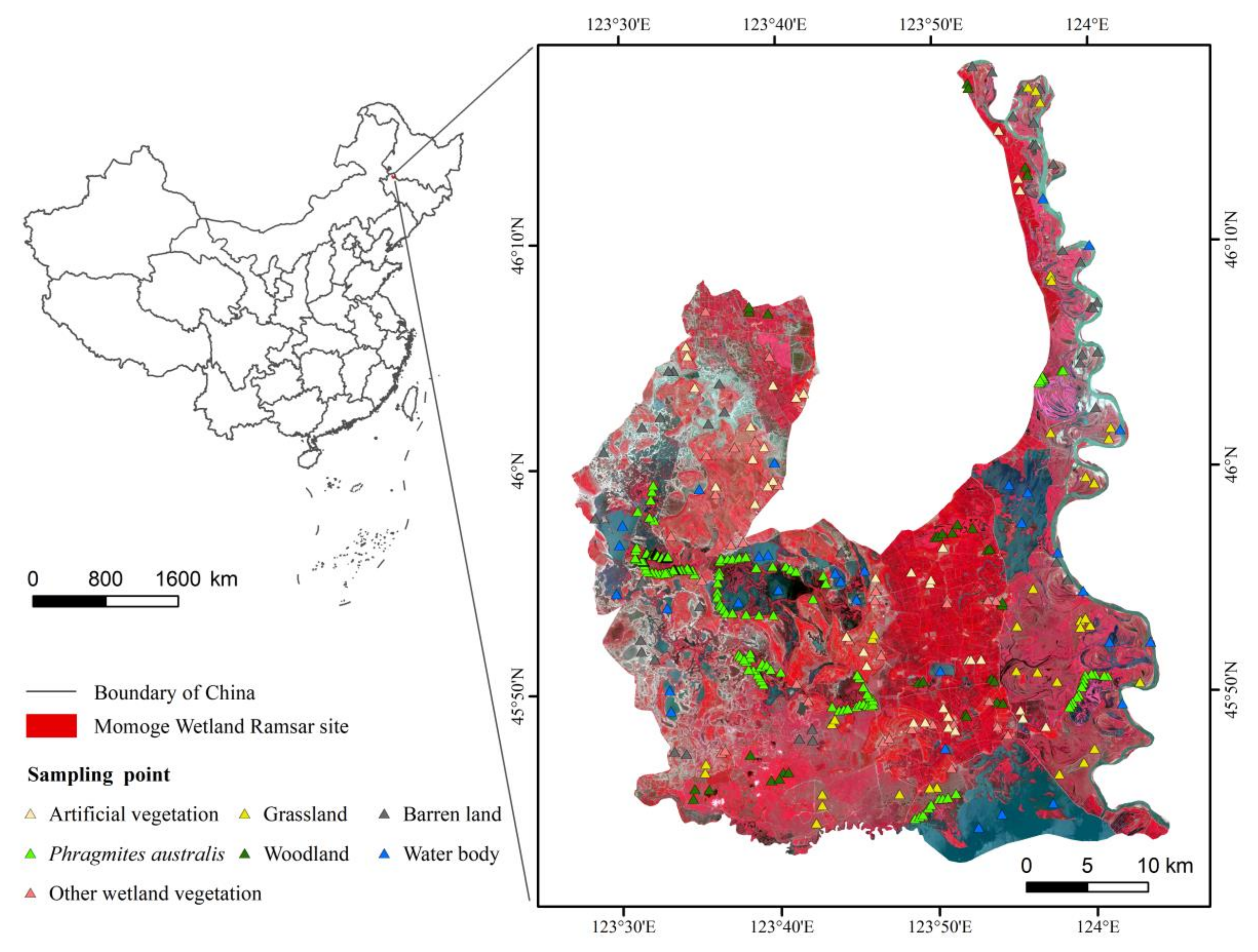
2.1. Study Area

The Momoge Wetland, located in the western Jilin Province of China (Figure 1), spans 45°42∲ N to 46°18∲ N and 123°27∲ E to 124°4∲ E, and covers a total area of about 1440 km². As an important stopover site for the migration of Grus leucogeranus and other important water birds, the reserve was designated in the List of Wetlands of International Importance in 2013 [33]. The reserve is flat with a relative elevation difference of only 2–10 m. This region belongs to the temperate continental monsoon climate, with strong winds and drought in spring, heat and rain in summer, cool and dry conditions in autumn, and cold and snow in winter. The annual average temperature is 5 °C, the annual average evapotranspiration is 1500 mm, and the annual average precipitation is 385 mm [34]. The Nenjiang River system flows through the east portion for 111.5 km, with a drainage area of more than 30,000 hectares. The region is rich in plant and animal resources, with about 600 species of seed plants, and the dominant wetland vegetation is P. australis [35]. There are abundant wildlife species, including 298 species of birds [36].

2.2. Datasets

2.2.1. Sentinel-1/2 Image Selection and Processing

In this study, Sentinel-1 IW GRD (ground range detected, GRD) images and Sentinel-2 L1C images were selected as remote sensing data sources. These images were acquired on 23 July and 15 July 2020, respectively, and were downloaded from the European Space Agency (ESA) website (https://earth.esa.int/web/guest/home (accessed on 15 July 2020 and 23 July 2020)). The Sentinel-1 data were preprocessed by orbit correction, resampling, and clipping to obtain the radar data of VV and VH polarization backscattering coefficients for the study area. The 10 bands of Sentinel-2 L1C were obtained after atmospheric cirrus cloud correction and resampled to 10 m resolution (

Table 1. Description of the Sentinel-1/2 images used.

Acquisition Date: 15 July 2020		Acquisition Date: 23 July 2020
Sentinel-2 Band	Spatial Resolution (m)	Sentinel-1 Band	Spatial Resolution (m)
B2 Blue	10	VV polarization backscattering coefficient	10
B3 Green	10
B4 Red	10
B5 VRE1	20
B6 VRE2	20
B7 VRE3	20	VH polarization backscattering coefficient	10
B8 NIR	10
B8a VRE	20
B11 SWIR1	20
B12 SWIR2	20

).

2.2.2. Field Survey Dataset

A field investigation was conducted from 20 July to 28 July 2020. Field truth samples of P. australis and other land cover types were recorded by a hand-held global positioning system (Figure 1). The ENVI 5.5 was used to select samples from Sentinel-2 images concerning contemporaneous Google Earth images. Considering the equilibrium of samples, the number of samples was set according to the areal proportion of different object types. As the focus of this study was on the delineation of P. australis, the sample number was larger than other ground object samples. A total of 389 samples were selected, including 186 P. australis, 31 water bodies, 32 woodland, 32 barren land, 34 grasslands, 39 other wetland vegetation and 35 artificial vegetation.

2.2.3. Biomass Sampling of P. australis

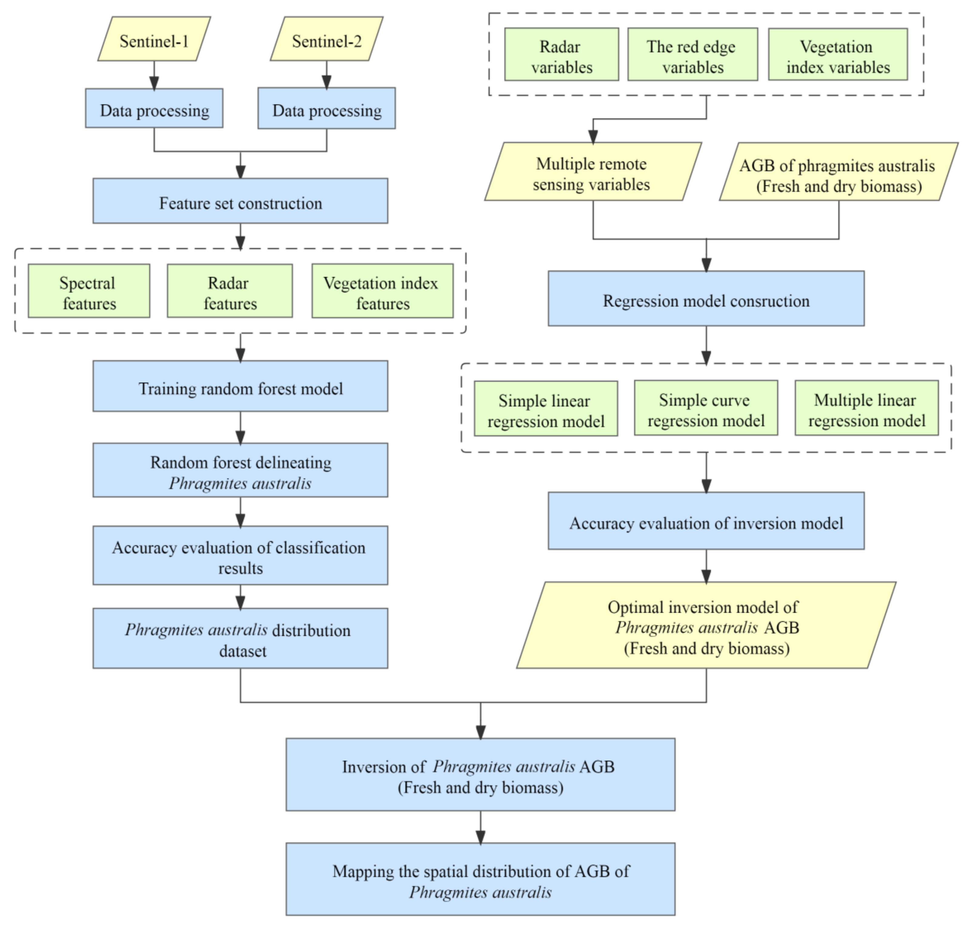
Three 1 × 1 m quadrats were randomly obtained from each sample plot (100 m × 100 m) with a sampling frame. P. australis vegetation in the study area is regularly harvested each year, so the biomass of the dried P. australis stems was not considered in this paper. All overground parts of P. australis plants in the quadrats were cut, and the environmental background (whether there was obvious human interference, etc.) of samples was recorded to eliminate other interference. The few P. australis that were in an unnatural growth state due to human trampling disturbances needed to be removed during sample processing. Preset sampling considers, as much as possible, the vegetative structure and environmental differences of the P. australis. The sampled P. australis ranged from 30 to 220 cm in height, with fully grown green stems that had not yet flowered. According to the distribution characteristics and growth density of P. australis in the study area, a total of 186 typical samples were selected for sampling. The samples were taken to the laboratory and weighed in fresh condition. The fresh AGB weight of each sample was obtained by averaging the fresh AGB weight of the three quadrats. The AGB for all samples were dried at 65 °C to constant weight, and the dry weight of AGB per unit area of P. australis was calculated by taking the mean value.

2.3. Methods

The distribution of P. australis was delineated by a random forest algorithm and the AGB of P. australis was spatially estimated by a regression model (Figure 2). First, the Sentinel-1 and Sentinel-2 images were preprocessed to construct a feature set of classification variables (Section 2.3.1). The random forest model was trained to classify land cover at the site and identify P. australis (Section 2.3.2). A variety of remote sensing variables were selected for correlation analysis (Section 2.3.3), and significantly correlated remote sensing variables with AGB of samples were selected to construct a regression linear model for AGB inversion (Section 2.3.4). Finally, the accuracy of delineating P. australis and the inversion model of AGB were evaluated (Section 2.3.5).

2.3.1. Classification System and Classification Feature Sets

Referring to the national atlas of land cover classification system [37] and considering the study focus, the land cover in the Momoge Ramsar site was categorized into vegetated wetland, water body (rivers, lakes, and artificial ponds), woodland, grassland, artificial vegetation, and barren land [38]. Vegetated wetland consists of multiple vegetation types, and we separated P. australis from other wetland vegetation.

Studies have shown that the integration of Sentinel-1 and Sentinel-2 can improve the accuracy of mapping land cover [39,40]. Two sensitive vegetation indices, the normalized difference vegetation index (NDVI) and the enhanced vegetation index (EVI), were selected based on Sentinel-2 data. The two radar features of Sentinel-1, VV and VH polarization backscattering coefficients, and 10 bands of Sentinel-2 (R, G, B, NIR, VRE1, VRE2, VRE3, NIR2, SWIR1, SWIR2) were used for the remote sensing vector feature set.

2.3.2. Training the Random Forest Model

Random forest is a common method in machine learning. It is an integration algorithm based on a decision tree, which uses multiple trees to train and predict samples. The bagging method is adopted in a random forest to generate an independent training sample set with the same distribution for each decision tree, and the final classification result depends on the votes of all decision trees [41,42]. The key to using random forest to measure the importance of features is to evaluate the contribution of each feature in each decision tree, calculate the average value, and then compare the contribution value of features [43].

The classification experiment in this study was based on the random forest module in ENVI. Based on this module, the bagging framework of random forest regression had the following parameters: the number of trees was 100 and the number of features was the square root method by default. The Gini Coefficient was selected for the impurity function and Min Node Sample was 1.

2.3.3. Selecting Remote Sensing Variables for Predicting P. australis AGB

As shown in the Table 1, VV and VH polarization backscattering coefficients were extracted from preprocessed Sentinel-1, and the 10 spectral bands were obtained from Sentinel-2. The three unique red-edge bands of Sentinel-2 were effective for monitoring vegetation, and B5, B6, and B7 were selected as remote sensing variables for AGB inversion. According to the characteristics of the study area and the relevant results of AGB remote sensing inversion at home and abroad [44,45,46], the difference vegetation index (DVI), enhanced vegetation index (EVI), normalized difference vegetation index (NDVI), inverted red edge chlorophyll index (IRECI), soil adjusted vegetation index (SAVI), modified soil-adjusted vegetation index (MSAVI), and the modified chlorophyll absorption ratio index (MCARI) were used to facilitate AGB estimation. The vegetation index was calculated using the Band Math tool. Since the data were raster structure, the vegetation index value of each sample was the corresponding pixel value on the vegetation index image. The description and calculation formula are shown in

Table 2. Remote sensing variables and calculation formulas.

Variable Types	Name of Remote Sensing Variables	Description or Calculation Formula
Radar characteristics	VV	VV polarization backscattering coefficient
	VH	VH polarization backscattering coefficient
Red edge band characteristics	B5 (VRE-1)	Sentinel-2 Vegetation Red Edge band 1
	B6 (VRE-2)	Sentinel-2 Vegetation Red Edge band 2
	B7 (VRE-3)	Sentinel-2 Vegetation Red Edge band 3
Vegetation index characteristics	DVI	NIR-Red
	EVI	2.5(NIR − Red)/(NIR + 6Red − 7.5Blue + 1)
	NDVI	(NIR − Red)/(NIR + Red)
	SAVI	((NIR − Red)/(NIR + Red + L))(1 + L)
	MSAVI	$\frac{2NIR+1-\sqrt{{\left(2NIR+1\right)}^2-8NIR-Red}}{2}$
	MCARI	((VRE1 − Red) − 0.2(VRE1 − Green))(VRE1/NIR)
	IRECI	(VRE3-Red)/(VRE1/VRE2)

. SPSS Statistics 22 was used to analyze the correlation between fresh and dry AGB weight of each remote sensing variable and P. australis sample, and the sensitivity of P. australis AGB to different remote sensing variables was calculated.

2.3.4. AGB Inversion Regression Model

Correlation coefficients were used to analyze remote sensing variables and vegetation AGB. Correlation analysis of 12 remote sensing variables with fresh and dry AGB weight of P. australis (177 samples) was conducted. Correlation analysis is a statistical method used to study the correlation between variables, and the magnitude of the correlation coefficient indicates the strength of correlation between the variables [47,48]. The formula is:

$$\mathrm{R}=\frac{\mathrm{n}{{\displaystyle \sum }}_{i=1}^n{x}_i{y}_i-{{\displaystyle \sum }}_{i=1}^n{x}_i·{{\displaystyle \sum }}_{i=1}^n{y}_i}{\sqrt{n{{\displaystyle \sum }}_{i=1}^n{x}_i^2-{\left({{\displaystyle \sum }}_{i=1}^n{x}_i\right)}^2}·\sqrt{n{{\displaystyle \sum }}_{i=1}^n{y}_i^2-{\left({{\displaystyle \sum }}_{i=1}^n{y}_i\right)}^2}}$$

(1)

where R is the correlation coefficient, x_i and y_i are the values of independent and dependent variables at various points, and n is the number of sample points.

A simple linear regression model has been widely used to estimate AGB, and to obtain a linear or nonlinear equation by regression fitting with a single vegetation index as an independent variable. The simple linear regression model is expressed as follows:

Y = β₀ + β₁x +u

(2)

the above expression represents the true relationship between variables Y and x, where Y is the dependent variable AGB, x is the independent remote sensing variable, u is the random error term, β₀ is the constant term, and β₁ is the regression coefficient. The above model can be divided into two parts: β₀ + β₁x is non-random and u is random.

Simple curve regression models are used to fit the curvilinear correlation between vegetation index and AGB, using an exponential model or high-order equation. Although the model fitting accuracy has been improved, due to the basis of the algorithm itself, there will be large errors in the inversion results for uneven areas of vegetation coverage. The polynomial equation is the basic model of AGB, and the formula is as follows:

Y = β₀ + β₁x₁ + β₂x₂ +…+ β_mx_m + u,

(3)

where Y is the dependent variable of vegetation AGB, x_i (i = 1, 2, …, m) is the independent remote sensing variable, βj (j = 1, 2, …, m) is the regression coefficient, and u is the residual error.

This multiple linear regression model was first defined to solve economic problems. In practical economic problems (and other fields such as geography and data statistics), a dependent variable is affected by multiple predictor variables [49]. The general form of the multiple linear regression model is:

Y = β₀ + β₁x₁ + β₂x₂ +…+ β_kx_i + u

(4)

where Y is the dependent variable vegetation AGB, x_i (i = 1, 2, …, n) is the independent remote sensing variable, k is the number of explanatory variables, βj (j = 1, 2, …, k) is the regression coefficient, and u is the error coefficient. The above formula is also known as the random expression of the population regression function.

Studies have shown that the AGB of vegetation in the growing state is correlated with various vegetation indices [50,51]. In AGB inversion model construction, it is more accurate and practical to estimate AGB by integrating multiple remote sensing variables and vegetation indexes, than by using only a single variable.

2.3.5. Precision Validation

Combined with the field P. australis samples and the verification samples selected visually on Google Earth, accuracy evaluation was conducted by combining visual evaluation and the confusion matrix. The obvious classification error targets were verified visually, and the confusion matrix was used to quantitatively evaluate the classification accuracy. Three indices including overall accuracy, Kappa coefficient, and mapping accuracy were selected.

For the inverse regression model, three indices, R², F, and P, were selected to evaluate the accuracy of the regression equation. R² was the coefficient of determination, and its value reflected the tightness of the sample data fitting the regression equation and the degree of prediction coincidence. R² is calculated by:

$${\mathrm{R}}^2=\frac{{{\displaystyle \sum }}_{i=1}^n{\left(\widehat{y^i}-\overline{y}\right)}^2}{{{\displaystyle \sum }}_{i=1}^n{\left(y^i-\overline{y}\right)}^2}$$

(5)

where $\widehat{y^i}$ is the model estimate of AGB, yⁱ is the measured value of AGB, $\overline{y}$ is the mean of the measured values of AGB, and n is the number of samples.

The F value is the result of variance analysis and is the overall test of the whole regression equation. P refers to the significance test of the regression equation. If the corresponding p-value is less than 0.05, the regression equation can be considered to be a significant predictor.

A scatter diagram was produced for the optimal regression model to verify the fitting effect of the model, and field data were selected from 21 P. australis sites sampled in the field. The field measured values were compared with the estimated values of the optimal regression model to verify the accuracy of the model through the relative error size.

3. Results

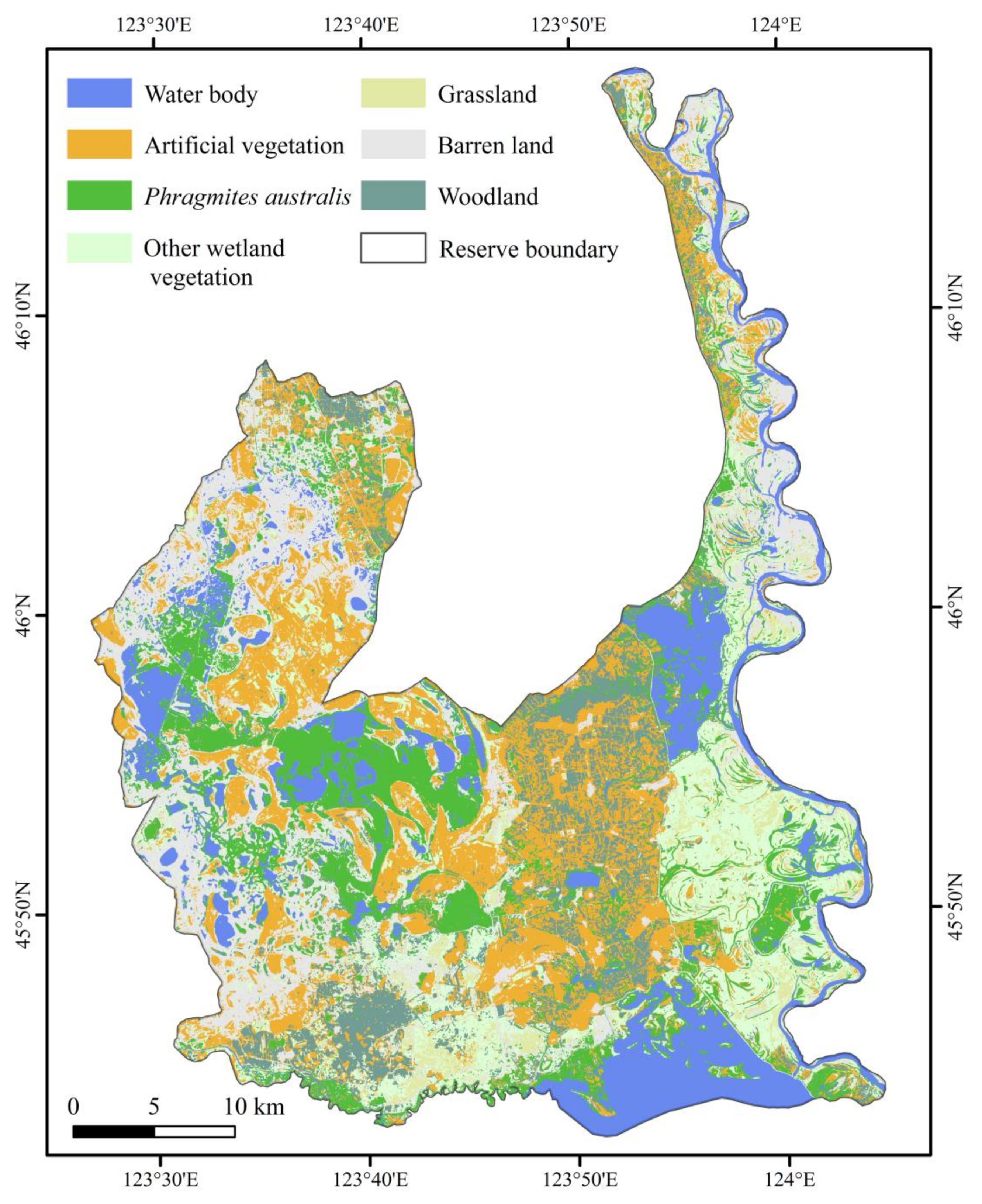
3.1. Classification Accuracy and Spatial Pattern of P. australis

Table 3. Confusion matrix of land cover classification in the Momoge Wetland Ramsar site.

	P. australis	Water Body	Barren Land	Wood Land	Grassland	Other Wetland Vegetation	Artificial Vegetation	Total
P. australis	4173	19	0	3	0	59	237	4491
Water body	13	11,808	0	0	0	0	0	11,821
Barren land	0	0	2900	0	25	0	216	3141
Woodland	26	0	0	2137	11	159	11	2344
Grassland	0	0	2	0	4409	436	12	4859
Other wetland vegetation	0	0	3	143	1396	3800	14	5436
Artificial vegetation	312	0	133	572	0	38	2169	3224
Total	4524	11,827	3038	2855	5841	4572	2659	35,316
Producer Accuracy%	92.24	99.84	95.46	74.85	75.48	84.86	81.57
User Accuracy%	92.92	99.89	92.36	91.17	90.76	71.39	67.28

Overall Accuracy = 89.13% Kappa Coefficient = 0.87.

presents the confusion matrix, overall accuracy (OA), and Kappa coefficients of the classification in this study, which revealed that random forest classification achieved good performance, with an overall accuracy of 89.13%, and Kappa coefficient of 0.87. The classification producer accuracy and user accuracy of P. australis vegetation were 92.24% and 92.92%, respectively.

The Momoge spatial distribution, consistent with the field survey results, is shown in Figure 3. There were fewer commission or omission errors, which indicated the effectiveness of the classification method.

P. australis was distributed widely in the middle and west parts of the study area. The distribution of P. australis was mostly concentrated in areas with abundant water, such as rivers and lakes. The total area of P. australis was 135.74 km², accounting for 9.1% of the entire Ramsar site.

3.2. Optimal Regression Model for Predicting P. australis AGB

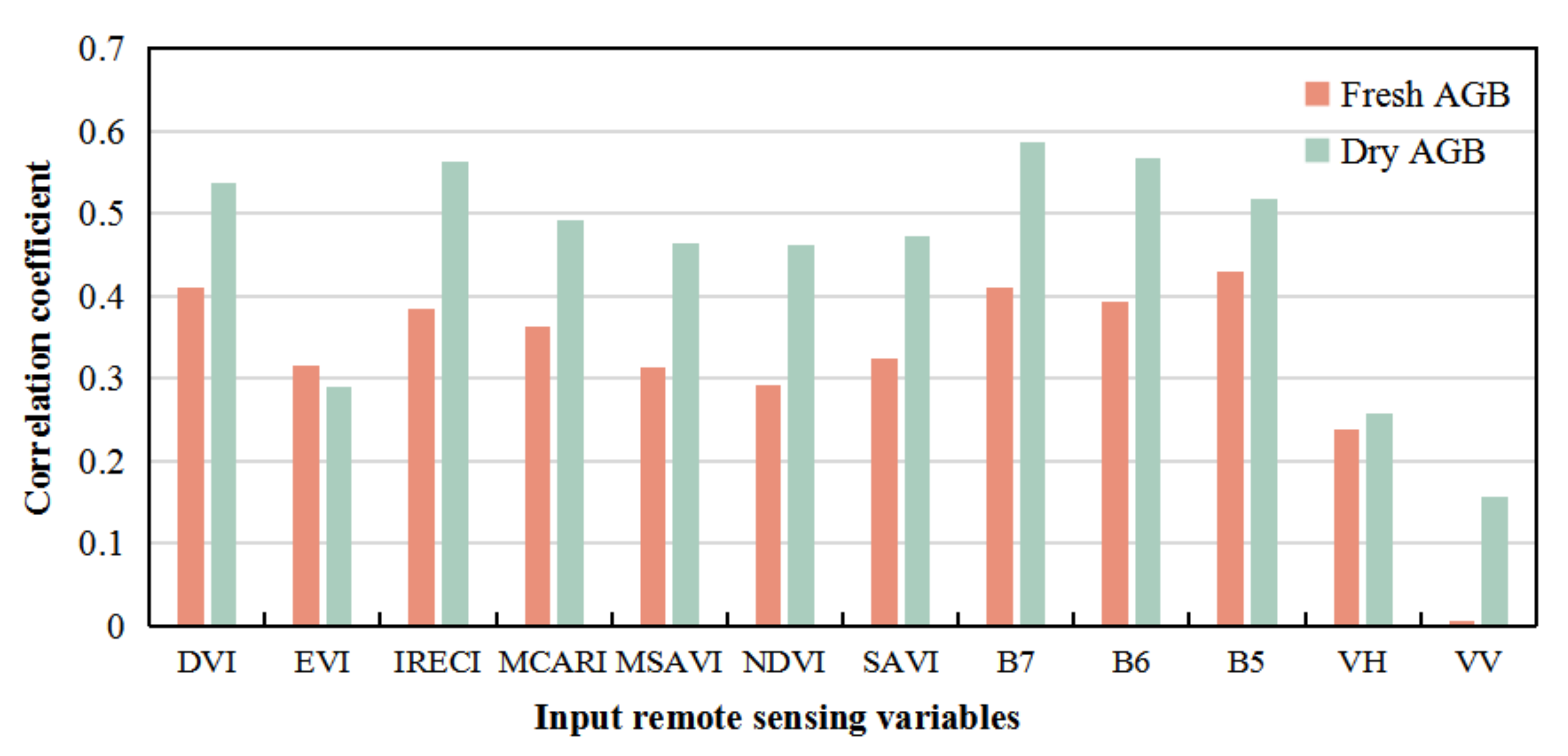
3.2.1. Sensitivity of Different Remote Sensing Variables to P. australis AGB

The samples of fresh and dry weight of P. australis AGB were tested for normal distribution, and of which nine samples with large deviations were removed. The correlation analysis between the remaining P. australis samples and the remote sensing variables showed that 11 remote sensing variables had a significant correlation with P. australis AGB at the p < 0.01 (significant correlations) level, except for the radar variable VV (Figure 4). The correlation coefficients between dry weight of P. australis AGB and DVI, IRECI, B7, B6, and B5 were all larger than 0.5, indicating that DVI, IRECI, B7, B6, and B5 were highly sensitive to the dry weight of AGB variance of P. australis. The sensitivity of the five remote sensing variables from large to small was B7 > B6 > IRECI > DVI > B5. The correlation coefficients between the fresh weight of P. australis AGB and DVI, B7 and B5 were all above 0.4, indicating that DVI, B7, and B5 were highly sensitive to the fresh weight of P. australis AGB, and the sensitivity of the three variables was B5 > DVI > B7. Through correlation analysis, remote sensing variables were selected to construct the remote sensing inversion model of P. australis dry and fresh weight of AGB.

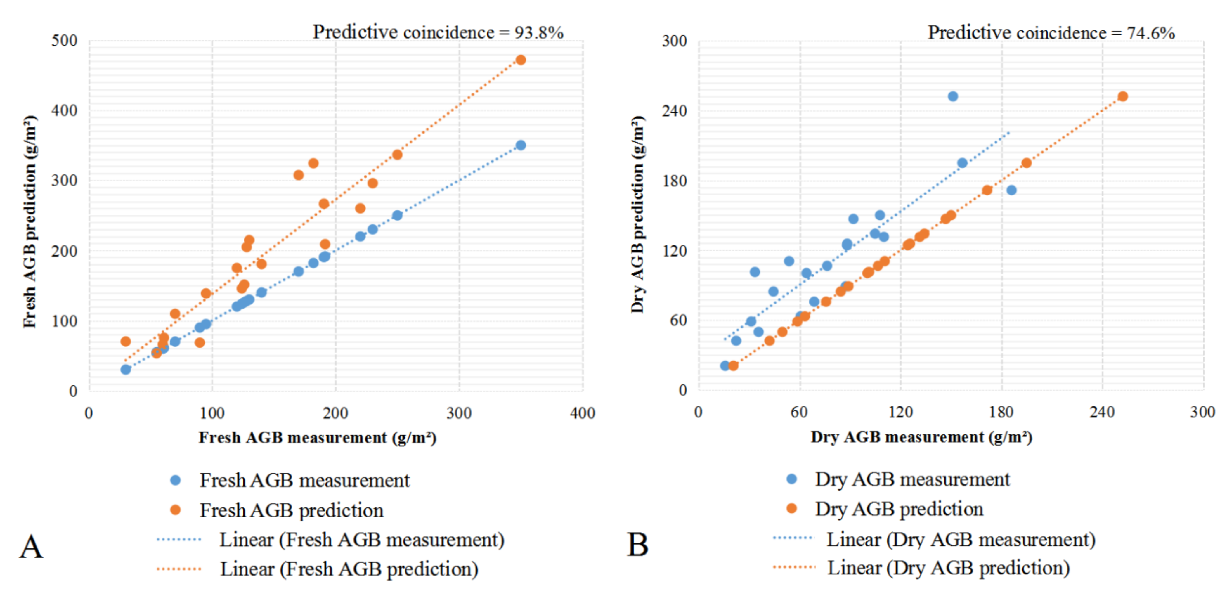
3.2.2. Optimal Regression Model and Accuracy Evaluation for Predicting P. australis AGB

A total of 11 remote sensing variables significantly correlating with dry and fresh weights of P. australis AGB were selected to construct the linear regressions (

Table A1. The simple linear regression models of AGB inversion.

	Simple Linear Regression Model		R2		F		P
	Fresh AGB	Dry AGB	Fresh AGB	Dry AGB	Fresh AGB	Dry AGB	Fresh AGB	Dry AGB
DVI	Y = 94.601X + 32.786	Y = 58.795X + 3.855	0.168	0.287	19.748	39.456	0.000	0.000
EVI	Y = −25474.1X + 12841.298	Y = -11140X + 5614.933	0.099	0.084	10.762	8.971	0.001	0.003
IRECI	Y = 988.958X + 48.703	Y = 688.448X + 11.128	0.148	0.317	16.960	45.440	0.000	0.000
MCARI	Y = −496.785X + 159.414	Y = -319.359X + 84.169	0.184	0.345	22.101	51.646	0.000	0.000
MSAVI	Y = 77.709X + 25.610	Y = 54.533X − 5.275	0.099	0.215	10.725	26.881	0.001	0.000
NDVI	Y = 62.920X + 45.448	Y = 47.494X + 6.611	0.084	0.213	9.033	26.534	0.003	0.000
SAVI	Y = 48.968X + 38.738	Y = 33.942X + 4.326	0.105	0.223	11.456	28.096	0.001	0.000
B7	Y = 92.998X + 35.745	Y = 63.534X + 2.731	0.167	0.241	19.631	31.084	0.000	0.000
B6	Y = 109.958X + 31.961	Y = 75.392X + 0.017	0.154	0.321	17.829	46.252	0.000	0.000
B5	Y = 583.525X − 46.448	Y = 334.526X − 39.109	0.132	0.268	14.938	35.877	0.000	0.000
VH		Y = 309.324X + 26.062		0.066		6.905		0.01

Y is AGB.

), simple curve regressions (

Table A2. The simple curve regression models of AGB inversion.

	Curve Regression Model	R2	F	P
	Fresh AGB	Fresh AGB	Fresh AGB	Fresh AGB
DVI	Y = 1013.351X − 2062.661X2 + 1434.618X3	0.192	7.603	0.000
IRECI	Y = 3060.607X − 86,367.302X2 + 999,864.866X3 + 37.16	0.403	43.44	0.000
MCARI	Y = −1385.306X + 2895.829X2 + 225.919	0.134	7.535	0.001
MSAVI	Y = 722.027X − 1308.796X2 + 805.478X3 − 66.292	0.115	4.174	0.008
NDVI	Y = 686.102X − 1525.248X2 + 1109.235X3 − 24.43	0.112	4.024	0.01
SAVI	Y = 412.465X − 599.9X2 + 293.628X3 − 21.856	0.125	4.592	0.005
B7	Y = 247.359X − 447.164X2 + 372.205X3 + 22.05	0.172	6.642	0.000
B6	Y = 250.181X − 490.966X2 + 478.936X3 + 22.842	0.158	6.016	0.001
B5	Y = 87.605X + 1134.670X2 + 7.059	0.185	11.016	0.000
	Curve Regression Model	R2	F	P
	Dry AGB	Dry AGB	Dry AGB	Dry AGB
DVI	Y = 454.874X − 815.043X2 + 525.493X3 − 55.01	0.301	13.788	0.000
IRECI	Y = 540.258X + 13,446.345X2 − 206,133.785X3 + 9.802	0.432	53.047	0.000
MCARI	Y = 170.852X − 1597.673X2 + 47.478	0.246	15.807	0.000
MSAVI	Y = 181.920X − 303.982X2 + 205.433X3 − 18.921	0.226	9.333	0.000
NDVI	Y = 290.012X − 590.474X2 + 427.825X3 − 20.792	0.231	9.598	0.000
SAVI	Y = 160.815X − 207.596X2 + 101.023X3 − 17.116	0.233	9.737	0.000
B7	Y = -99.743X + 423.332X2 − 328.471X3 + 20.538	0.355	17.621	0.000
B6	Y = −251.365X + 874.941X2 − 721.383X3 + 36.285	0.332	15.869	0.000
B5	Y = 1002.791X − 1528.997X2 − 111.212	0.277	18.54	0.000
VH	Y = 1831.173X − 30,031.630X2 + 146,088.610X3 + 5.927	0.1	3.566	0.017

Y is AGB.

), and multiple linear regression models. The comparison of model R² values showed that the optimal inversion models for fresh and dry weights of P. australis AGB were all multiple linear regression models, and the model formula is shown in

Table 4. Optimal regression model for AGB inversion.

	Multiple Linear Regression Model	R2	F	P
Fresh weight of AGB	Y = 856.114 + 379.777(B5) + 199.002(DVI) + 726.696(B7) − 785.183(B6) − 1514.958(IRECI) −208.821(MCARI) − 206.846(SAVI) − 1754.943(EVI) + 374.596(MSAVI) − 146.105(NDVI) −209.012(VH)	0.692	7.438	0.000
Dry weight of AGB	Y = −314.773 + 404.26(B7) − 446.934(B6) + 140.101(IRECI) + 29.898(DVI) + 212.375(B5) +106.868(MCARI) − 56.928(SAVI) + 88.964(MSAVI) − 16.539(NDVI) + 530.148(EVI) − 73.929(VH)	0.754	9.252	0.000

Y is AGB.

.

Table 4 shows that R² of the multiple regression models of fresh AGB weight and dry AGB weight were 0.692 and 0.754, respectively. To further evaluate the accuracy of the model, the field measurements were compared with the estimates from the multiple linear regression models. Scatter plots of relative errors were produced using field survey data and model prediction data (Figure 5). The dry AGB weight of predictive coincidence was 74.6%, fresh weight of AGB predictive coincidence was 93.8%, and the relative error between the estimated results and the measured data was mostly small. The relative error of samples near the pond was large because the pixels were not pure, which indicated that the calculation results of the model were consistent with the actual situation.

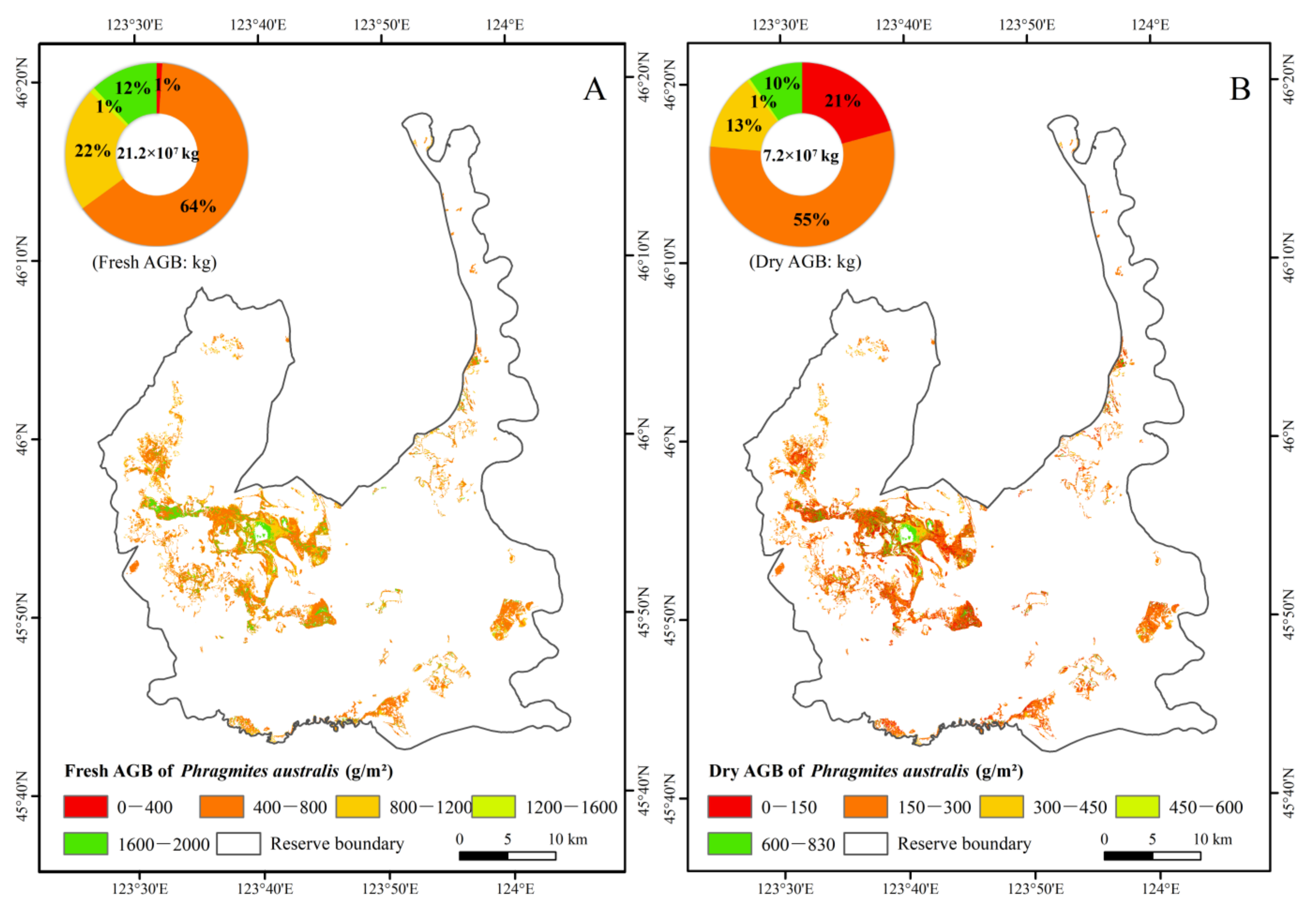
3.3. Spatial Estimates of P. australis AGB

The AGB of P. australis in the Ramsar site was estimated using the above optimal estimation models of fresh and dry weight of AGB. The maximum and minimum fresh weights of P. australis AGB in the region were 1926.05 g/m² and 20.12 g/m², and the maximum and minimum dry weights of P. australis AGB were 822.91 g/m² and 7.23 g/m², respectively. The average fresh and dry weights of AGB were 1566.03 g/m² and 531.86 g/m², respectively. The total fresh and dry weights of AGB of P. australis in the study area were 21.2 × 10⁷ kg and 7.2 × 10⁷ kg, respectively.

The fresh and dry weights of AGB were divided into five levels to obtain the spatial distribution map of the reserve AGB (Figure 6). Fresh weight of P. australis AGB primarily ranged 400–800 g/m², and dry weight of AGB 150–300 g/m². The higher AGB of P. australis was mainly found in the middle and west parts of the study area, while the high AGB of P. australis was concentrated around the rivers and lakes.

4. Discussion

We extracted P. australis distribution at the community scale from the Momoge Wetland Ramsar site using the random forest algorithm, combining the radar features of Sentinel-1 and the spectral characteristics of Sentinel-2. The classification accuracy was improved compared with a single type of remote sensing image [52,53], which has significant advantages in identifying the spatial distribution of wetland vegetation. In the random forest model, the three red-edge bands of Sentinel-2 and the two vegetation index features of NDVI and EVI were used to create variable feature ranks. The red-edge feature has capability to identify wetland vegetation [54,55]. Due to the instantaneous nature of surface information recorded by remote sensing images, there are often spatial differences in the same land types, resulting in misclassifications of “same matter with different spectrum” and “foreign matter with the same spectrum” [56,57]. In the future, we can try using multi-temporal remote sensing images to classify wetland vegetation in order to eliminate spatial differences.

Our results showed that the remote sensing variables with the highest correlation with AGB of P. australis were two Sentinel-2 red-edge bands (Figure 4). Red edge bands could indicate the sensitive spectrum of green plant growth conditions, which are less influenced by background information when used in vegetation identification [58,59]. Many previous studies have also shown that the use of Sentinel-2 red-edge band to construct vegetation index inversions can effectively predict vegetation growth characteristics [60,61]. Moreover, due to the high water content of P. australis in the fresh state, some spectral features have different limitations when used under the influence of water, resulting in a higher correlation between vegetation index and dry weight of AGB than that between vegetation index and fresh weight of P. australis AGB [62]. Our results also revealed that the accuracy of AGB inversion was improved by integrating Sentinel-1/2 red-edge indexes and radar features. When a traditional Thematic Mapper (TM) remote sensing image is used, the influence of water noise cannot be eliminated [63,64]. The level of vegetation information and different elements of vegetation can be obtained through different spectral channels of optical remote sensing [65]. However, when the penetration of optical remote sensing is insufficient, radar remote sensing can be used to obtain the canopy height of wetland vegetation [66]. Comparison with the results of related studies shows that the classification accuracy of combining the red-edge band of Sentinel-2 and radar scattering coefficients of Sentinel-1 in this paper was improved by 2–5% [67,68]. Therefore, the combination of Sentinel-1 and Sentinel-2 images is helpful to improve the accuracy of AGB inversion of P. australis vegetation.

The formation of P. australis as a single dominant species in perennially flooded areas leads to a higher AGB of P. australis. This is because wetland is under the condition of flooding, where soil organic matter and nitrogen elements are deposited, providing sufficient nutrients for plant growth and development [69,70]. In addition, abundant mineral nutrients in wetlands facilitate nutrient uptake and plant growth [71,72]. The spatial differences in P. australis growth are also affected by human activities, such as industrial effluents, road construction, and wasteland reclamation, with different disturbances from human activities in different regions [73]. The destruction of P. australis vegetation will affect the carbon sequestration function and ecological environment of wetland ecosystems [74]. P. australis not only can be used in papermaking and medicine, but also has strong economic and ecological values as the species can regulate climate and conserve water [75]. Therefore, the high-precision AGB inversion of P. australis can provide a reference for the restoration and management of P. australis. In order to further strengthen the conservation of P. australis resources in wetlands, the relevant departments should formulate wetland protection policies, raise the conservation awareness of residents, minimize the interference of human activities, effectively maintain the wetland functions and ecological environment, and achieve the scientific management and sustainable utilization of P. australis resources.

5. Conclusions

In this study, by combining Sentinel-1/2 satellite images, field-measured data, the random forest algorithm, and multiple regression models, we delineated the spatial distribution of P. australis in the Momoge Ramsar Wetland site and estimated the fresh and dry weight of P. australis AGB. The results showed that the overall accuracy of P. australis delineation based on Sentinel-1/2 images and the random forest method was 89.13%, and the producer accuracy of P. australis was 92.24%. The optimal inversion model of dry and fresh weight of AGB was the multiple linear regression model, and the predictive coincidence was 74.6% and 93.8%, respectively. In addition, the AGB of P. australis in the wetland was estimated by the model, and the fresh and dry weights of AGB were 21.2 × 10⁷ kg and 7.2 × 10⁷ kg in 2020. The distribution of P. australis AGB showed obvious spatial differences, and the high values were distributed mainly in the middle and west parts of the study area. The P. australis AGB pattern was successfully predicted by the proposed method with good accuracy, indicating the effectiveness of the Sentinel-1/2 data. In future studies at larger scales, different vegetative structures and environmental differences should be taken into account when obtaining ground samples as a way to ensure the generalizability of the model. The methods and generated data could benefit the sustainable management of the Momoge Wetland Ramsar site.

References

1. Mitsch, W.J.; Gosselink, J.G. Wetlands; John Wiley & Sons Inc.: New York, NY, USA, 1986. [Google Scholar]
2. Mitsch, W.J.; Gosselink, J.G. Wetlands, 2nd ed.; Van Nostrand Reinhold: New York, NY, USA, 1993. [Google Scholar]
3. Duman, T.; Schäfer, K.V.R. Partitioning net ecosystem carbon exchange of native and invasive plant communities by vegetation cover in an urban tidal wetland in the New Jersey Meadowlands (USA). Ecol. Eng. 2018, 114, 16–24. [Google Scholar] [CrossRef]
4. Mitsch, W.J.; Gosselink, J.G. Wetlands, 3rd ed.; John Wiley & Son, Inc.: New York, NY, USA, 2000. [Google Scholar]
5. Guo, N.; Liu, J. Overview of plant biomass research. Subtrop. Plant Sci. 2011, 40, 83–88. [Google Scholar]
6. Mao, D.; Luo, L.; Wang, Z.; Wilson, M.C.; Zeng, Y.; Wu, B.; Wu, J. Conversions between natural wetlands and farmland in China: A multiscale geospatial analysis. Sci. Total Environ. 2018, 634, 550–560. [Google Scholar] [CrossRef] [PubMed]
7. Wang, S.; Li, X.; Zhou, Y. Progress in estimating methods of wetland vegetation biomass. Geogr. Geo-Inf. Sci. 2004, 5, 104–109, 113. [Google Scholar]
8. Shao, C.; Chen, Z.; Dong, H. Study on the growth and biomass of Phragmites communis in liaohe Estuarine wetland. J. Liaoning Univ. (Nat. Sci. Ed.) 1995, 1, 89–94. [Google Scholar]
9. Liu, L.; Han, M.; Liu, Y. Spatial distribution of wetland vegetation biomass and its influencing factors in the Yellow River Delta Nature Reserve. Acta Ecol. Sin. 2017, 37, 4346–4355. [Google Scholar]
10. Wang, J.; Mao, D.; Du, H. Study on forest and swamp mapping of Hani Wetland using Sentinel 1/2 satellite imagery. Wetl. Sci. Manag. 2021, 17, 2–7+12. [Google Scholar]
11. Gaurav, K.; Kiran, K.S. Mapping and Monitoring the Selected Wetlands of Punjab, India, Using Geospatial Techniques. J. Indian Soc. Remote Sens. 2020, 48, 615–625. [Google Scholar]
12. Adam, E.; Mutanga, O.; Rugege, D. Multispectral and hyperspectral remote sensing for identification and mapping of wetland vegetation: A review. Wetl. Ecol. Manag. 2010, 18, 281–296. [Google Scholar] [CrossRef]
13. Mutanga, O.; Adam, E.; Cho, A. High density biomass estimation for wetland vegetation using WorldView-2 imagery and random forest regression algorithm. Int. J. Appl. Earth Obs. Geoinf. 2012, 18, 399–406. [Google Scholar] [CrossRef]
14. Jensen, D.; Cavanaugh, K.; Simard, M.; Christensen, A.; Rovai, A. Aboveground biomass distributions and vegetation composition changes in Louisiana’s Wax Lake Delta. Estuar. Coast. Shelf Sci. 2021, 250, 107–139. [Google Scholar] [CrossRef]
15. Yang, Q.; Yuan, Q.; Li, T. Mapping PM 2.5 concentration at high resolution using a cascade random forest based downscaling model: Evaluation and application. J. Clean. Prod. 2020, 277, 1–12. [Google Scholar] [CrossRef]
16. Gou, F.; Zhao, C.; Yang, J. Spatial pattern of aboveground biomass and its response to water and salinity in sugan Lake wetland. Acta Ecol. Sin. 2021, 19, 1–11. [Google Scholar]
17. Yu, H.; Wu, Y.; Jin, Y. Retrieval of aboveground biomass from MODIS SWIR data and its spatio-temporal variation in arid region. Remote Sens. Technol. Appl. 2017, 32, 524–530. [Google Scholar]
18. Dinh, H.T.M. Potential value of combining ALOS PALSAR and Landsat-derived tree cover data for forest biomass retrieval in Madagascar. Remote Sens. Environ. 2018, 213, 206–214. [Google Scholar]
19. Ramon, T.; Paul, S.; Dirk, G. GMES Sentinel- 1 mission. Remote Sens. Environ. 2012, 120, 9–24. [Google Scholar]
20. Su, W.; Hou, N.; Li, Q. Retrieval of leaf area index of maize canopy based on Sentinel-2 remote sensing images. Trans. Chin. Soc. Agric. Mach. 2018, 49, 151–156. [Google Scholar]
21. Oliver, C.; Maurizio, S. Exploring combinations of multi-temporal and multi-frequency radar backscatter observations to estimate above-ground biomass of tropical forest. Remote Sens. Environ. 2019, 232, 111313. [Google Scholar]
22. Oliver, S.; Andrea, N.; Osama, Y. Dimensionality Reduction and Feature Selection for Object-Based Land Cover Classification based on Sentinel-1 and Sentinel-2 Time Series Using Google Earth Engine. Remote Sens. 2019, 12, 76. [Google Scholar]
23. Jelének, J.; Kopačková-Strnadová, V. Synergic use of Sentinel-1 and Sentinel-2 data for automatic detection of earthquake-triggered landscape changes: A case study of the 2016 Kaikoura earthquake (Mw 7.8), New Zealand. Remote Sens. Environ. 2021, 265. [Google Scholar] [CrossRef]
24. Investigators at Free University of Bozen-Bolzano Report Findings in Remote Sensing. Exploiting Time Series of Sentinel-1 and Sentinel-2 Imagery To Detect Meadow Phenology In Mountain Regions. Remote Sensing. 2019, 11, 542. [Google Scholar] [CrossRef] [Green Version]
25. Li, Y.; Zhang, C.; Heng, W. Retrieving Surface Soil Moisture over Wheat-Covered Areas Using Data from Sentinel-1 and Sentinel-2. Water 2021, 13, 1981. [Google Scholar] [CrossRef]
26. Wang, H.; Zhang, X.; Wu, W. Prediction of Soil Organic Carbon under Different Land Use Types Using Sentinel-1/-2 Data in a Small Watershed. Remote Sens. 2021, 13, 1229. [Google Scholar] [CrossRef]
27. Xing, X.; Yang, X.; Xu, B. Estimation of aboveground biomass using remote sensing based on random forest algorithm. J. Geo-Inf. Sci. 2021, 23, 1312–1324. [Google Scholar]
28. O’Shea, R.E. Advancing cyanobacteria biomass estimation from hyperspectral observations: Demonstrations with HICO and PRISMA imagery. Remote Sens. Environ. 2021, 266, 112693. [Google Scholar] [CrossRef]
29. Tewes, A. Assimilation of Sentinel-2 Estimated LAI into a Crop Model: Influence of Timing and Frequency of Acquisitions on Simulation of Water Stress and Biomass Production of Winter Wheat. Agronomy 2020, 10, 1813. [Google Scholar] [CrossRef]
30. Yuan, Y.; Yuan, L.; Sheng, H. Influence of Spectral Bandwidth and Position on Chlorophyll Content Retrieval at Leaf and Canopy Levels. J. Indian Soc. Remote Sens. 2016, 44, 583–593. [Google Scholar]
31. Schmid, T.; Koch, M.; Gumuzzio, J.; Mather, P.M. A spectral library for a semi-arid wetland and its application to studies of wetland degradation using hyperspectral and multispectral data. Int. J. Remote Sens. 2004, 25, 2485–2496. [Google Scholar] [CrossRef]
32. Li, C.; Zhou, L.; Xu, W. Estimating Aboveground Biomass Using Sentinel-2 MSI Data and Ensemble Algorithms for Grassland in the Shengjin Lake Wetland, China. Remote Sens. 2021, 13, 1595. [Google Scholar] [CrossRef]
33. The Secretariat of the Convention on Wetlands. The List of Wetlands of International Importance. 2020. Available online: https://www.ramsar.org/sites/default/files/documents/library/sitelist.pdf (accessed on 15 October 2021).
34. Jiang, H.; He, C.; Luo, W. Hydrological restoration and water resource management of siberian crane (Grus leucogeranus) stopover wetlands. Water 2018, 10, 1714. [Google Scholar] [CrossRef] [Green Version]
35. Liu, C.; Zuo, Y.; Ren, B. Study on insect diversity in momoge national nature reserve. J. Northeast. Norm. Univ. (Nat. Sci.) 2011, 43, 112–116. [Google Scholar]
36. Li, S.; An, Y.; Wang, X. Species composition and quantitative characteristics of plant communities in Momoge Wetland under different surface water levels. Wetl. Sci. 2015, 13, 466–471. [Google Scholar]
37. Wu, B.; Qian, J.; Zeng, Y. Land Cover Atlas of the People’s Republic of China (1:10 Million); China Cartographic Publishing House: Beijing, China, 2017. [Google Scholar]
38. Yan, H.; Zhu, W.; Mao, D. Remote sensing analysis of anthropogenic stress in internationally important wetlands of Yangtze river delta. China Environ. Sci. 2020, 40, 3605–3615. [Google Scholar]
39. Hu, B.; Xu, Y.; Huang, X. Improving Urban Land Cover Classification with Combined Use of Sentinel-2 and Sentinel-1 Imagery. ISPRS Int. J. Geo-Inf. 2021, 10, 533. [Google Scholar] [CrossRef]
40. Ghorbanian, A.; Zaghian, S.; Asiyabi, R.M. Mangrove Ecosystem Mapping Using Sentinel-1 and Sentinel-2 Satellite Images and Random Forest Algorithm in Google Earth Engine. Remote Sens. 2021, 13, 2565. [Google Scholar] [CrossRef]
41. Guo, X.; Zhang, C.; Luo, W. Urban impervious surface extraction based on multi-features and random forest. IEEE Access 2020, 8, 226609–226623. [Google Scholar] [CrossRef]
42. Yao, M. Random Forests and Its Application to the Classification of Remote Sensing Image; Huaqiao University: Quanzhou, China, 2014. [Google Scholar]
43. Breiman, L. Random forests. Mach. Learn. 2001, 45, 5–32. [Google Scholar] [CrossRef] [Green Version]
44. Lu, D.; Chen, Q.; Wang, G. A survey of remote sensing-based aboveground biomass estimation methods in forest ecosystems. Int. J. Digit. Earth 2014, 13, 1–43. [Google Scholar] [CrossRef]
45. Zhang, G.; Ganguly, S.; Nemani, R.R. Estimation of forest aboveground biomass in California using canopy height and leaf area index estimated from satellite data. Remote Sens. Environ. 2014, 151, 44–56. [Google Scholar] [CrossRef]
46. Mao, D.; Wang, Z.; Li, L. Spatiotemporal dynamics of grassland aboveground net primary productivity and its association with climatic pattern and changes in Northern China. Ecol. Indic. 2014, 41, 40–48. [Google Scholar] [CrossRef]
47. Yang, C.; Liu, J.; Huang, H. Correlation analysis between tropical forest vegetation biomass and remote sensing geo-data. Geogr. Res. 2005, 24, 473–479. [Google Scholar]
48. Zhang, J.; Pan, G. Comparison and application of multiple linear regression and BP neural network prediction model. J. Kunming Univ. Technol. Nat. Sci. Ed. 2013, 38, 61–67. [Google Scholar]
49. Li, J.; Shu, X.; Chen, S. Remote sensing monitoring model of poyang Lake wetland vegetation biomass based on LandSAT-TM data. J. Guangzhou Univ. (Nat. Sci. Ed.) 2005, 6, 494–498. [Google Scholar]
50. Xu, J. Mathematical Methods in Modern Geography; Higher Education Press: Beijing, China, 2002; pp. 47–60. [Google Scholar]
51. Li, X.; Yeh, A.; Liu, K. Inventory of mangrove wetlands in the pearl river estuary of China using remote sensing. J. Geogr. Sci. 2006, 16, 155–164. [Google Scholar] [CrossRef]
52. Lei, X.; Yang, B.; Jiang, W. Changes of vegetation pattern and its influencing factors in east dongting wetland. Geogr. Res. 2012, 31, 461–470. [Google Scholar]
53. Xiang, D.; Wu, Y.; Zhang, R. Classification of coastal wetland vegetation using remote sensing. Shanxi Meteorol. 2011, 2, 19–24. [Google Scholar]
54. Shan, J.; Fang, W.; Lu, M. Local detrended fluctuation analysis for spectral red-edge parameters extraction. Nonlinear Dyn. 2018, 93, 995–1008. [Google Scholar]
55. Yumiko, K.; Brenda, T.; Marilyn, D. Evaluation of red and red-edge reflectance-based vegetation indices for rice biomass and grain yield prediction models in paddy fields. Precis. Agric. 2016, 17, 507–530. [Google Scholar]
56. Mountrakis, G.; Im, J.; Ogole, C. Support vector machines in remote sensing: A review. ISPRS J. Photogramm. Remote Sens. 2011, 66, 247–259. [Google Scholar] [CrossRef]
57. Melgani, F.; Bruzzone, L. Classification of hyperspectral remote sensing images with support vector machines. IEEE Trans. Geosci. Remote Sens. 2004, 42, 1778–1790. [Google Scholar] [CrossRef] [Green Version]
58. Filella, I.; Penuelas, J. The red edge position and shape as indicators of plant chlorophyll content, biomass and hydric status. Int. J. Remote Sens. 1994, 15, 1459–1470. [Google Scholar] [CrossRef]
59. Hansen, P.; Schjoerring, J. Reflectance measurement of canopy biomass and nitrogen status in wheat crops using normalized difference vegetation indices and partial least squares regression. Remote Sens. Environ. 2003, 86, 542–553. [Google Scholar] [CrossRef]
60. Song, K.; Zhang, B.; Li, F. Correlation analysis of hyperspectral reflectance with soybean leaf area and aboveground fresh biomass. Trans. Chin. Soc. Agric. Eng. 2005, 21, 36–40. [Google Scholar]
61. Frampton, W.; Dash, J.; Watmough, G. Evaluating the capabilities of Sentinel-2 for quantitative estimation of biophysical variables in vegetation. ISPRS J. Photogramm. Remote Sens. 2013, 82, 83–92. [Google Scholar] [CrossRef] [Green Version]
62. Li, S.; Li, X.; Ying, G. Biomass model of typical steppe region based on VEGETATION index: A case study of Xilinhot City, Inner Mongolia. Chin. J. Plant Ecol. 2007, 31, 23–31. [Google Scholar]
63. Zhang, M.; Ustin, S.; Rejmankova, E. Monitoring Pacific coast salt marshes using remote sensing. Ecol. Appl. 1997, 7, 1039–1053. [Google Scholar] [CrossRef]
64. Shi, Z.; Ma, Y.; Wang, Y. Advances in land use/cover classification using remote sensing images. Chin. Agric. Sci. Bull. 2012, 28, 273–278. [Google Scholar]
65. Swatantran, A.; Dubayah, R.; Roberts, D. Mapping biomass and stress in the Sierra Nevada using lidar and hyperspectral data fusion. Remote Sens. Environ. 2011, 115, 2917–2930. [Google Scholar] [CrossRef] [Green Version]
66. Megan, W.; Lang, E.; Kasischke, S.; Prince, S.D.; Pittman, K.W. Assessment of C-band synthetic aperture radar data for mapping and monitoring Coastal Plain forested wetlands in the Mid-Atlantic Region, U.S.A. Remote Sens. Environ. 2007, 112, 4120–4130. [Google Scholar]
67. Wang, G.S.; Wang, N.; Guo, W.L. Modelling Forest Aboveground Biomass Based on GF-3 Dual-Polarized and WorldView-3 Data: A Case Study in Datong National Wetland Park, China. Math. Probl. Eng. 2021, 2021, 9925940. [Google Scholar] [CrossRef]
68. Bucha, T.; Papčo, J.; Sačkov, I.; Pajtík, J. Woody Above-Ground Biomass Estimation on Abandoned Agriculture Land Using Sentinel-1 and Sentinel-2 Data. Remote Sens. 2021, 13, 2488. [Google Scholar] [CrossRef]
69. Ren, L.; Wang, M.; Li, C. Impacts of human activities on river runoff in the northern area of China. J. Hydrol. 2002, 261, 204–217. [Google Scholar] [CrossRef]
70. Xu, Z.; He, Y.; Yan, B.; Ren, H. Effects of nutrient and water level changes on wetland plants. Chin. J. Ecol. 2006, 25, 87–92. [Google Scholar]
71. Lawson, T.; Vialet-Chabrand, S. Speedy stomata, photosynthesis and plant water use efficiency. New Phytol. 2019, 221, 93–98. [Google Scholar] [CrossRef] [PubMed] [Green Version]
72. Gorai, M.; Laajili, W.; Santiago, L. Rapid recovery of photosynthesis and water relations following soil drying and rewatering is related to the adaptation of desert shrub Ephedra alata subsp. alenda (Ephedraceae) to arid environments. Environ. Exp. Bot. 2015, 109, 113–121. [Google Scholar] [CrossRef] [Green Version]
73. Zhang, M.; Wang, X.; Tong, S. Study on plant community species diversity in momoge Wetland restoration area. Wetl. Sci. 2021, 19, 458–464. [Google Scholar]
74. Sun, X.; Chen, Y.; Zhuo, N.; Cui, Y. Effects of salinity and concomitant species on growth of Phragmites australis populations at different levels of genetic diversity. Sci. Total Environ. 2021, 780, 146516. [Google Scholar] [CrossRef]
75. Zhang, Y.; Yu, W.; Ji, R.; Zhao, Y.; Feng, R. Dynamic Response of Phragmites australis and Suaeda salsa to Climate Change in the Liaohe Delta Wetland. J. Meteorol. Res. 2021, 35, 157–171. [Google Scholar] [CrossRef]
Figure 1. The geographic location and sample location of the study area. The background image is from Sentinel-2.
Remotesensing 14 00694 g001
Figure 2. Flowchart of AGB inversion of Phragmites australis at the Momoge Ramsar site.
Remotesensing 14 00694 g002
Figure 3. Spatial distribution of land cover types in the Momoge Wetland Ramsar site.
Remotesensing 14 00694 g003
Figure 4. Correlation coefficients between remote sensing variables and AGB of Phragmites australis.
Remotesensing 14 00694 g004
Figure 5. Accuracy verification of the scatter diagram. (A) Fresh weight of AGB. (B) Dry weight of AGB.
Remotesensing 14 00694 g005
Figure 6. AGB pattern and statistics of Phragmites australis. (A) Fresh weight of AGB. (B) Dry weight of AGB.
Remotesensing 14 00694 g006