Article

Automatic Identification of Forest Disturbance Drivers Based on Their Geometric Pattern in Atlantic Forests

1
Forestry Engineering School, University of Vigo—A Xunqueira Campus, 36005 Pontevedra, Spain
2
CINTECX, GESSMin Group (Safe and Sustainable Management of Mineral Resources), 36310 Vigo, Spain
*
Author to whom correspondence should be addressed.
Remote Sens. 2022, 14(3), 697; https://doi.org/10.3390/rs14030697
Submission received: 20 December 2021 / Revised: 23 January 2022 / Accepted: 26 January 2022 / Published: 1 February 2022

Abstract

:
Monitoring forest disturbances has become essential towards the design and tracking of sustainable forest management. Multiple methodologies have been developed to detect these disturbances. However, few studies have focused on the automatic detection of disturbance drivers, an essential task as each disturbance has different implications for the functioning of the ecosystem and associated management actions. Wildfires and harvesting are two of the major drivers of forest disturbances across different ecosystems. In this study, an automated methodology is presented to automatically distinguish between the two once the disturbance is detected, using the properties of its geometry and shape. A cluster analysis was performed to automatically individualize each disturbance and afterwards calculate its geometric properties. Using these properties, a decision tree was built that allowed for the distinction between wildfires and harvesting with an overall accuracy of 91%. This methodology and further research relating to it could pose an essential aid to national and international agencies for incorporating forest-disturbance-driver-related information into forest-focused reports.

Graphical Abstract

1. Introduction

Forests play an essential role in modern societies since they provide valuable resources and ecosystem services, such as carbon and biodiversity reservoirs [1,2,3]. However, nowadays forests are threatened by anthropogenic pressures and climate change [1,4]. In this context, monitoring forests and their disturbances has become essential for developing management strategies oriented towards increasing forests’ resilience and guaranteeing their sustainability [5,6]. Since the signing of the Paris Agreement [7], which mandated the reporting of forest changes, carbon emissions and uptakes, a special need has arisen among national and international agencies to conduct forest disturbances detection, identification and quantification.
Wildfires have been identified as one of the major drivers of forest disturbances across many different ecosystems. According to the Global Forest Goals Report 2021, fire has been a prevalent forest disturbance in the tropics [8], as well as in boreal and temperate forest ecosystems [9,10]. However, nowadays the fire regimes in the forested ecosystems of Europe are currently gaining great relevance due to climate change [11]. In fact, climate driven wildfires have been highlighted by many countries as a significant threat compromising forest-based economic, social and environmental benefits [8]. Therefore, monitoring wildfires is a key point in forest change reporting.
Another relevant forest disturbance is forest harvesting. Worldwide national and international forest agencies put great effort into minimizing illegal logging in order to reduce the degradation of forest ecosystems [12,13]. However, it is also important for management agents to monitor legal forest harvesting in order to design sustainable management policies and evaluate progress towards a sustainable bio-economy. The monitoring of forest harvestings is also needed to ensure the traceability of forest products and to fulfill the European regulations related to legal wood supply [14]. Such forest monitoring becomes essential in countries or regions whose forests are mostly privately owned and with a very active forest sector. In these kind of areas, traditional forest harvesting monitoring based on field visits may not be feasible or fully efficient.
In this context, the open access to satellite data has marked a turning point in forest monitoring and disturbance detection [15]. Satellites, such as the family of Landsats and Sentinel-2, have been widely used to report forest extent and forest changes [15]. In the field of change detection, a wide range of methodologies and algorithms have been developed that are currently well established and widely used. The most efficient ones rely on time series analysis [16]. Some examples are the family of Breaks For Additive Season and Trend (BFAST) algorithms [17,18,19], LandTrender [20] and Continuous Change Detection and Classification (CCDC) [21]. As a result of the application of these kinds of algorithms, the location and extent of the disturbances can be automatically obtained, as well as the timing and degree of the disturbance.
However, proper forest monitoring requires more than the location and extent of disturbances. It would also be essential to automatically identify the drivers of the detected disturbances since each type of driver (i.e., harvesting, wildfires, windstorms or insect plagues) has different implications for forest management agents [22,23,24]. Forest agencies have traditionally derived this information from pre-existing databases [25,26,27,28], visual interpretation of very high-resolution images (VHR-imagery) [29] or even field work. The main drawbacks of these kind of approaches are that they can be outdated, time-consuming and/or expensive. Again, remote sensing constitutes an alternative for automating the identification of drivers in forest disturbances through efficient affordable procedures. In this field, spectral indexes have showed to be efficient in the detection of wildfires (as for example the NBR [30]), but they do not allow to differentiate wildfires from harvestings (the latter are usually detected as wildfires) [31,32]. Consequently, new approaches are needed.
Some interesting advances have been recently achieved in the identification of drivers of forest disturbances. In the context of disturbances in the USA, an algorithm has been developed that correlates each type of disturbance with the “shape” of the spectral response of the disturbance area over time [33]. This technique has been enhanced by including additional predictor variables that again rely on information, such as pre-existing fire-burn perimeters from pre-existing databases [34]. This enables the prediction of the disturbance causality on a large scale in US forests. A different study performed in boreal forests found that studying the spectral response of the short-wave infrared (SWIR) portion of the electromagnetic spectrum of the soil left behind after a disturbance provides an effective way of discriminating between harvesting and wildfires [35]. Supervised classification of different spectral metrics together with geometric metrics of changes has been used as well by Hermosilla et al. [36]. However, it is worth noting that Neigh et al. found difficulties when transferring between different ecosystems’ methods that rely on spectral response to detect disturbance drivers [37]. This can severely affect the application of such methods on very large scales [37]. Therefore, it may be valuable to analyze a different approach that is less dependent on the radiometric responses of the disturbances.
This study presents a novel methodology based on Sentinel-2 data to automatically identify the driver of forest disturbances, once they have been detected. Since previous studies make the point that forest disturbances such as wildfires and harvestings manifest different shapes [35,38,39], the proposed methodology uses the geometric and shape properties of the disturbances to identify the potential driver. It is applied to Galicia (Northwest of Spain), a region characterized by numerous and intense forest harvestings, frequent wildfires and a very high rate of private forests owners (99% of Galician forests are privately owned) [40,41]. Section two describes the study area, materials and methodology. Section three presents the obtained results. Section four accomplishes the discussion. Section five comes to the conclusions of the described methodology and its implementation to the selected study area.

2. Materials and Methods

2.1. Study Area

The present study was carried out in Galicia, a region in the Northwest of Spain (see Figure 1). This region encompasses a total of 29,574 km2, nearly 70% of which is covered by forest land [40]. Forest area is mainly covered by Pinus sp., Eucalyptus sp. and mixed broadleaves (riparian species, Quercus robur, Quercus pyrenaica and Castanea sativa, among others) [40,42]. Shrubs are abundant as well, comprising approximately 30% of the forest land cover [40,42].
The main forest disturbances in Galicia are due to wildfires and harvestings. In relation to wildfires, it might be highlighted that although Galicia represents only 6% of the Spanish land surface, between 2006 and 2015 it reported the largest number of wildfire events in Spain (it reported 29.22% of all Spanish wildfire events occurring between these two years) and accounted for the largest percentage of burned surface (22.51% of the total Spanish burned surface in these years) [43]. These trends have continued throughout subsequent years [44].
In relation to harvestings, it should be noted that Galicia has an active forestry sector [40,41,45,46]. More than half of the annual fellings in Spain are harvested in Galicia [45], making this area one of the European regions with the highest percentage of harvesting intensity [46]. Most forest harvesting actions are produced on private forests since 99% of Galician forests are privately owned [41]. Management actions are rarely uniform across the region as land property is highly fragmented; approximately 40% of the land covered by the main productive tree species in Galicia are in cadastral parcels smaller than 0.5 ha [47]. The mean of forest harvesting processed records per year in the last six years (2015–2020) amounts to 88,140 [41].

2.2. Satellite Image Acquisition
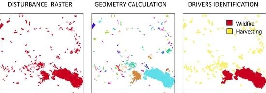
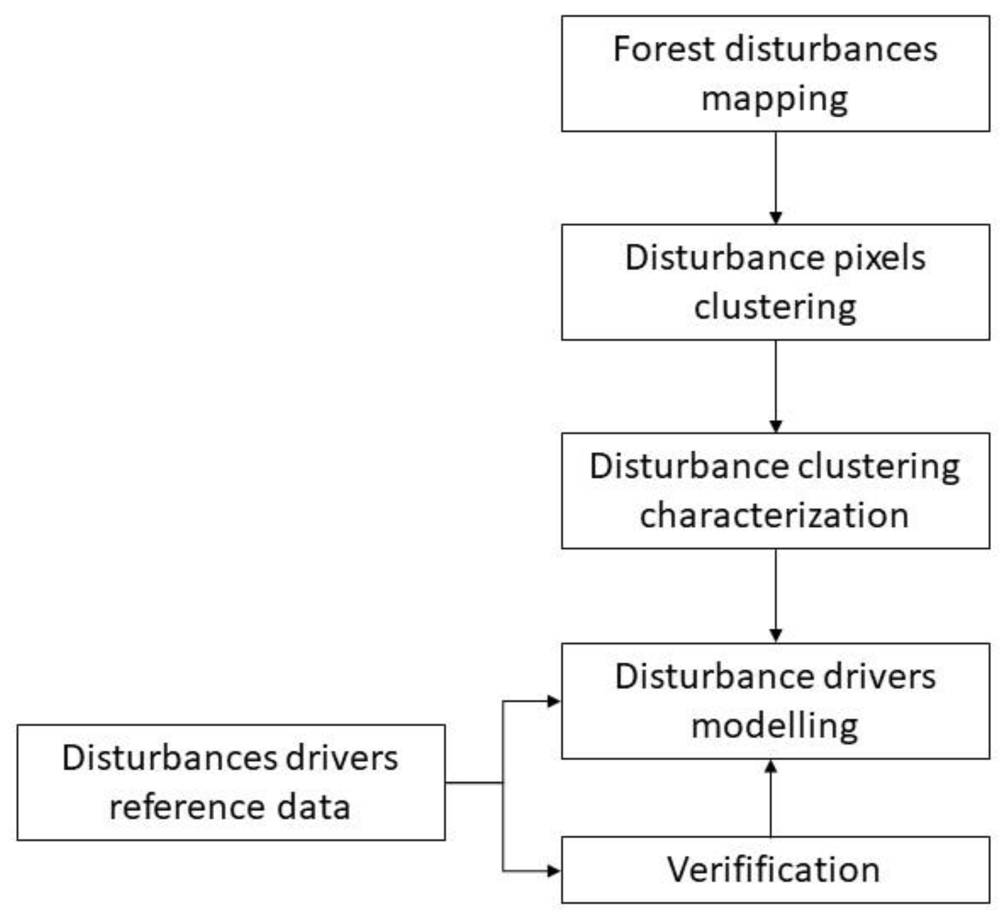
Sentinel-2 images were used in this study to perform the disturbance-detection-related steps. The data product used was the Level-2A, which includes geometric, radiometric and atmospheric corrections [48]. Images covering the whole study area were downloaded from the Copernicus Open Access Hub [49]. One image per month was downloaded for all the study years (2018, 2019 and 2020). The criteria to select the images were: for each month select the image with smallest percentage of cloud cover, discard images with a cloud cover smaller than 50% and finally if no image satisfies the maximum cloud-cover criterion, select an image at the end of the previous month or at the beginning of the following month.
Information from the European Forest Fire Information System (EFFIS) [50] was used as complementary data to obtain the location of wildfires that took place in Galicia during the period analyzed.
Information related to harvesting locations was obtained from one of the regional government’s databases, which is shared by the Xunta de Galicia in the context of the “Galician continuous forest inventory” project [51]. It consisted of a set of cadastral reference numbers where harvesting licenses were granted during the period from 2017 to 2019. This information was cross-referenced with the Spanish cadastral geodatabase [47] to obtain the exact location of the harvesting activities.
The information obtained from these two sources was contrasted using VHR aerial orthorectified images (PNOA images) dating from 2017 and from 2020 [52]. The images are available online through the Spanish National Cartographical Institute (IGN) [52]. The images from 2017 have a spatial resolution of 0.25 m and their georeferencing mean square error is ≤0.5 m. The images from 2020 have a spatial resolution of 0.15 m and a georeferencing mean square error of ≤0.20 m.

2.3. Main Method

This section describes the methodology to automatically obtain the driver of a forest disturbance, considering the forest disturbance map as the starting point. It might be highlighted that the methodology can be applied whatever procedure is followed to obtain the disturbances map. The first subsection (Section 2.3.1.) describes the particular procedural chain that was performed in this case to obtain the disturbance map of the study area, which is the region of Galicia. The following subsections (Section 2.3.2 and Section 2.3.3) are focused on describing in detail the proposed novel methodology to distinguish among forest disturbance drivers. A diagram of the main method is presented in Figure 2.

2.3.1. Forest Disturbance Mapping

The forest disturbance map of Galicia was obtained through the comparison of three consecutive annual land cover maps, specifically those corresponding to 2018, 2019 and 2020. The annual land cover maps were obtained according to the multitemporal approach described in Alonso et al. [53]. This approach was specifically designed to optimize the results considering the singularities of the Galician forest sector. It consists of performing supervised classifications of multi-temporal series of Sentinel-2 images. At first, one image is selected per single month for the study area; in that way, a group of twelve images is considered for every analyzed year. All the images are pre-processed to remove clouds using the cloud mask provided by the Sentinel Level 2A product. Secondly, a dataset of training pixels is defined for every year. In our case, it was performed through photointerpretation of the available PNOA images, dating from 2017 and from 2020 [52], as well as Sentinel-2 images. Contours of pixels with homogeneous land use were delineated to define the training polygons of the map classes. Once the 2019 training dataset was defined, it was used as a starting point for building the dataset for 2018 and 2020: considering the photointerpretation, the polygons were redefined if any land use change was appreciated. As a result, the size of training pixels datasets was similar for every classification. Thirdly, a supervised classification is performed on every single Sentinel image. For this end, bands with 10 m resolution were resampled to 20 m resolution using the nearest neighborhood interpolation. The classifications were performed applying the random forest algorithm [54]. As a result of this process, land cover maps are obtained for every single month. The last step is the aggregation of the 12 maps of a given year in a final map. This step was performed using the plurality voting decision criteria [53]. In that way, one aggregated map is obtained for every analyzed year. The three obtained maps were cross-verified using a set of points randomly distributed around the study area. The ground truth of those points for each year was obtained by photointerpretation of PNOA images from 2017 and from 2020 [52]. The cross-verification was performed trough the creation of a confusion matrix for each year.
Once land cover maps were obtained for 2018, 2019 and 2020, inter-annual comparisons were performed to detect potential land cover changes. For this end, pairs of maps were combined into a single raster file through a simple transformation and arithmetic raster calculation. A multiplication factor was applied to the raster file MAPyear1, and the result was added to the MAPyear2. A graphic illustration of this combination is presented in Figure 3. The digital values of the resulting raster file preserve the land cover classes of the two combined maps for every single pixel: the first digit of every pixel corresponds to the class of the earlier year, while the last digit corresponds to the class of the later year. In this way, changes involving vegetation reduction can be easily detected. For instance, pixels where a tree forest class has moved to any other non-tree class are considered disturbances, and pixels where shrubs have moved to another non-vegetated class are considered disturbances as well. Therefore, all the pixels that in 2018 had a forest-related cover (Eucalyptus spp., Conifer, Broadleaf or Shrub) and in 2019 had a land cover, which implied a vegetation reduction (shrubs, crop and pastures, bare soil or anthropogenic area), were considered as change pixels. The same criterion was followed to detect vegetation changes in the biennium in 2019–20. All the digital values reflecting these kind of changes were reclassified to obtain a binary result (0–1), and therefore obtain a disturbance/non-disturbance raster file. The analyzed bienniums were combined through raster layer addition. The result can be considered the disturbance map of the whole study area in the considered period.

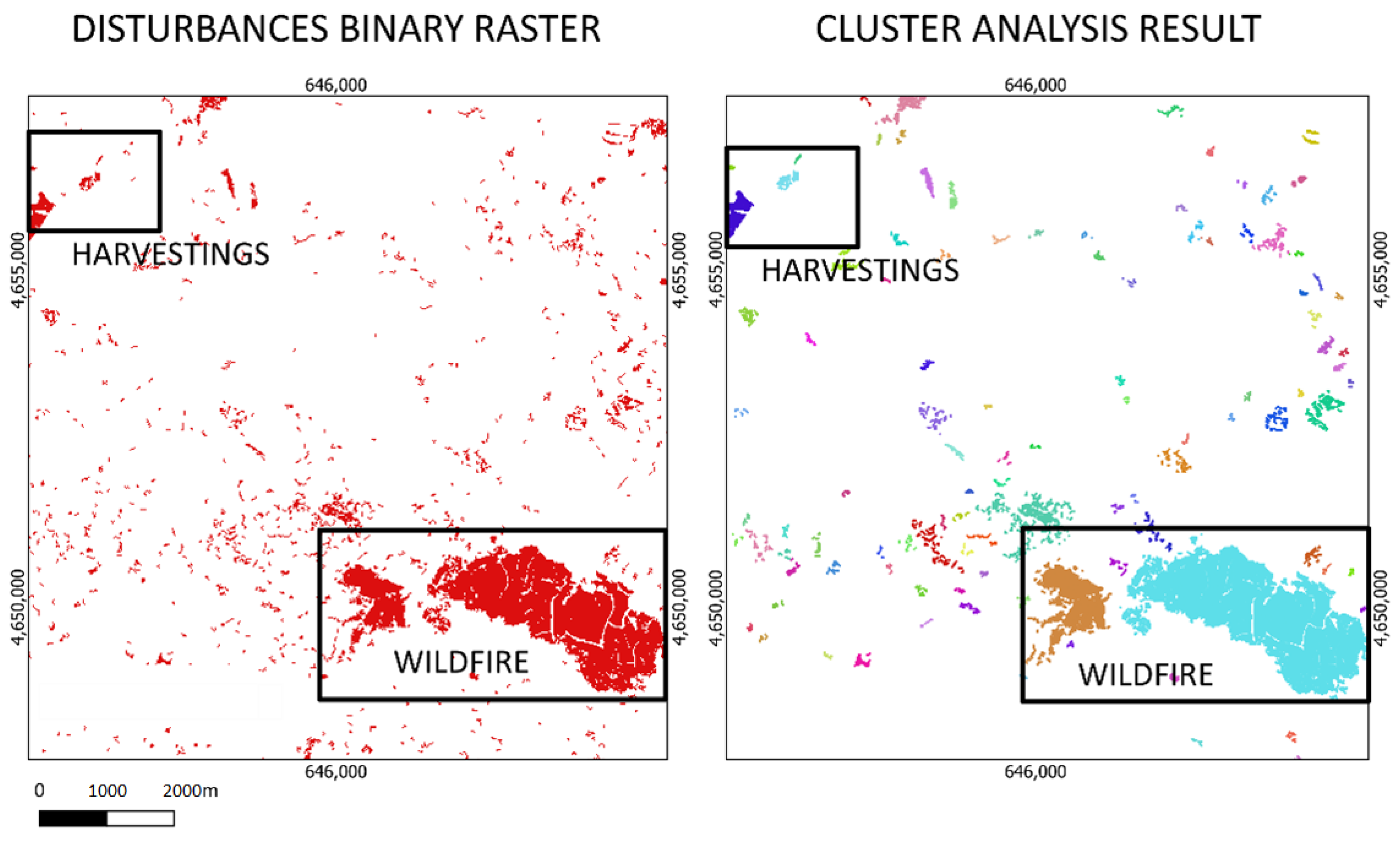
2.3.2. Disturbance Pixels Clustering

Once the forest disturbance map is available for the study area, the identification of the drivers can be accomplished over it. As previously pointed out, the subsequent procedure does not depend on the methodology that was followed to obtain the disturbances map. The only requirement is to arrange the disturbance raster layer in a binary format, where pixels with digital value 1 correspond to a disturbance occurring in the considered period and pixels with digital value 0 correspond to areas where forest vegetation has remained unaltered.
The first step to be accomplished is the clustering of those pixels of the disturbance map that correspond to the same disturbance event. This step is needed to be able to automatically individualize each disturbance event to further perform the geometrical characterization of each of them. The basic criterion to stablish the grouping is the proximity of pixels. A cluster analysis of the disturbance pixels was performed. The algorithm used was the Density-Based Cluster Algorithm (DBSCAN) [55]. This algorithm is an unsupervised learning method, which is efficient at finding clusters of arbitrary shape and when dealing with large databases. It allows to identify regions of high point density, which can be assimilated to disturbance events, and regions of low point density, where points do not have any other point close enough to be grouped in a cluster. Two parameters can be configured: the minimum number of points needed in a region to be considered dense (minPts) and a distance threshold above which it is not possible to consider two points to be neighbors (eps). Several values of both parameters might be tested to find a configuration that optimize the result for the study area. The result of this step is a map of forest disturbance events.

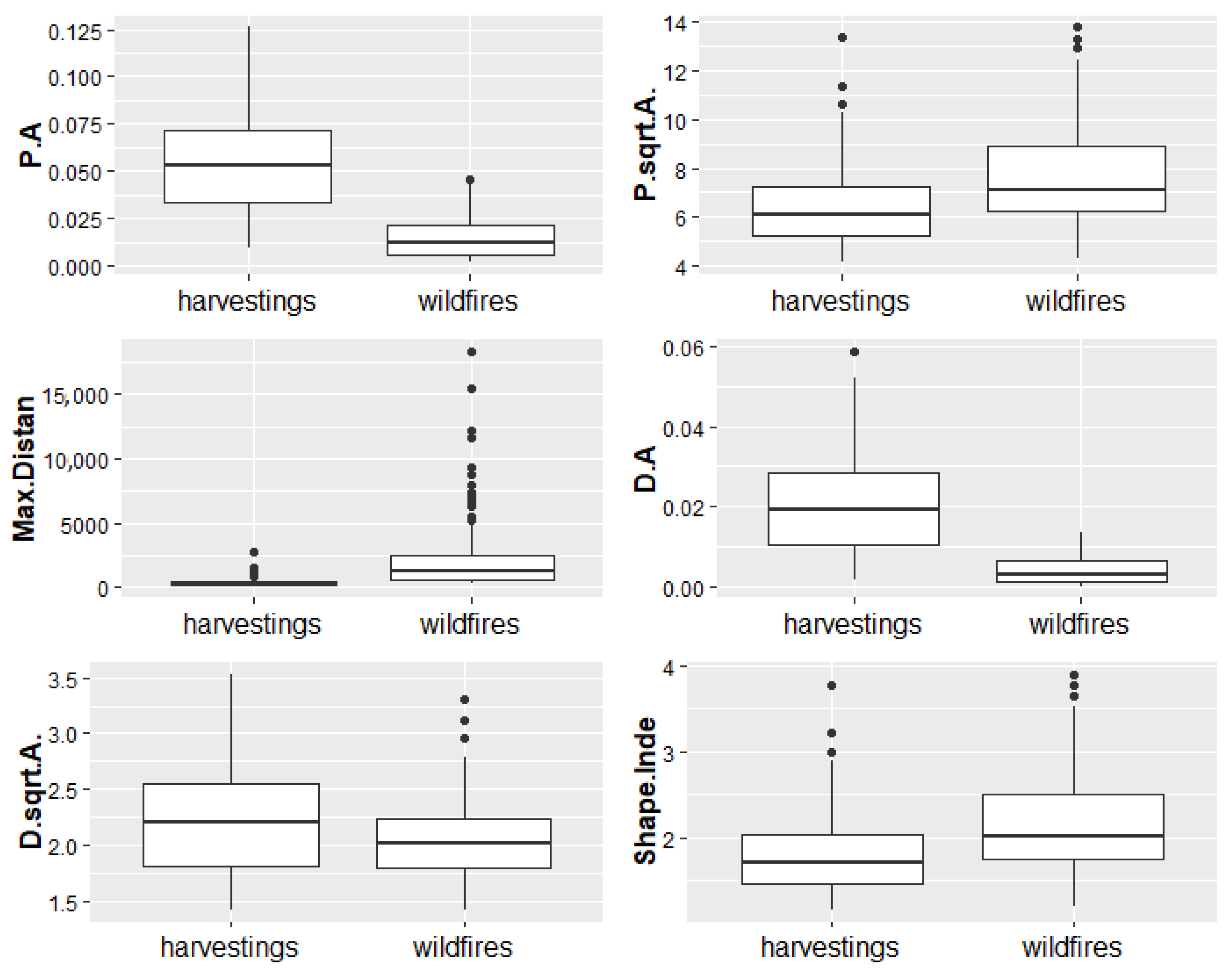
2.3.3. Disturbance Clusters Characterization

Once change disturbance events are mapped, they can be characterized in terms of shape-related and pattern-related metrics. According to previous experience, the shape of a wildfire usually tends to be close to an irregular ellipse with a large number of snags, resulting in a disturbance area with irregular boundaries [35,38,39]. On the contrary, harvesting tends to have a more regular shape and to form a continuous patch [35,38,39]. Several metrics were obtained to characterize every single disturbance cluster.
A first set of metrics was obtained to study how the pixels in each cluster in the map of forest disturbance events are distributed in relation to one another. All metrics were based on a previously calculated distance matrix containing the Euclidean distance between each pair of pixels in a cluster. The diagonal of the obtained distance matrix was set to NoData to avoid including distances of 0 in the subsequent calculations. The metrics obtained are presented in Table 1.
A second set of metrics for all the clusters present in the map of forest disturbance events was calculated. This one was focused on metrics related to the distance from each pixel in the cluster to the center of gravity of the cluster. Therefore, the center of gravity of each cluster was calculated and afterwards metrics presented in Table 2 were calculated:
An additional set of metrics was calculated for all the clusters present in the map of forest disturbance events, based on the polygon formed by each cluster. To obtain this polygon for each cluster, the concave hull [56] of the polygon of the cluster was calculated using the k-nearest neighbor approach to compute the region occupied by a set of points. The value of k is used to control the concaveness of the output polygon, resulting in the “smoothest” polygon when the lowest k value is used. In this study, k was set to 3. Using the resulting polygons, the shape metrics presented in Table 3 were calculated for each cluster.
2 ( A π ) / P
Equation (1). Equation of the Shape Index. A stands for the area of the polygon. P stands for the perimeter. Equation from [57].

2.3.4. Disturbance Drivers Modeling (Wildfires or Harvesting)

This step aims at classifying forest disturbance events into wildfires or harvestings considering the obtained shape and pattern metrics. For this end, a ground truth dataset is required. It was built by selecting clusters in the map of forest disturbance events and assigning them to either wildfires or harvestings. Wildfires were identified through the EFIS geodatabase [50]. Harvesting areas were identified through the information provided by the Xunta de Galicia [51]. The information provided by these two external sources was verified and filtered through photointerpretation by comparing the 2017 PNOA [52] and the 2020 PNOA [52]. Finally, a total of 304 clusters were selected, 170 corresponding to wildfires and 134 to harvesting areas. Although the sample might seem scarce, it was not augmented to avoid having a big class imbalance. A bigger amount of harvesting reference data was available but more records of wildfires during the study period were not found.
The modeling technique used was decision-tree learning through the building of a classification tree. This technique predicts the value of a target variable by learning simple decision rules inferred from the features of the data [58]. This technique was selected due to its simplicity of implementation and interpretation. In fact, there exists previous scientific literature related with land forest disturbances that relies on this technique [59,60]. In order to implement it, the ground truth set of data was randomly divided into training and verification datasets. Seventy percent of the clusters were used to train the decision tree and the other 30% were used to verify it. The decision tree was built on the training dataset using the default parameters of the “rpart” library of the R software [61]. This library also allows to calculate the variable importance of all the variables that formed the tree, understood as “the sum of the goodness of split measures for each split for which it was the primary variable, plus the adjusted agreement for all splits in which it was a surrogate”. The library scales the results to sum 100 and omits the variables with an importance smaller than 1%.
The resulting decision tree allowed to classify the disturbances and obtain a map of wildfires and harvestings. This map was cross-verified with the remaining ground truth subset. A confusion matrix was built, and the following accuracy metrics were obtained: Overall Accuracy (OA), Users Accuracy (UA), Producers Accuracy (PA) and Kappa Index. As the decision tree created may change as the training dataset changes, the presented modeling steps were repeated several times in order to obtain multiple decision trees and multiple sets of accuracy metrics. Finally, the decision tree that produced the best accuracy metrics was selected.

3. Results

This section is divided in four subsections. In Section 3.1. results of the disturbances mapping are presented. The next section, Section 3.2., focuses on presenting the results of the disturbance clustering procedure. Section 3.3. analyzes the behavior of the shape-related metrics calculated for the clusters presented in the previous section depending on their disturbance nature (harvestings or wildfire). The final section presents the results of the disturbance drivers modelling step.

3.1. Disturbances Mapping

The annual land cover maps were obtained for the whole study area following the methodology described in the previous section. The considered map classes were: conifers, Eucalyptus spp., other broadleaves, shrubs, crops and pastures, bare soils, anthropogenic areas and water bodies. A total of 1671 random points were obtained to perform the cross-verification. The estimated overall accuracy obtained for each map was: 78% for the 2018 map and 79% for both 2019 and 2020 maps.
The comparison of consecutive annual maps was performed to obtain the disturbances map. The result is a binary raster file showing all the pixels where the vegetation was significantly reduced. The raster layer addition of the disturbances map corresponding to 2018–19 and the disturbances map of 2019–20 results in the final disturbance map for the study area in the analyzed period. An example is shown in Figure 4.

3.2. Disturbances Clustering

As a result of the cluster analysis, a total of 25,307 disturbance clusters were obtained for the period of 2018–2020. An example of several of the clusters obtained is shown in Figure 5. The configuration parameters that optimize the results considering the singularities of the disturbances in the study area were: 10 minPts and 100 eps. High minPts values involve wildfire ledges that are not considered individual disturbances (i.e., the ledge of the cyan blue wildfire cluster in Figure 5). Furthermore, close individual harvests are efficiently clustered together (i.e., marked harvests in Figure 5). Low eps values prevent large wildfires from being identified as single disturbances (i.e., wildfires marked in Figure 4 that correspond to one single wildfire event). It was observed that those clusters identified as wildfires maintained the typical shape and point distribution of a wildfire.

3.3. Disturbances Clusters Characterization

All the obtained clusters were characterized in terms of shape and pattern according to the metrics described in the previous section. In order to accomplish the subsequent step, consisting of modelling disturbances in the study area, the metrics of a ground truth dataset were analyzed in detail. For this end, 304 clusters were selected, 170 corresponding to wildfires and 134 to harvesting areas. They were identified using the complementary databases mentioned in Section 2.3.4 and filtered by photointerpretation. The metrics of these datasets are presented in Figure 6, Figure 7 and Figure 8. The paired boxplots clearly show which metrics present different values depending on the driver of the disturbance. Several Figures reveal that wildfires have more outstanding outliers than harvestings and sometimes they take values in a wider range (mdmax, mdsd, MaxDistan, etc.). This might be due to some metrics being highly related to the size of the event (for instance mdmax or dmaxCOG) and some others to the shape (mdmean, mdsd, etc.). The wildfires in the study area present an important variability of sizes and shapes; most of them affect small areas but some of them are large wildfires.
Figure 6 shows the paired boxplots obtained for the metrics related to how the points in each cluster are distributed in relation to one another. The metrics that seem to mostly differ between harvesting and wildfires are: mdmax, mdmean and mdsd. The larger values of mdmean in wildfires might be due to their irregular shapes, which involve larger medium distances among points. The larger values of mdmax in wildfires might be due to the occurrence of events with larger sizes than the size of harvestings. The combination of larger sizes and irregular shapes result in higher values of mdsd in wildfires.
Figure 7 shows the paired boxplots obtained for the metrics related to the distance from each point in the cluster to the center of gravity of the cluster. The metrics which present the least overlap between boxplots are dmaxCOG, dmeanCOG and dsdCOG. Here again it might be highlighted that the fact that dmaxCOG and dmeanCOG are larger in wildfires has to do with the larger size of wildfires and their more irregular shape.
Figure 8 shows the paired boxplots obtained for the metrics calculated focused on the shape of the polygon formed by the cluster. The greatest differences between the harvesting and wildfire boxplots can be seen in P.A and D.A followed by Max.Distan. In fact, above all the metrics presented, P.A and D.A are the ones that present the greatest differences. In small events, the quotient between perimeter and total area, or between diameter and total area is higher. Harvestings usually present smaller areas than wildfires, and this is reflected in their respective P.A and D.A boxplots.

3.4. Disturbance Driver Modeling (Wildfire or Harvesting)

Shape and pattern-based metrics of wildfires significantly differ from the characteristic metrics of harvestings. The decision tree that optimized the classification of disturbances according to its driver is shown in Figure 9. The metrics present in this tree are D.A, mdmin and P.A. This indicates that generally, when the relation between the diagonal of the polygon formed by the cluster of a disturbance and the area of the polygon is greater than 0.01, that the disturbance is harvesting; however, when this relation is smaller, more conditions must be analyzed. First, if the average of the mdmin is relatively large (>30), it is a wildfire. If it is not, an additional condition needs to be analyzed. This last condition is the relation between the perimeter and the area of the polygon that is formed by the cluster (P.A). If this relation is smaller than 0.014, the disturbance is a wildfire; on the contrary, it is a harvesting event.
The variable importance results are presented in Figure 10. Variables with a greater importance are D.A. and P.A., followed by Max.Distan and mdmax. It might be highlighted that although mdmin forms parts of the final decision tree, its importance by itself is around 10%.
The confusion matrix obtained by applying this decision tree to the test points is presented in Table 4. In general, high accuracy metrics were obtained. The OA was 91% and the UA and the PA range between 87% and 94%. The Kappa Index obtained was 0.82.

4. Discussion

The shape and pattern metrics of disturbances revealed that wildfires in the study area tend to affect larger surfaces and/or affected areas and present larger extensions than harvestings, which tend to present more regular shapes than wildfires. This analysis is aligned with previous experiences [35,38,39].
High accuracy metrics were obtained (OA 91%) for distinguishing between wildfires and harvesting through the study of the geometry and shape of these disturbances. This high OA accuracy and the accompanying high UA and PA high-accuracy metrics (between 87% and 94%) indicate that the described methodology could help to distinguish between wildfires and harvestings once a disturbance map was obtained. Besides, this indicates that, as previously pointed out, wildfires and harvesting tend to have different shapes [35,38,39], a fact that aids in associating a driver to each disturbance. In fact, Hermosilla et al. [36] already identified that some geometric metrics (area and compactness) could aid in attributing a driver to a disturbance. In this study, different metrics (D.A, mdmin and P.A) have been found useful. The fact that other geometric metrics were useful in a quite different study area (the boreal forest in Canada) indicates that the application of this method in different biomes and study areas should be further studied in more detail, as wildfire regimes and harvesting practices can greatly differ among biomes resulting in disturbances that respond to different spatial patterns [6,62]. Such research would assess the adaptation of the method to different realities, contemplate the introduction of different metrics and identify which decision tree would best suit each different situation.
Although decision-tree algorithms were found useful in this study, there exists the possibility of testing different machine learning algorithms. For example, Random forest [54], a widely used machine learning algorithm in disturbance-related scientific works [63,64]. Besides, by using such algorithms, the repetition of the modelling steps to select the tree that retrieved better results could be avoided as this algorithm is based on the combination of multiple decision trees.
One of the key points in the described methodology is the aggregation of change pixels to individualize disturbance events. This step is needed in any disturbance driver attribution methodology that relies on the disturbance’s geometry and shape. A novel way of performing this step has been described here (cluster analysis). The main advantage of this method is that it can be used with any change-detection method relying on remote-sensing imagery, whereas, in previous studies, the individualization of a disturbance was dependent upon knowledge of the date and duration of the event [35,36]. This meant that, while many other methods have been successfully developed, the change detection in these studies had to be performed mainly by dense time-series analyses [16,65]. The fully automatic methodology described here could be used in conjunction with any other type of change-detection methodology so long as its result contains the localization of the change pixels. The main difficulty that the cluster analysis may represent is pinpointing the optimum configuration of the cluster algorithm parameters to correctly individualize disturbances. It was found that with the parameters selected in this study, some areas of the disturbance events were detached into different clusters (i.e., in the case of large wildfires) and that disturbances smaller than 4 ha were not detected due to the need for setting the minpts to 10. Nonetheless, for detecting wildfires, the selected parameters confer an improvement in terms of scale when compared with studies using other databases, for example those that rely on MODIS data (250 m spatial resolution) [50]. Therefore, further research should be conducted to fine-tune this step and improve the cluster results as well as to include small disturbances in the analysis and test the methodology in such cases.

5. Conclusions

A novel method based on the analysis of the shape and geometrical pattern of forest disturbances was described. It allows to identify whether forest disturbances have been driven by wildfire or by harvesting. High accuracy metrics were obtained for the study case, displaying the effectiveness of the methodology. The main novelty of this approach relies on the single use of geometrical and shape metrics of forest disturbances. The main advantages of the method are its ability to fully automate the process of distinguishing between drivers, and the possibility of applying it to any set of forest changes regardless of the remote-sensing-based method used to detect them. This may be a major advantage, as different study areas might require the use of different methodologies to detect forest disturbances due to different climatic conditions (e.g., the continuous presence of clouds) or landscape configurations (e.g., high fragmentation), among others. For our record, this is the first method to derive forest disturbance drivers that is not linked with the methodology followed to obtain the disturbances. Besides, the methodology is highly affordable, as it does not require additional sets of data, and it can be performed in near real-time as soon as the disturbances are detected. Advances such as this one in forest disturbance driver detection could be essential in aiding national and international agencies incorporate this information into their forest-related reports. Therefore, further studies on drivers and the utility of the geometric properties of disturbances in different biomes and study areas would be relevant. This will aid in the design of management actions aimed at improving forest sustainability as well as in the decision-making process of designing responses to the disturbances, thus contributing to the preservation of forests and supporting their key roles in the current context of climate change.

Author Contributions

Conceptualization, L.A. and J.A.; methodology, L.A. and J.A.; software, L.A.; validation, L.A.; formal analysis, L.A.; investigation, L.A.; resources, J.A. and J.P.; data curation, L.A.; writing—original draft preparation, L.A.; writing—review and editing, L.A. and J.A.; visualization, L.A.; supervision, J.A. and J.P.; project administration, J.A. and J.P.; funding acquisition, J.A. and J.P. All authors have read and agreed to the published version of the manuscript.

Funding

This research was funded by the Administration of Rural Areas of the Government of Galicia under Grant 2020CONVINVENTARIOFORESTALR002; the Spanish Ministry of Sciences, Innovation and Universities under Grant FPU19/02054; EP-INTERREG V A España Portugal (POCTEP) under grant FIREPOCTEP; Spanish Ministry of Sciences, Innovation and Universities under Grant PID2019-111581RB-I00.

Institutional Review Board Statement

Not applicable.

Informed Consent Statement

Not applicable.

Data Availability Statement

The data presented in this study are openly available in Copernicus Open Access Hub (https://scihub.copernicus.eu/dhus/#/home, accessed on 3 November 2021) [51].

Conflicts of Interest

The authors declare no conflict of interest.

References

  1. Pan, Y.; Birdsey, R.; Fang, J.; Houghton, R.; Kauppi, P.; Kurz, W.; Phillips, O.; Shvidenko, A.; Lewis, S.; Canadell, J.; et al. Large and Persistent Carbon Sink in the World’s Forests. Science 2011, 333, 988–993. [Google Scholar] [CrossRef] [Green Version]
  2. Forests in focus. Nat. Clim. Chang. 2021, 11, 363. [CrossRef]
  3. Ingalls, M.L.; Dwyer, M.B. Missing the forest for the trees? Navigating the trade-offs between mitigation and adaptation under REDD. Clim. Chang. 2016, 136, 353–366. [Google Scholar] [CrossRef]
  4. Seidl, R.; Thom, D.; Kautz, M.; Martin-Benito, D.; Peltoniemi, M.; Vacchiano, G.; Wild, J.; Ascoli, D.; Petr, M.; Honkaniemi, J.; et al. Forest disturbances under climate change. Nat. Clim. Chang. 2017, 7, 395–402. [Google Scholar] [CrossRef] [PubMed] [Green Version]
  5. FAO. Better Data, Better Decisions. Towards Impactful Forest Monitoring; Forestry Working Paper No. 16.; FAO: Rome, Italy, 2020. [CrossRef]
  6. Senf, C.; Seidl, R. Mapping the forest disturbance regimes of Europe. Nat. Sustain. 2021, 4, 63–70. [Google Scholar] [CrossRef]
  7. United Nations. Paris Agreement. 2015. Available online: https://unfccc.int/process-and-meetings/the-paris-agreement/the-paris-agreement (accessed on 29 October 2021).
  8. United Nations Department of Economic and Social Affairs. The Global Forest Goals Report 2021. Realizing the Importance of Forests in a Changing World; UN: New York, NY, USA, 2021; ISBN 9789214030515. [Google Scholar] [CrossRef]
  9. Seidl, R.; Honkaniemi, J.; Aakala, T.; Aleinikov, A.; Angelstam, P.; Bouchard, M.; Boulanger, Y.; Burton, P.J.; De Grandpré, L.; Gauthier, S.; et al. Globally consistent climate sensitivity of natural disturbances across boreal and temperate forest ecosystems. Ecography 2021, 43, 967–978. [Google Scholar] [CrossRef]
  10. Wang, J.A.; Baccini, A.; Farina, M.; Randerson, J.T.; Friedl, M.A. Disturbance suppresses the aboveground carbon sink in North American boreal forests. Nat. Clim. Chang. 2021, 11, 435–441. [Google Scholar] [CrossRef]
  11. Dupuy, J.-L.; Fargeon, H.; Martin-StPaul, N.; Pimont, F.; Ruffault, J.; Guijarro, M.; Hernando, C.; Madrigal, J.; Fernandes, P. Climate change impact on future wildfire danger and activity in southern Europe: A review. Ann. For. Sci. 2020, 77, 35. [Google Scholar] [CrossRef]
  12. Moraes, I.; Azevedo-Ramos, C.; Pacheco, J. Public forests under threat in the Brazilian Amazon: Strategies for coping shifts in environmental policies and regulations. Front. For. Glob. Chang. 2021, 4, 631756. [Google Scholar] [CrossRef]
  13. Mitchell, A.L.; Rosenqvist, A.; Mora, B. Current remote sensing approaches to monitoring forest degradation in support of countries measurement, reporting and verification (MRV) systems for REDD++. Carbon Balance Manag. 2017, 12, 9. [Google Scholar] [CrossRef] [Green Version]
  14. Regulation (EU) No 995/2010 of the European Parliament and of the Council of 20 October 2010 Laying down the Obligations of Operators Who Place Timber and Timber Products on the Market; Official Journal of the European Union; European Union: Maastricht, The Netherlands, 2010.
  15. Wulder, M.A.; Coops, N.C.; Roy, D.P.; White, J.C.; Hermosilla, T. Land cover 2.0. Int. J. Remote Sens. 2018, 39, 4254–4284. [Google Scholar] [CrossRef] [Green Version]
  16. Hirschmugl, M.; Gallaun, H.; Dees, M.; Datta, P.; Deutscher, J.; Koutsias, N.; Schardt, M. Methods for Mapping Forest Disturbance and Degradation from Optical Earth Observation Data: A Review. Curr. For. Rep. 2017, 3, 32–45. [Google Scholar] [CrossRef] [Green Version]
  17. Masiliūnas, D.; Tsendbazar, N.-E.; Herold, M.; Verbesselt, J. BFAST Lite: A Lightweight Break Detection Method for Time Series Analysis. Remote Sens. 2021, 13, 3308. [Google Scholar] [CrossRef]
  18. Verbesselt, J.; Hyndman, R.; Newnham, G.; Culvenor, D. Detecting trend and seasonal changes in satellite image time series. Remote Sens. Environ. 2010, 114, 106–115. [Google Scholar] [CrossRef]
  19. Verbesselt, J.; Zeileis, A.; Herold, M. Near real-time disturbance detection using satellite image time series. Remote Sens. Environ. 2012, 123, 98–108. [Google Scholar] [CrossRef]
  20. Kennedy, R.E.; Yang, Z.; Cohen, W.B. Detecting trends in forest disturbance and recovery using yearly Landsat time series: 1. LandTrendr—Temporal segmentation algorithms. Remote Sens. Environ. 2010, 114, 2897–2910. [Google Scholar] [CrossRef]
  21. Zhu, Z.; Woodcock, C.E. Continuous change detection and classification of land cover using all available Landsat data. Remote Sens. Environ. 2014, 144, 152–171. [Google Scholar] [CrossRef] [Green Version]
  22. Bustamante, M.M.C.; Roitman, I.; Aide, T.M.; Alencar, A.; Anderson, L.O.; Aragão, L.; Asner, G.P.; Barlow, J.; Berenguer, E.; Chambers, J.; et al. Toward an integrated monitoring framework to assess the effects of tropical forest degradation and recovery on carbon stocks and biodiversity. Glob. Chang. Biol. 2016, 22, 92–109. [Google Scholar] [CrossRef]
  23. Bowd, E.J.; McBurney, L.; Blair, D.P.; Lindenmayer, D.B. Temporal patterns of forest seedling emergence across different disturbance histories. Ecol. Evol. 2021, 11, 9254–9292. [Google Scholar] [CrossRef]
  24. Dragotescu, I.; Kneeshaw, D.D. A comparison of residual forest following fires and harvesting in boreal forests in Quebec, Canada. Silva Fenn. 2012, 46, 365–376. [Google Scholar] [CrossRef] [Green Version]
  25. Kissinger, G.; Herold, M.; De Sy, V. Drivers of Deforestation and Forest Degradation: A Synthesis Report for REDD+ Policymakers; Lexeme Consulting: Vancouver, BC, Canada, 2012. [Google Scholar]
  26. Patacca, M.; Schelhaas, M.; Zudin, S.; Lindner, M. Database on Forest Disturbances in Europe (DFDE)—Technical Report; Project I-Maestro (ERA-NET Cofund ForestValue); European Forest Institute: Joensuu, Finland, 2020; 18p. [Google Scholar]
  27. Forzieri, G.; Pecchi, M.; Girardello, M.; Mauri, A.; Klaus, M.; Nikolov, C.; Rüetschi, M.; Gardiner, B.; Tomaštík, J.; Small, D.; et al. A spatially explicit database of wind disturbances in European forests over the period 2000–2018. Earth Syst. Sci. Data 2020, 12, 257–276. [Google Scholar] [CrossRef] [Green Version]
  28. Ceccherini, G.; Duveiller, G.; Grassi, G.; Lemoine, G.; Avitabile, V.; Pilli, R.; Cescatti, A. Abrupt increase in harvested forest area over Europe after 2015. Nature 2020, 583, 72–77. [Google Scholar] [CrossRef]
  29. Schepaschenko, D.; See, L.; Lesiv, M.; Bastin, J.-F.; Mollicone, D.; Tsendbazar, N.-E.; Bastin, L.; McCallum, I.; Bayas, J.C.L.; Baklanov, A.; et al. Recent Advances in Forest Observation with Visual Interpretation of Very High-Resolution Imagery. Surv. Geophys. 2019, 40, 839–862. [Google Scholar] [CrossRef] [Green Version]
  30. Key, C.H.; Benson, N.C. Measuring and remote sensing of burn severity. In Joint Fire Science Conference and Workshop; Neuenschwander, L.F., Ryan, K.C., Eds.; University of Idaho: Moscow, ID, USA, 1999; Volume 2. [Google Scholar]
  31. Haywood, A.; Verbesselet, J.; Baker, P.J. Mapping disturbance dynamics in wet sclerophyll forests using time series Landsat. Int. Arch. Photogramm. Remote Sens. Spatial Inf. Sci. 2016, XLI-B8, 633–641. [Google Scholar] [CrossRef] [Green Version]
  32. Esteban, J.; Fernández-Landa, A.; Tomé, J.L.; Gómez, C.; Marchamalo, M. Identification of Silvicultural Practives in Mediterranean Forests Integrating Landsat Time Series and a Single Coverage of ALS Data. Remote Sens. 2021, 13, 3611. [Google Scholar] [CrossRef]
  33. Moisen, G.G.; Meyer, M.C.; Schroeder, T.A.; Liao, X.; Schleeweis, K.G.; Freeman, E.A.; Toney, C. Shape selection in Landsat time series: A tool for monitoring forest dynamics. Glob. Chang. Biol 2016, 22, 3518–3528. [Google Scholar] [CrossRef] [PubMed]
  34. Schroeder, T.A.; Schleeweis, K.G.; Moisen, G.G.; Toney, C.; Cohen, W.B.; Freeman, E.A.; Yang, Z.; Huang, C. Testing a Landsat-based approach for mapping disturbance causality in U.S. forests. Remote Sens. Environ. 2017, 195, 230–243. [Google Scholar] [CrossRef] [Green Version]
  35. Schroeder, T.A.; Wulder, M.A.; Healey, S.P.; Moisen, G.G. Mapping wildfire and clearcut harvest disturbances in boreal forests with Landsat time series data. Remote Sens. Environ. 2011, 115, 1421–1433. [Google Scholar] [CrossRef]
  36. Hermosilla, T.; Wulder, M.A.; White, J.C.; Coops, N.C.; Hobart, G.W. Regional detection, characterization, and attribution of annual forest change from 1984 to 2012 using Landsat-derived time-series metrics. Remote Sens. Environ. 2015, 170, 121–132. [Google Scholar] [CrossRef]
  37. Neigh, C.S.R.; Bolton, D.K.; Williams, J.J.; Diabate, M. Evaluating an Automated Approach for Monitoring Forest Disturbances in the Pacific Northwest from Logging, Fire and Insect Outbreaks with Landsat Time Series Data. Forests 2014, 5, 3169–3198. [Google Scholar] [CrossRef] [Green Version]
  38. Mcrae, D.J.; Duchesne, L.C.; Freedman, B.; Lynham, T.J.; Woodley, S. Comparisons between wildfire and forest harvesting and their implications in forest management. Environ. Rev. 2011, 9, 223–260. [Google Scholar] [CrossRef]
  39. Delong, S.C.; Tanner, D. Managing the pattern of forest harvest: Lessons from wildfire. Biodivers. Conserv. 1996, 5, 1191–1205. [Google Scholar] [CrossRef]
  40. Consellería do Medio Rural, Xunta de Galicia. 1a Revisión Del Plan Forestal de Galicia. 2015. Available online: https://mediorural.xunta.gal/fileadmin/arquivos/forestal/ordenacion/1_REVISION_PLAN_FORESTAL_CAST.pdf (accessed on 3 November 2021).
  41. Xunta de Galicia. Sistema de Indicadores da Administración Dixital. Producción Forestal. Available online: https://indicadores-forestal.xunta.gal/portal-bi-internet/dashboard/Dashboard.action?selectedScope=OBSFOR_BI_A02_INT&selectedLevel=OBSFOR_BI_2_INT.L0&selectedUnit=12&selectedTemporalScope=2&selectedTemporal=31/12/2020 (accessed on 3 December 2021).
  42. MAPA (Ministerio de Agricultura Pesca y Alimentación). Mapa Forestal de España a Escla 1:25.000 (MFE25). Available online: https://www.mapa.gob.es/es/desarrollo-rural/temas/politica-forestal/inventario-cartografia/mapa-forestal-espana/mfe_25.aspx (accessed on 3 November 2021).
  43. MAPA. Los Incendios Forestales en España. Decenio 2006–2015; MAPA: Madrid, Spain, 2019.
  44. MAPA. Estadísticas de Incendios Forestales. Available online: https://www.miteco.gob.es/es/biodiversidad/estadisticas/Incendios_default.aspx (accessed on 3 November 2021).
  45. MITERD. Anuario de Estadística Forestal 2018. Available online: https://www.mapa.gob.es/es/desarrollorural/estadisticas/aef_2018_documentocompleto_tcm30-543070.pdf (accessed on 21 July 2021).
  46. Levers, C.; Verkerk, H.; Müller DVerburg, P.; Butsic VLeitão, P.; Lindner, M.; Kuemmerle, T. Drivers of forest harvesting intensity patterns in Europe. For. Ecol. Manag. 2014, 315, 160–172. [Google Scholar] [CrossRef]
  47. Gobierno de España. Ministerio de Hacienda. Sede Electrónica del Catastro. 2011. Available online: https://www.sedecatastro.gob.es (accessed on 3 November 2021).
  48. ESA. European Comission. Sentinel-2. Available online: https://sentinels.copernicus.eu/web/sentinel/missions/sentinel-2 (accessed on 3 November 2021).
  49. ESA (European Space Agency). Copernicus and European Comission. Copernicus Open Access Hub. Available online: https://scihub.copernicus.eu/dhus/#/home (accessed on 23 July 2021).
  50. Copernicus. European Forest Fire Information System EFFIS. Available online: https://effis.jrc.ec.europa.eu/ (accessed on 3 November 2021).
  51. Xunta de Galicia. Consellería do Medio Rural, Inventario Forestal Continuo de Galicia (IFG). Available online: https://mediorural.xunta.gal/gl/temas/forestal/inventario-forestal-continuo (accessed on 3 November 2021).
  52. MTMAU (Ministerio de Transporte Movilidad y Agenda Urbana). Plan Nacional de Ortofotografía Aérea (PNOA). Available online: https://pnoa.ign.es/ (accessed on 23 July 2021).
  53. Alonso, L.; Picos, J.; Armesto, J. Forest Land Cover Mapping at a Regional Scale Using Multi-Temporal Sentinel-2 Imagery and RF Models. Remote Sens. 2021, 13, 2237. [Google Scholar] [CrossRef]
  54. Breiman, L. Random Forests. Machine Learning 2001, 45, 5–32. [Google Scholar] [CrossRef] [Green Version]
  55. Ester, M.; Kriegel, H.P.; Sander, J.; Xu, X. A density-based algorithm for discovering clusters in large spatial databases with noise. In Proceedings of the Second International Conference on Knowledge Discovery and Data Mining (KDD’96); AAAI Press: Portland, Oregon, 1996; pp. 226–231. [Google Scholar]
  56. Moreira, A.J.C.; Santos, M.Y. Concave hull: A k-nearest neighbours approach for the computation of the region occupied by a set of points. In GRAPP 2007, Proceedings of the Second International Conference on Computer Graphics Theory and Applications; Barcelona, Spain, 8–11 March 2007.
  57. Forman, R.T.T.; Godron, M. Landscape Ecology; John Wiley & Sons: New York, NY, USA, 1986. [Google Scholar]
  58. Breiman, L.; Friedman, J.H.; Olshen, R.A.; Stone, C.J. Classification and Regression Trees; Wadsworth: Boca Raton, FL, USA, 1984. [Google Scholar]
  59. Jin, S.; Yang, L.; Zhu, Z.; Homer, C. A land cover change detection and classification protocol for updating Alaska NLCD 2001 to 2011. Remote Sens. Environ. 2017, 195, 44–55. [Google Scholar] [CrossRef]
  60. López-Amoedo, A.; Álvarez, X.; Lorenzo, H.; Rodríguez, J.L. Multi-Temporal Sentinel-2 Data Analysis for Smallholding Forest Cut Control. Remote Sens. 2021, 13, 2983. [Google Scholar] [CrossRef]
  61. Therneau, T.; Atkinson, B. Rpart: Recursive Partitioning and Regression Trees. R Package Version 4.1-15. 2019. Available online: https://CRAN.R-project.org/package=rpart (accessed on 27 January 2021).
  62. Senf, C.; Seidl, R. Natural disturbances are spatially diverse but temporally synchronized across temperate forest landscapes in Europe. Glob. Chang. Biol. 2018, 24, 1201–1211. [Google Scholar] [CrossRef]
  63. Murillo-Sandoval, P.J.; Hilker, T.; Krawchuk, M.A.; Van Den Hoek, J. Detecting and Attributing Drivers of Forest Disturbance in the Colombian Andes Using Landsat Time-Series. Forests 2018, 9, 269. [Google Scholar] [CrossRef] [Green Version]
  64. De Marzo, T.; Pflugmacher, D.; Baumann, M.; Lambin, E.F.; Gasparri, I.; Kuemmerle, T. Characterizing forest disturbances across the Argentine Dry Chaco based on Landsat time series. Int. J. Appl. Earth Obs. Geoinf. 2021, 98, 102310. [Google Scholar] [CrossRef]
  65. Zhu, Z. Change detection using landsat time series: A review of frequencies, preprocessing, algorithms, and applications. ISPRS J. Photogramm. Remote Sens. 2017, 130, 370–384. [Google Scholar] [CrossRef]
Figure 1. Study area. Galicia (Northwest of Spain).
Remotesensing 14 00697 g001
Figure 2. Diagram of the main method.
Remotesensing 14 00697 g002
Figure 3. Diagram of the procedure followed to perform the inter-annual comparisons between paired years in order to obtain the land cover changes. MAPyear1: land cover map of the earlier year of the bi-annual analyzed land. MAPyear2: land cover map of the later year of the bi-annual analyzed land.
Remotesensing 14 00697 g003
Figure 4. Land cover map of 2018, 2019, 2020 and disturbances map.
Remotesensing 14 00697 g004
Figure 5. Examples of the cluster analysis results. On the left: disturbances binary raster in red disturbance pixels. On the right: the result of the cluster analysis; all the pixels that belong to a cluster are shown in the same color. Examples of wildfires and harvesting disturbances and clusters are highlighted.
Remotesensing 14 00697 g005
Figure 6. Paired boxplots of the metrics calculated related to how the points in each cluster are distributed in relation to one another. Boxplots are median based.
Remotesensing 14 00697 g006
Figure 7. Paired boxplots of the metrics calculated related to the distance from each point in the cluster to the center of gravity of the cluster. Boxplots are median based.
Remotesensing 14 00697 g007
Figure 8. Paired boxplots of the metrics calculated focused on the shape of the polygon formed by the cluster. Boxplots are median based.
Remotesensing 14 00697 g008
Figure 9. Decision tree that allows for the differentiation between harvesting and wildfires using the shape-related metrics calculated. D.A: the maximum diameter of the polygon formed by the cluster, calculated as the maximum distance between the vertices of two parts of the polygon, divided by the area of the polygon. mdmin: the average of the minimum distance from each disturbance pixel to its nearest disturbance pixel in the disturbance. P.A: the perimeter of the polygon formed by the disturbance divided by the area of the polygon.
Remotesensing 14 00697 g009
Figure 10. Variables’ importance according to the decision-tree algorithm implemented through the library rpart [61]. Variables with importances’ smaller than 1% were omitted.
Remotesensing 14 00697 g010
Table 1. Set of metrics calculated for each detected disturbance cluster to study how the pixels of the cluster are distributed in relation to one another.
MetricDescription
mdminThe average of the minimum distance from each pixel to the nearest pixel in the cluster. To obtain this, a matrix was computed containing the distances from each pixel to its nearest pixel. Then the mean of the values contained in the minimum-distance matrix was calculated.
mdmaxThe average of the maximum distance from each pixel to the farthest pixel in the cluster. To obtain this, a matrix was computed containing the distance from each pixel to its farthest pixel. Then the mean of the values contained in the maximum-distance matrix was calculated.
mdmeanThe average of the average distances from each pixel to the rest of the cluster pixels. To obtain this, a matrix was computed containing the average of the distances from each pixel to the rest of the pixels. Then the mean of the values contained in the mean-distance matrix was calculated.
mdsdThe average of the standard deviation of the distances from each pixel to the rest of the cluster pixels. To obtain this, a matrix was computed containing the standard deviation of the distances from each pixel to the rest of the pixels. Then the mean of the values contained in the standard-deviation matrix was calculated.
mdkurThe average of the kurtosis of the distances from each pixel to the rest of the cluster pixels. To obtain this, a matrix was computed containing the kurtosis of the distances from each pixel to the rest of the pixels. Then the mean of the values contained in the kurtosis matrix was calculated.
mdskewThe average of the skewness of the distances from each pixel to the rest of the cluster pixels. To obtain this, a matrix was computed containing the skewness of the distances from each pixel to the rest of the pixels. Then the mean of the values contained in the skewness matrix was calculated.
Table 2. Set of metrics calculated for each detected disturbance cluster to study the position of pixels in the cluster in relation to the center of gravity of the cluster.
MetricDescription
dmeanCOGThe average distance from each of the cluster of pixels to the cluster’s center of gravity.
dminCOGThe distance from the closest cluster of pixels to the cluster’s center of gravity.
dmaxCOGThe distance from the farthest cluster of pixels to the cluster’s center of gravity.
dsdCOGThe standard deviation of the distances of each of the clusters of pixels to the cluster’s center of gravity.
dkurtCOGThe kurtosis of the distances of each of the clusters of pixels to the cluster’s center of gravity.
dskewCOGThe skewness of the distances of each of the clusters of pixels to the cluster’s center of gravity.
Table 3. Set of metrics calculated on the polygon formed by each disturbance cluster. The polygon was obtained from the concave hull of the disturbance pixel centers.
MetricDescription
P.AThe perimeter of the polygon divided by its area.
P.sqrt.AThe perimeter of the polygon divided by the square root of its area.
Max.DistanThe maximum diameter calculated as the maximum distance between the vertices of two of the polygon’s parts.
D.AThe Max.Distan divided by the area of the polygon.
D.sqrt.AThe Max.Distan divided by the square root of the polygon’s area.
Shape Index (Shap.Inde)The inverse of the ratio of the perimeter of the equivalent circle to the real perimeter. See Equation (1) [57].
Table 4. Confusion matrix resulting from the application of the decision tree that classifies disturbances according to their drivers (wildfires or harvesting) to the test set of data. PA: Producer’s Accuracy; UA: User’s Accuracy; OA: Overall Accuracy; KI: Kappa Index.
Ground Truth
Decision treeHarvestingsWildfiresTotalUA (%)
Harvestings3453987
Wildfires3495294
22Total375491
PA (%)9291 OA (%)91
KI0.82
Publisher’s Note: MDPI stays neutral with regard to jurisdictional claims in published maps and institutional affiliations.

