Impact of Vertical Profiles of Aerosols on the Photolysis Rates in the Lower Troposphere from the Synergy of Photometer and Ceilometer Measurements in Raciborz, Poland, for the Period 2015–2020

Abstract

The effect of the aerosol vertical distribution on photolysis frequencies of O₃ and NO₂ is studied. Aerosol measurements in Raciborz (50.08° N, 18.19° E), Poland, made using the CIMEL Sun photometer and collocated CHM-15k “Nimbus” ceilometer are analyzed for the period 2015–2020. Vertical profiles of the aerosol extinction are derived from the Generalized Retrieval of Atmosphere and Surface Properties (GRASP) algorithm combining the ceilometer measurements of the aerosol backscattering coefficient with the collocated CIMEL measurements of the columnar characteristics of aerosols. The photolysis frequencies are calculated at the three levels in the lower troposphere (the surface and 0.5 and 2 km above the surface) using a radiative transfer model, Tropospheric Ultraviolet and Visible (TUV), for various settings of aerosol optical properties in the model input. The importance of the aerosol vertical distribution on photolysis frequencies is inferred by analyzing statistics of the differences between the output of the model, including the extinction profile from the GRASP algorithm, and the default TUV model (based on columnar aerosol characteristics by the CIMEL Sun photometer and Elterman’s extinction profile). For model levels above the surface, standard deviation, 2.5th percentile, 97.5th percentile, and the extremes, calculated from relative differences between these input settings, are comparable with the pertaining statistical values for the input pair providing changes of photolysis frequencies only due to the variability of the columnar aerosol characteristics. This indicates that the vertical properties of aerosols affect the distribution of the photolysis frequencies in the lower troposphere on a similar scale to that due to variations in columnar aerosol characteristics.

1. Introduction

Solar radiation drives atmospheric chemistry through the photolysis of many key species. Concerning the ozone production in the lower atmosphere, the basic reactions are photolysis of ozone that produces O¹D, which further reacts with H₂O giving the hydroxyl (OH) radical (Reactions 1–2) and photolysis of NO₂ yielding O³P that reacts with O₂ to produce O₃ (Reactions 3–4). The hydroxyl radical is the important oxidant in the atmosphere affecting the concentrations of toxic gases (e.g., carbon monoxide) and greenhouse gases (e.g., methane) [1]. Reactions 3–4 are the basic source of ozone in the troposphere [2]. O₃ and NO₂ are key components measured at ground-based air quality monitoring stations to inform the public of atmospheric pollutions (exceedances above the norms), which could have serious health consequences [3].

O₃ + hν(λ < 320 nm) → O¹ + O₂

(1)

O¹D + H₂O → 2OH

(2)

NO₂ + hν(λ < 430 nm) → NO + O³P

(3)

O³P + O₂ → O₃

(4)

The photolysis intensity is calculated using the photolysis frequency, j, defined by the following formula [2]:

$$j=\underset{{\lambda }_1}{\overset{{\lambda }_2}{{\displaystyle \int }}}F\left(\lambda \right)\sigma \left(\lambda ,T\right)\phi \left(\lambda ,T\right)\mathrm{d}\lambda$$

(5)

F(λ) is the actinic flux dependent on wavelength, σ(λ, T) is the absorption cross-section of the considered species, and φ(λ, T) is the quantum yield of the photodissociation reaction product. λ and T denote wavelength and temperature, respectively. Values for σ (λ, T) and φ(λ, T) are based on results of laboratory experiments. The photolysis frequency for reaction R1, denoted j (O¹D), is driven by short wavelengths mainly in the UV-B range (290–315 nm) of solar radiation, where ozone absorption and Rayleigh and Mie scattering are large, whereas for reaction R3, j (NO₂) depends mostly on longer wavelengths (λ < 430 nm), i.e., not sensitive to ozone and less affected by the light scattering.

The photolysis frequencies of species important for tropospheric chemical modeling are rarely available from observations. It is possible to calculate the value of j at the ground level from the measured spectral actinic flux (SAF). Unique spectrophotometers were designed to be used in a variety of field experiments [4,5,6,7]. Placing the spectrophotometer on board a plane during flights in the troposphere is also an option to obtain vertical changes of SAF [8,9]. For higher levels, numerical models of radiation transfer through the atmosphere were frequently applied to estimate SAF vertical profiles. The Library for Radiative Transfer (LibRadtran) [10] and the Tropospheric Ultraviolet and Visible (TUV) [11] model were frequently used in such calculations with a default setting of the aerosol extinction profile (commonly marked as α-profile) based on a parameterization proposed by [12,13], respectively. For example, the LibRadtran and the TUV model were used in papers [8,14,15] and [7,16,17], respectively. The authors of [18] showed comparisons between photolysis frequencies with different parameterizations of the aerosol characteristics (including α-profile). The α-profile could be also inferred from measurements of the backscattered light emitted by ground-based LIDARs [15,19].

Tropospheric aerosols significantly influence photolysis rates especially in urban areas with severe aerosol pollution [7,20]. Observational data over Beijing showed that aerosols reduced j (O¹D) and j (NO₂) by ~30% under clear-sky conditions relative to an aerosol-free atmosphere [7]. Over European regions, a reduction of ~10% was reported, which is much smaller than that in China because of the lower aerosol loads [6,21]. However, for extreme cases (i.e., during high aerosol loads) a reduction up to ~40–50% was found in Europe [6,22].

The important parameters affecting photolysis frequencies are solar zenith angle (SZA), clouds, aerosol optical characteristics (AOCs), surface albedo, column content of ozone, and altitude [23,24]. The key AOCs to be considered for calculation of j values for this study are aerosol optical depth (AOD), single scattering albedo (SSA), and asymmetry factor (AF). AOD is the column integral of the α-profile depending on wavelength. If information on AOD is not available for the observation site, it could lead to an error of the actinic flux of up to 30% [25]. The AOD is usually higher for shorter wavelengths, and the wavelength dependence of AOD is described by the Ångström exponent (ÅE), as follows [26],

$$\frac{{\mathrm{AOD}}_{\lambda 1}}{{\mathrm{AOD}}_{\lambda 2}}={\left(\frac{{\lambda }_1}{{\lambda }_2}\right)}^{-\AA \mathrm{E}}$$

(6)

where AOD_λ1 and AOD_λ2 are the AODs for the wavelengths λ₁ and λ₂, respectively.

SSA is the ratio between the scattering extinction coefficient and the total extinction coefficient. For smaller SSA, the light absorption is higher, causing a reduction of the actinic flux [27]. The third key parameter of AOC is the aerosol asymmetry factor (AF) that describes the angular distribution of the scattered light and indicates whether the scattering is forward (toward the ground) or backward. Typically, columnar characteristics of aerosols are available for simulation studies as they are measured by the global AERONET network using CIMEL Sun photometers [28].

We present a model study of the aerosol effects on two key photolysis frequencies, j (O¹D) and j (NO₂), using the α-profile derived from the Generalized Retrieval of Atmosphere and Surface Properties (GRASP) algorithm, combining the ceilometer measurements of the aerosol backscattering coefficient with the collocated CIMEL measurements of columnar characteristics of aerosols. For cloud-free cases over Raciborz (Poland) in 2015–2020, simultaneous observations by the CIMEL Sun photometer and the CHM-15k “Nimbus” ceilometer provided input to the TUV model. Moreover, vertical changes of SSA and ÅE determined by the Modern-Era Retrospective Analysis for Research and Applications version 2 (MERRA-2) reanalysis were also inserted into the TUV model. The j values for the three levels in the lower troposphere (the surface, 0.5 km and 2 km above surface) were analyzed based on the TUV model simulations with different AOC input settings to find out the importance of the vertical distribution of AOC on the photolysis rate.

2. Instrumentation and Methodology

The Raciborz Observatory (50.08° N, 18.19° E) is a part of the Institute of Geophysics, Polish Academy of Sciences, observation network. Raciborz is a town in southern Poland, located at a depression between the Sudetes and the Carpathian Mountains, in close vicinity to highly urbanized and industrialized region of Silesia in Poland and Ostrava industrial zone in the Czech Republic. This region suffers from high aerosol concentrations [29]. However long-range aerosol transport is also observed at this site [30,31]. The observatory in Raciborz is equipped with a CHM-15k “Nimbus” ceilometer and a collocated triple Sun–Sky–Lunar CIMEL photometer.

2.1. Passive Remote Sensing

The Raciborz Observatory is a part of the AERONET network and continuously provides data (for over six years). Description of the network, its calibration and provided data products can be found in many papers, e.g., [28,32]. The instrument measures direct Sun radiation at several wavelengths for the estimation of spectral AOD. In addition to AOD, sky radiances are obtained in the almucantar configuration (i.e., for fixed elevation angle equal to actual solar elevation angle, and ±180° azimuthal sweeps) at 440, 675, 870, and 1020 nm. The spectral AODs, together with sky radiances, are then input to the AERONET retrieval algorithm, providing columnar values of aerosol size distribution and complex index of refraction, which are used for estimates of various AOCs, including those constituting TUV input, i.e., SSA, ÅE, AF, and albedo. The newest AERONET version 3 aerosol retrieval algorithm [33] was implemented to collect AOCs at 440 nm measured in Raciborz in the period 2015–2020. These data were taken from the AERONET web page [34]. AOD at 340 nm and ÅE for the 340–440 nm range were on the web page [35]. Level 1.5 data were used in this study as more aerosol data were available in this case compared to that for level 2.0. Level 1.5 data also contain valuable cloud-screened data useful for radiative transfer modeling, as mentioned in previous articles [15,36].

2.2. Active Remote Sensing

Aerosol vertical profiling in Raciborz is performed with Lufft’s CHM-15k “Nimbus” ceilometer. Ceilometers are designed primarily for measurements of cloud base height. However, in some cases, they can be used to obtain some information on the aerosols’ vertical structure, e.g., [19,37] and serves as a cost-effective, simple LIDAR instrument. Technical details of the CHM-15k “Nimbus” ceilometer and benefits of using LIDAR soundings of the atmospheric aerosols are shown in recent publications, e.g., [38,39]. In this work, we used ceilometer signals averaged over a 20 min time window centered around coincident CIMEL measurements. Figure 1 shows examples of the ceilometer profiles of the aerosol backscattering signal to be used in the aerosol extinction retrieval (Section 2.3). A multilayered structure of aerosols could be observed both on 29 August 2018 and 25 January 2020. A stronger signal originating from aerosol layering was observed in the former case.

2.3. GRASP

GRASP is an advanced software package (code) that utilizes a numerical inversion algorithm to retrieve aerosol properties, including size distribution, spectral refractive index, and surface parameters. It might be used for both satellite- and ground-based spectral and multi-angular remote sensing. The GRASP code consists of two independent modules, forward and inversion ones [40,41]. The forward module utilizes radiative transfer calculations for the simulation of radiative measurement for a given aerosol scenario/model, whilst the inversion module is used to minimize the differences between the observed and the simulated radiative signals obtained via the forward module.

GRASP, besides being used for satellite retrievals [40,42,43], may also utilize the synergy of Sun photometer measurements and LIDAR-based aerosol vertical profiling for the retrieval of aerosol microphysical and optical property profiles. A detailed description of the Generalized Aerosol Retrieval from Radiometer and Lidar Combined data (GARRLiC) algorithm, a part of the GRASP code, is given by [44,45]. GRASP allows for the independent retrieval of different aerosol populations, each with different microphysical properties such as shape, range of aerosol size distribution, and refractive index. Single-wavelength LIDAR/ceilometer measurements allow the retrieval of the vertical distribution of a single population of the aerosol [46,47]. This configuration is used in this study. The use of a simple, single-population aerosol model implies the linear relation between the aerosol’s mass concentration, volume concentration and extinction at each considered wavelength. It is possible to retrieve the α-profile but not the vertically resolved SSA and AF.

Figure 2 shows examples of the GRASP α-profiles and the Elterman’s α-profile, the default α-profile in the TUV model (see Section 2.5). It is worth mentioning that the integral of the α-profile with the height (i.e., AOD value) is the same in both cases. The GRASP α-profile will be denoted as the “real” extinction profile. The effects of using various α-profiles in the TUV input on j values is discussed in detail in Section 3.

2.4. MERRA-2 Reanalysis

Modern-Era Retrospective Analysis for Research and Applications version 2 (MERRA-2) is an atmospheric reanalysis coupling state-of-the-art modeling and assimilation techniques to provide a complete dataset dating back to 1980. MERRA-2 is based on the GEOS-5 Earth system model [48] with, among others, the Goddard Chemistry Aerosol Radiation and Transport model (GOCART) [49,50]. A detailed description of the aerosol model and the assimilation system, as well as its evaluation, is given by [51,52]. The model includes an external mixture of sea salt (SS), dust (DU), organic carbon (OC), black carbon (BC), and sulfate (SU) aerosols. Fine-mode aerosols are represented by sulfates and soluble and insoluble fractions of both carbonaceous aerosols. The coarse fraction is represented by five bins of dust and five bins of sea salt aerosols. Figure 3 shows examples of the aerosol types for two cases shown in Figure 1 and Figure 2.

Aerosol optical properties were based on the Mie scattering theory for spherical particles [49,50], whilst the properties of non-spherical dust particles were calculated according to [53,54]. The refractive indexes of aerosol were taken from the Optical Properties of Aerosols and Clouds (OPAC) database [55]. The hygroscopic growth of SU, SS, and soluble fractions of carbonaceous aerosols follows the scheme provided by [49].

MERRA reanalysis has a spatial resolution of 0.5° × 0.625° latitude by longitude and 72 hybrid vertical levels from ground to 0.01 hPa. In this work, we used mixing ratios of different aerosol species and relative humidity to calculate the profiles of the aerosols’ optical properties at 355 and 1064 nm. Values for the grid point closest to Raciborz were used. We used Mie scattering theory for spherical parties [56] and introduced non-sphericity for dust according to [54]. Aerosol properties calculated for model layer heights, which vary according to surface pressure, were interpolated on regular altitude vector. We used the inst3_3d_aer_Nv data collection [57] for the aerosol mixing ratio and the inst3_3d_asm_Np data collection [58] for the relative humidity and layer height values.

According to Equation (5), total column ozone (TCO) and air temperature are also needed for calculations of j values. These were interpolated to the Raciborz location using gridded values of MERRA-2 simulations for TCO (with 1 h time resolution) and temperature (with 3 h time resolution). Values pertaining to moments for the calculations of j values were derived from linear interpolation between these 1 and 3 h time series for selected days. Figure 4a shows that the daily means of the MERRA-2 TCO are close to the measured TCO from the daily overpasses of Raciborz by the Ozone Monitoring Instrument (OMI) on board the Aura satellite. The bias between the MERRA and OMI TCO values was −0.2% with a standard deviation of 2.1%. Figure 4b illustrates the temperature time series at three levels (the surface and 0.5 and 2.0 km above the surface) at moments selected for the j value calculations.

2.5. Radiative Transfer Model—TUV

We use the newest version (5.4 released in May 2021) of the TUV radiation model. The numerical code (in Fortran 77) and description of the model are on webpage [59]. This model provides spectral irradiance, actinic flux, and j values for many species in the wavelength range of 121–750 nm. Details of the photodissociation parameterization in the TUV model were provided by [60]. The actinic flux depends on the local optical properties involved with the absorption and molecular (Rayleigh) and particle (Mie) scattering of the solar light. Atmospheric absorbers include oxygen, ozone, sulfur, and nitrogen oxide. The Rayleigh scattering of the solar radiation could be routinely parameterized knowing the standard vertical profiles of atmospheric gaseous constituents. Mie scattering, which concerns the effects of cloud and aerosols particles, is much more complex, depending on the microphysical characteristics of the particles. In the practical application of TUV, the vertical distribution of characteristics of the aerosols is unknown. Thus, the pertinent columnar values were used instead of assuming constant values throughout the atmosphere and/or pre-defined standard profiles. Elterman’s α-profile at 340 nm is the default in the TUV, which is scaled to other wavelengths using ÅE.

For our TUV solutions of the radiative transfer equation, the discrete-ordinate algorithm (DISORT) option with four streams was chosen. The actinic flux spectra were derived for the wavelength range of 280–750 nm with 1 nm steps. MERRA-2 temperatures at the surface level and 0.5 and 2 km above the surface were used to obtain the absorption cross section and quantum yield. The vertical grid was constructed with a 50 m step from the ground up to 15, 1, and 5 km for the 15–50 and 50–80 km range, respectively. This high resolution for the lower part of the atmosphere was chosen to account for the aerosol layering that frequently appears in this region. To quantify the effects of the vertical AOC profile on photolysis frequencies, the following TUV input options were considered:

• REFERENCE—mean values of columnar AOC (averaging CIMEL observations for the period 2015–2020) and Elterman’s α-profile;
• STANDARD—columnar values of AOD, SSA, ÅE, and AF from each CIMEL observation and Elterman’s α-profile;
• GRASP—as a STANDARD input, but the GRASP α-profile replaced the Elterman’s one; and
• GRASP/MERRA2—as the GRASP input, but the MERRA-2 profile for SSA and ÅE instead of columnar SSA and ÅE.

Figure 5 illustrates the vertical profiles of j (O¹D) and j (NO₂) obtained by all the mentioned input options for the cases previously shown in Figure 1, Figure 2 and Figure 3. There were larger differences in the shape of the profiles on 29 August 2018 16:11 UTC than those calculated for 25 January 2020 11:14 UTC. This corresponds to the presence of a multi-layered aerosol structure seen in the former case over the entire troposphere. In all input options, integrated GRASP’s and Elterman’s α-profile have the same value of AOD equal to that indicated by the CIMEL measurement. The MERRA-2 profiles for SSA and ÅE were not normalized by the corresponding observed values. GRASP/MERRA results should be treated with caution, but we decided to use this option to estimate extreme j effects caused by the vertical variations of SSA and ÅE, even if they did not correspond to the column values.

3. Results

Table 1. Statistics of total column ozone, temperature, albedo, and aerosol optical characteristics for cases when the vertical profiles of aerosol extinction by the GRASP approach were successfully calculated from CIMEL Sun photometer and ceilometer observations in the period 2015–2020. TCO3—total column ozone; TMP_0 km, TMT_0.5 km, and TMP_2.0 km—air temperature at the surface and 0.5 and 2 km above ground, respectively; ALB—surface albedo; AOD_340 nm, AOD_440 nm—aerosol optical depth at 340 and 440 nm, respectively, SSA_440 nm—single scattering albedo at 440 nm, AF_440 nm—asymmetry factor at 440 nm, ÅE _340–440 nm—Angstrom exponent for wavelength range 340–440 nm.

Statistics	Mean ± SD	Median	Percentile Range [2.5th%:97.5th%]	Minimum	Maximum
TCO3 (DU)	312 ± 34	303	259:399	248	427
TMP_surface (°C)	17.5 ± 7.5	18.6	1.2:30.2	−9.1	32.0
TMP_0.5 km (°C)	15.3 ± 7.7	16.7	−2.9:28.0	−10.1	29.7
TMP_2 km (°C)	5.1 ± 5.9	6.3	−9.5:15.3	−12.0	16.0
ALB_440 nm	0.06 ± 0.03	0.05	0.04:0.07	0.04	0.53
AOD_340 nm	0.30 ± 0.15	0.26	0.12:0.63	0.07	1.25
AOD_440 nm	0.22 ± 0.11	0.19	0.09:0.50	0.05	0.91
SSA_440 nm	0.93 ± 0.04	0.93	0.85:0.99	0.76	1.00
AF_440 nm	0.70 ± 0.02	0.70	0.66:0.75	0.65	0.80
ÅE_340–440 nm	1.23 ± 0.21	1.24	0.70:1.63	0.25	1.71

summarizes the statistics of the meteorological parameters and TCO from all the cases when the GRASP α-profiles were calculated (N = 493) for the period 2015–2020. Temperature and TCO varied in a wide range, implying that j calculations were performed for the various weather conditions at the site. The calculations were mostly for snowless conditions. Typical columnar AOCs suggest that the usual continental mixture of non-absorbing aerosols dominated over the site with a moderate AOD of about 0.3 at 340 nm.

Figure 6 shows the results of the j calculations for three levels (the surface and 500 and 2000 m above the surface). The last two levels roughly correspond to the height of the planetary boundary layer for stable and convective conditions, respectively. The REFERENCE and GRASP model were selected to compare the TUV performances for extremely different input values, i.e., fixed AOCs (equal to the long-term AOC mean values in the period 2015–2020) with Elterman’s α-profile (REFERENCE) versus variable columnar AOCs (from CIMEL observations) with “real” α-profile (GRASP). Statistical analyses of the GRASP and REFERENCE output show quite similar j variability in both models.

Table 2. Statistics of j values (s⁻¹) at three levels (the surface and 0.5 and 2 km above it) for the GRASP and REFERENCE model.

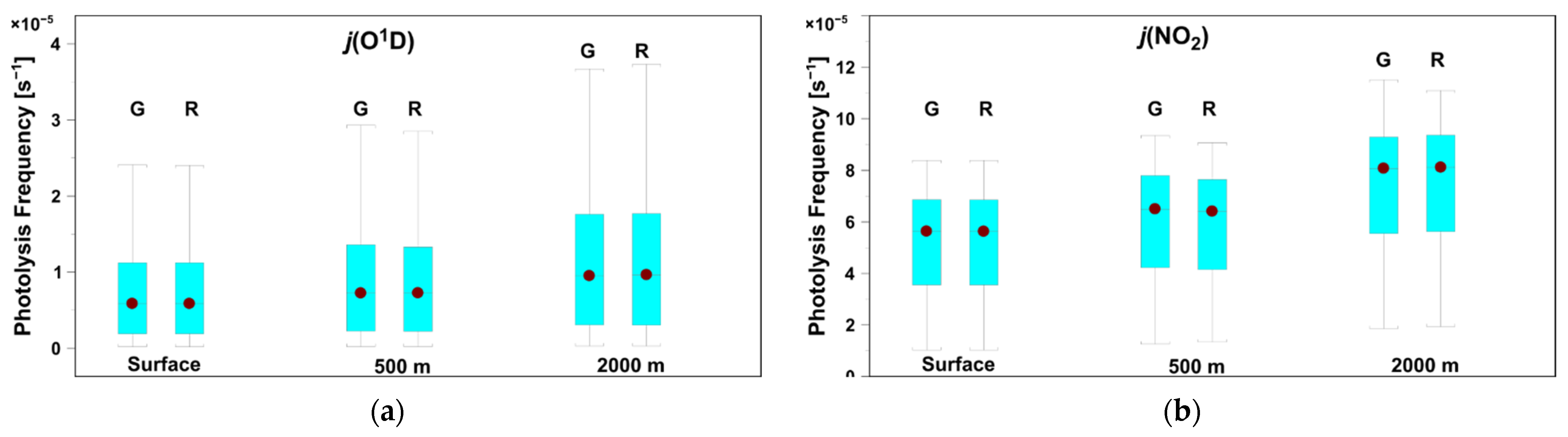
Level	Mean ± SD	Median	Percentile Range [2.5th:97.5th]	Minimum	Maximum
j (O1D)—GRASP
surface	0.724 × 10−5 ± 0.600 × 10−5	0.575 × 10−5	0.655 × 10−6:0.206 × 10−4	0.190 × 10−6	0.240 × 10−4
surface + 0.5 km	0.860 × 10−5 ± 0.710 × 10−5	0.706 × 10−5	0.820 × 10−6:0.244 × 10−4	0.235 × 10−6	0.285 × 10−5
surface + 2.0 km	0.114 × 10−4 ± 0.916 × 10−5	0.961 × 10−5	0.115 × 10−5:0.315 × 10−4	0.320 × 10−4	0.315 × 10−4
j (O1D)—REFERENCE
surface	0.730 × 10−5 ± 0.613 × 10−5	0.612 × 10−5	0.648 × 10−6:0.209 × 10−4	0.192 × 10−6	0.250 × 10−4
surface + 0.5 km	0.880 × 10−5 ± 0.729 × 10−5	0.749 × 10−5	0.816 × 10−6:0.248 × 10−4	0.229 × 10−6	0.296 × 10−4
surface + 2.0 km	0.113 × 10−4 ± 0.909 × 10−5	0.945 × 10−5	0.113 × 10−5:0.315 × 10−4	0.317 × 10−6	0.380 × 10−4
j (NO2)—GRASP
surface	0.519 × 10−2 ± 0.189 × 10−2	0.562 × 10−2	0.204 × 10−2:0.798 × 10−2	0.103 × 10−2	0.838 × 10−2
surface + 0.5 km	0.587 × 10−2 ± 0.202 × 10−2	0.637 × 10−2	0.238 × 10−2:0.876 × 10−2	0.134 × 10−2	0.907 × 10−2
surface + 2.0 km	0.750 × 10−2 ± 0.219 × 10−2	0.810 × 10−2	0.357 × 10−2:0.105 × 10−1	0.194 × 10−2	0.111 × 10−1
j (NO2)—REFERENCE
surface	0.520 × 10−2 ± 0.196 × 10−2	0.561 × 10−2	0.196 × 10−2:0.814 × 10−2	0.102 × 10−2	0.833 × 10−2
surface + 0.5 km	0.600 × 10−2 ± 0.209 × 10−2	0.652 × 10−2	0.241 × 10−2:0.902 × 10−2	0.126 × 10−2	0.922 × 10−2
surface + 2.0 km	0.746 × 10−2 ± 0.222 × 10−2	0.813 × 10−2	0.347 × 10−2:0.105 × 10−1	0.185 × 10−2	0.106 × 10−1

shows the statistical characteristics for j (O¹D) and j (NO₂) values obtained using the GRASP and the REFERENCE model. Despite the completely different inputs to the TUV model, there were only small differences between j values at each altitude level, up to a few percent. Photolysis frequencies increased with altitude, i.e., the mean values were ~55% (57% for GRASP and 55% for REFERENCE) and ~45% (45% for GRASP and 43% for REFERENCE) larger at the highest level comparing to those at the surface level for j (O¹D) and j (NO₂), respectively. Standard deviations also increased significantly with height, i.e., ~50% and 15%, respectively. The ratio of standard deviation to the mean value, the so-called coefficient of variation, was higher for j (O¹D) (~0.80) than that for j (NO₂) (~0.35). For the REFERENCE input, the coefficient of variation decreased with altitude, i.e., its change in a 2 km thick layer was from 0.84 to 0.80 (for j O¹D) and from 0.38 to 0.30 (for j (NO₂). Similar results were obtained using GRASP input, i.e., from 0.83 to 0.80 and from 0.36 to 0.30, respectively.

Further in the text, the statistics of the relative differences, denoted as Δ, between the j values obtained with different TUV inputs will be analyzed against the values obtained using the STANDARD model. Figure 7 shows the statistical properties of the relative differences for the fallowing pairs: REFERENCE versus STANDARD, GRASP versus STANDARD, and GRASP/MERRA versus STANDARD. To quantify the aerosols’ impact on j values, the relative differences between the TUV simulations with different input configurations were compared (

Table 3. Relative differences between j values obtained for various TUV input configurations in percentage of the j values obtained using the STANDARD input.

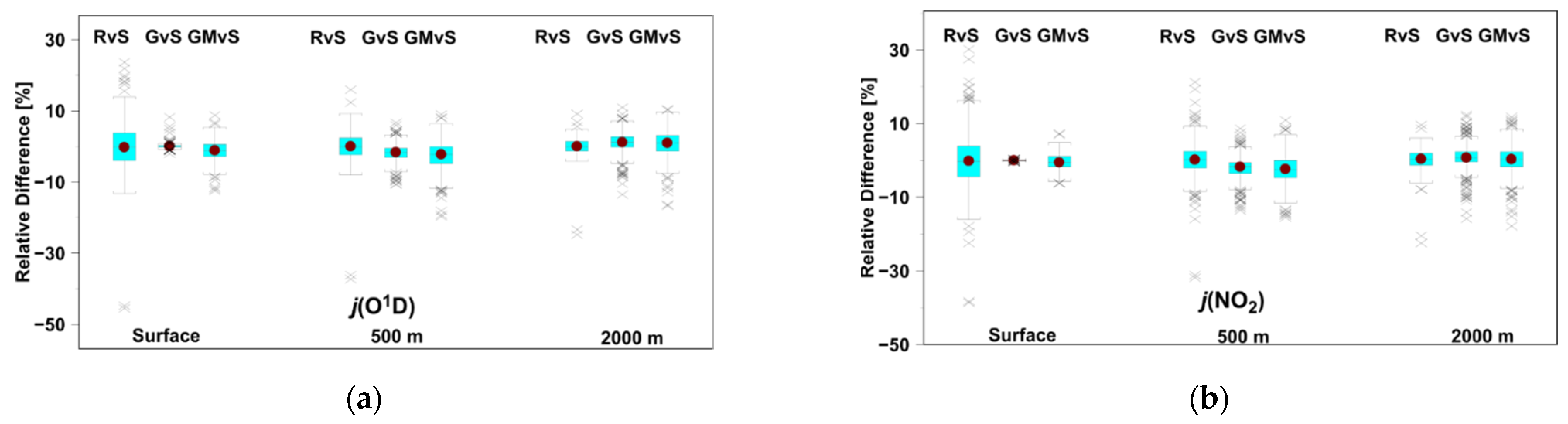
Level	Mean ± SD	Median	Percentile Range [2.5th:97.5th]	Minimum	Maximum
Δ[j (O1D)]: REFERENCE versus STANDARD
surface	0.06 ± 6.70	−0.25	−9.95:12.06	−45.48	23.65
surface + 0.5 km	0.00 ± 4.19	0.00	−5.88:6.94	−37.28	15.97
surface + 2.0 km	−0.03 ± 2.50	0.00	−3.31:3.74	−24.80	9.15
Δ[j (O1D)]: GRASP versus STANDARD
surface	0.08 ± 0.71	0.04	−1.00:1.02	−2.04	8.23
surface + 0.5 km	−1.89 ± 2.58	−1.68	−8.13:3.09	−10.7	6.70
surface + 2.0 km	1.17 ± 2.97	1.13	−7.25:6.61	−13.5	11.0
Δ[j (O1D)]: GRASP/MERRA versus STANDARD
surface	−1.21 ± 2.77	−1.16	−7.10:3.81	−12.4	8.75
surface + 0.5 km	−2.62 ± 4.05	−2.26	−12.2:4.44	−19.7	9.00
surface + 2.0 km	0.78 ± 3.68	0.97	−7.28:7.36	−16.7	10.5
Δ[j (NO2)]: REFERENCE versus STANDARD
surface	−0.04 ± 7.79	−0.18	−14.26:16.59	−38.64	33.39
surface + 0.5 km	−0.03 ± 4.78	0.16	−9.25:9.19	−31.85	21.27
surface + 2.0 km	0.16 ± 2.81	0.33	−4.72:4.49	−22.49	9.61
Δ[j (NO2)]: GRASP versus STANDARD
surface	−0.03 ± 0.11	−0.02	−0.29:0.18	−0.48	0.41
surface + 0.5 km	−2.16 ± 3.02	−1.79	−9.68:4.28	−13.6	8.6
surface + 2.0 km	0.84 ± 3.39	0.70	−8.42:7.91	−15.9	12.4
Δ[j (NO2)]: GRASP/MERRA versus STANDARD
surface	−0.38 ± 2.07	−0.59	−4.38:3.63	−6.26	7.25
surface + 0.5 km	−2.51 ± 3.80	−2.40	−11.4:4.40	−15.5	10.9
surface + 2.0 km	0.23 ± 3.81	0.27	−8.38:8.07	−17.8	11.8

). The relative differences are given in % of j values calculated with the TUV model with STANDARD input. The results for the TUV input pair, REFERENCE versus STANDARD, provide the benchmark values for other comparisons. Inter- and intraday changes of columnar AOC are included in the TUV model with the STANDARD input assuming Elterman’s α-profile. For other TUV model input pairs, “real” α-profiles were used for the comparison with the Elterman’s α-profile (default in STANDARD input), but they were constrained by the same AOD value from CIMEL observations. In addition, for the GRASP/MERRA input, SSA and ÅE changes with altitude were taken from MERRA-2 simulations.

Statistics of the relative differences between REFERENCE and STANDARD input in the TUV model show that changes in columnar AOCs forced especially large j variability at the surface relative to the case with fixed AOCs, i.e., the standard deviation of the pertaining relative differences was of ~7–8% and the 2.5th–97.5th percentile span of ~25% (~22% and 30% for j (O¹D) and j (NO₂), respectively). The extremes could reach −40% (for the minima) and 20–30% (for the maxima). Standard deviation of the relative differences decreased with the height. At the highest level (2 km above the surface), it was 2.5–2.8%, i.e., 2.5 times smaller than at the surface. The decrease with height was also found for the 2.5th–97.5th percentile range, i.e., ~12% and ~20% at 0.5 km above surface and ~7% and ~9% at 2 km for j (O¹D) and j (NO₂), respectively. Therefore, the range of the 2.5th–97.5th percentile narrowed down to about a third of that in the 2 km layer. The extreme values also decreased with height, and at the level of 2 km above surface, they amounted to about −20% (for the minima) and 10% (for the maxima).

The relative differences in j values obtained for the remaining TUV input pairs, GRASP versus STANDARD and GRASP/MERRA versus STANDARD, showed different patterns. Here, standard deviation of the relative differences was the smallest at the surface level and much less than the corresponding benchmark value. However, the relative differences increased with altitude. At the 2 km level, standard deviation (~3–4%) and the 2.5th–97.5th percentile range (~15%) became larger compared to the benchmark values for this level. The maxima at 2 km level above the surface were also comparable, but the minima were less negative by about 10 percentage points. In the comparison, GRASP/MERRA (variable SSA and ÅE in vertical profile) versus STANDARD input, the relative differences were slightly larger relative to those obtained in GRASP versus STANDARD input. This increase was more apparent for j values at the ground level.

Table 4. Cases with maximum negative relative difference between the TUV model with GRASP (or GRASP/MERRA) input and that using STANDARD input in percent of the j values by the TUV model with STANDARD input. SZA—solar zenith angle, O₃—total column ozone column in Dobson unit, TMP—temperature in °C, AOD—aerosol optical depth at 340 nm, SSA—single scattering albedo at 440 nm, AF—asymmetry factor at 440 nm, ÅE—Ångström exponent for the 340–440 nm range, Δ—the relative difference (in %) between j values from the TUV model comparison.

Level	Date (UTC) yy mm dd hh mm	SZA deg	O3 DU	TMP °C	AOD	SSA	AF	ÅE	Δ %
Δ[ j (O1D)]: GRASP versus STANDARD
Surf.	18 08 29 16 11	77.0	303	22.5	0.66	0.96	0.67	0.62	−2.0
Surf. + 0.5 km	18 08 29 16 11	77.0	303	21.4	0.66	0.96	0.67	0.62	−10.7
Surf. + 2.0 km	18 04 12 06 27	67.0	348	3.3	0.50	0.93	0.71	1.22	−13.5
Δ[ j (O1D)]: GRASP/MERRA versus STANDARD
Surf.	18 08 29 16 11	77.0	303	22.5	0.66	0.96	0.67	0.62	−12.4
Surf. + 0.5 km	18 08 29 16 11	77.0	303	21.4	0.66	0.96	0.67	0.62	−19.7
Surf. + 2.0 km	18 08 29 16 11	77.0	303	6.0	0.66	0.96	0.67	0.62	−16.7
Δ[ j (NO2)]: GRASP versus STANDARD
Surf.	18 05 21 16 31	72.6	358	17.9	0.27	0.95	0.66	1.40	−0.5
Surf. + 0.5 km	18 08 04 05 04	75.2	291	23.3	0.62	0.96	0.73	1.27	−13.6
Surf. + 2.0 km	18 04 12 06 27	67.6	348	3.3	0.50	0.93	0.70	1.22	−15.9
Δ[ j (NO2)]: GRASP/MERRA versus STANDARD
Surf.	15 08 10 09 07	40.6	300	29.9	1.25	0.96	0.74	1.24	−6.6
Surf. + 0.5 km	18 08 29 16 11	77.0	303	21.4	0.66	0.96	0.67	0.62	−15.5
Surf. + 2.0 km	18 04 12 06 27	67.6	348	3.3	0.50	0.93	0.71	1.22	−17.8

and

Table 5. The same as Table 4 but for the extreme positive differences between j values by the TUV models.

Level	Date (UTC) yy mm dd hh mm	SZA deg	O3 DU	TMP °C	AOD	SSA	AF	ÅE	Δ %
Δ[ j (O1D)]: GRASP versus STANDARD
Surf.	20 03 28 15 18	72.5	402	14.3	0.55	0.90	0.68	1.25	8.2
Surf. + 0.5 km	20 01 25 11 14	69.2	284	−2.6	0.25	0.98	0.76	0.25	6.7
Surf. + 2.0 km	16 09 10 15 10	71.5	280	7.9	0.43	0.95	0.70	1.43	11.0
Δ[ j (O1D)]: GRASP/MERRA versus STANDARD
Surf.	20 03 28 15 18	72.5	402	14.3	0.55	0.90	0.68	1.25	8.8
Surf. + 0.5 km	18 11 17 13 38	80.4	320	−0.8	0.24	0.80	0.68	1.10	9.0
Surf. + 2.0 km	16 09 12 15 05	71.5	286	7.9	0.41	0.91	0.68	1.29	10.5
Δ[ j (NO2)]): GRASP versus STANDARD
Surf.	18 11 17 13 38	80.4	320	3.3	0.24	0.80	0.68	1.10	0.4
Surf. + 0.5 km	20 01 25 11 14	69.2	284	−2.6	0.25	0.98	0.76	0.25	8.6
Surf. + 2.0 km	16 09 10 15 10	71.5	280	7.9	0.43	0.95	0.70	1.43	12.4
Δ[ j (NO2)]: GRASP/MERRA versus STANDARD
Surf.	17 01 23 09 03	74.0	298	−2.7	0.14	0.76	0.76	0.94	7.3
Surf. + 0.5 km	18 11 17 13 38	80.4	320	−0.8	0.24	0.80	0.68	1.10	10.9
Surf. + 2.0 km	16 09 15 15 30	76.4	276	6.9	0.39	0.92	0.72	1.21	11.8

show the dates, TCO3, temperature, and columnar aerosol characteristics for cases with the extreme differences, i.e., the maximal negative (Table 4) and the maximal positive (Table 5) difference between j values by the TUV models. The maximal negative differences appeared in August and April, and the maximal positive in January, March, September, and November. For example, at the level of 0.5 km, the maximum positive (6.7%) and negative differences (−10.7%) between j values by TUV model with the GRASP versus STANDARD input were on 25 January 2020 11:14 and 29 August 2018 16:11, respectively. Figure 1, Figure 2 and Figure 3 present results for these cases.

The extreme values shown in Table 4 and Table 5 were due to a specific vertical AOC pattern rather than unusual column AOC values. Extreme column AOC values (shown in Table 1) rarely appeared in Table 4 and Table 5, i.e., AOD_340 nm of 1.25 on 10 August 2015 at the surface (Table 4), ÅE for 340–440 nm range of 0.25 on 25 January 2020 at 0.5 km level, and SSA at 440 nm of 0.76 on 23 January 2017 (Table 5) at the surface. Other AOCs were quite typical, i.e., beyond the 2.5–97.5% range, only on 29 August 2018 for an AOD of 0.66, and on 17 November 2018 for an SSA of 0.80. Cases with extreme columnar AOC values are not always associated with extreme variations in j values due to the vertical AOC profiling. Therefore, it is impossible to predict the extreme influence of the AOC profile on j values based on the specific configuration of the columnar AOC properties, solar elevation, total column ozone, and temperature.

The extreme negative differences found in the comparison between the GRASP/MERRA versus STANDARD input were more negative than those between the GRASP versus STANDARD input (Table 4). It suggests the impact of the vertical profile of SSA and ÅE on extremely low j values. However, this is not so clear in the case of the extremely positive differences (Table 5), as larger extremes did not occur at the 2.0 km level.

4. Summary and Conclusions

The effect of vertical AOC changes on photolysis frequencies for the photodissociation of O₃ and NO₂ was analyzed. The TUV model (the newest version 5.4) with different input settings was applied to estimate photolysis frequencies at the surface and 0.5 and 2 km above it. The last two levels roughly represent the height of the planetary boundary layer for the stable and convective thermodynamic conditions. In Raciborz, simultaneous measurements of columnar AOC by the CIMEL Sun photometer and α-profile by the CHM-15k “Nimbus” ceilometer for the period 2015–2020 provided input values to the TUV model. In addition, the vertical profiles of SSA and ÅE were available based on the MERRA-2 data interpolated to the site’s location. Here, we present only the results based on model simulations. The ground-level measurements of the actinic flux were not available at the site. Previous studies showed that the TUV model is able to simulate j (O¹D) and j (NO₂) at the ground level (see for example the comparison in Figure 5 by Wang et al. [7]).

Firstly, TUV simulations with standard input (Elterman’s α-profile constrained with the measured AOD, and columnar values in the vertical profile for other AOCs) were compared with the reference input with fixed columnar AOCs (the averaged values of the CIMEL data for the period 2015–2020). The differences between output of these models provided a benchmark for j changes due to aerosols, consisting of the following statistics of the relative differences: standard deviation, 2.5th−97.5th percentile range, and the extreme values (minimum and maximum). The benchmark set comprises statistics for a typical aerosol configuration, i.e., only columnar AOC values are available at the site and the aerosol effect on j values can be deduced by comparison with the climatological AOC. At the ground level for j (O¹D), standard deviation and the 2.5th and 97.5th percentiles were 6.7, −10% and 12%, respectively (Table 3). The corresponding values for j (NO₂) were 7.8, −14.3% and 16.6%, respectively. These estimates agree with ~10% effect of the atmospheric aerosols on the photolysis rates, which was previously mentioned for Europe [6,21].

Next, we searched for discrepancies between the j values comparing the TUV model including the “real” α-profile (derived from ceilometer soundings and GRASP software) with the standard TUV input setting. In addition, we also examined the statistics of the differences (relative to j values by the standard TUV model) for the TUV model including the “real” α-profile and the MERRA-2 vertical profiles of SSA and ÅE.

Comparison of output of the STANDARD model with the model accounting for vertical changes in the AOCs (GRASP and GRASP/MERRA) allows the estimation of the effects caused by vertical changes in AOCs. Above the surface, the boxes and whiskers, shown in Figure 7 for the GRASP versus STANDARD and GRASP/MERRA versus STANDARD input pair, were comparable with those obtained for REFERENCE versus STANDARD (the benchmark set) input. This illustrates that the vertical profiling of AOCs causes variations in j values on a scale similar to that due to columnar AOC changes.

The benchmark values decreased with altitude. On the contrary, the increase of the statistical characteristics of the relative differences was found from the comparison between the TUV model with the “real” α-profile (instead of default Elterman’s profile) and the standard TUV model. At level 2 km above the surface, the variability caused by the “real” α-profile was even larger than the corresponding benchmark values. For example, relative differences for j (O¹D) were, 3.0, −7.3% and 6.6% versus benchmark values of 2.5, −3.3% and 3.7% for the standard deviation, 2.5th and 97.5th percentile, respectively. The corresponding ranges between the 2.5th and 97.5th percentile were 13.9% and 7%, respectively. This gives almost a two times larger span for the cases using the “real” α-profile. Such an increase was also found for j (NO₂). Case studies with the extreme values also suggested that the source of the extremes was the specific vertical variations of the AOCs.

To conclude, above the surface (at the 0.5 and 2 km levels), the vertical properties of aerosols significantly affected the distribution of the photolysis frequencies, i.e., on a similar scale to that due to variations in columnar AOCs (mostly AOD). This indicates that more detailed information about the vertical structure of aerosols is needed for credible atmospheric chemistry modeling. It is expected that space-borne LIDARs, planned to be used in ACE (The Aerosol–Cloud–Ecosystems) and EarthCARE (Earth Clouds, Aerosols, and Radiation Explorer) satellite missions, will provide such data.

References

- Kanakidou, M.; Crutzen, P.J. The photochemical source of carbon monoxide: Importance, uncertainties and feedbacks. Chemosph. Glob. Chang. Sci. 1999, 1, 91–109. [Google Scholar] [CrossRef]
- Finlayson-Pitts, B.J.; Pitts, J.N. Photochemistry of Important Atmospheric Species. Chem. Up. Low. Atmos. 2000, 4, 86–129. [Google Scholar] [CrossRef]
- Manisalidis, I.; Stavropoulou, E.; Stavropoulos, A.; Bezirtzoglou, E. Environmental and Health Impacts of Air Pollution: A Review. Front. Public Health 2020, 8, 14. [Google Scholar] [CrossRef] [Green Version]
- Shetter, R.E.; Müller, M. Photolysis frequency measurements using actinic flux spectroradiometry during the PEM-Tropics mission: Instrumentation description and some results. J. Geophys. Res. Atmos. 1999, 104, 5647–5661. [Google Scholar] [CrossRef]
- Webb, A.R.; Bais, A.F.; Blumthaler, M.; Gobbi, G.P.; Kylling, A.; Schmitt, R.; Thiel, S.; Barnaba, F.; Danielsen, T.; Junkermann, W.; et al. Measuring spectral actinic flux and irradiance: Experimental results from. J. Atmos. Ocean. Technol. 2002, 19, 1049–1062. [Google Scholar] [CrossRef]
- Gerasopoulos, E.; Kazadzis, S.; Vrekoussis, M.; Kouvarakis, G.; Liakakou, E.; Kouremeti, N.; Giannadaki, D.; Kanakidou, M.; Bohn, B.; Mihalopoulos, N. Factors affecting O3 and NO2 photolysis frequencies measured in the eastern Mediterranean during the five-year period 2002–2006. J. Geophys. Res. Atmos. 2012, 117, 22305. [Google Scholar] [CrossRef] [Green Version]
- Wang, W.; Li, X.; Shao, M.; Hu, M.; Zeng, L.; Wu, Y.; Tan, T. The impact of aerosols on photolysis frequencies and ozone production in Beijing during the 4-year period 2012–2015. Atmos. Chem. Phys. 2019, 19, 9413–9429. [Google Scholar] [CrossRef] [Green Version]
- Hofzumahaus, A.; Kraus, A.; Kylling, A.; Zerefos, C.S. Solar actinic radiation (280–420 nm) in the cloud-free troposphere between ground and 12 km altitude: Measurements and model results. J. Geophys. Res. Atmos. 2002, 107, PAU 6-1–PAU 6-11. [Google Scholar] [CrossRef]
- Kylling, A. Fast simulation tool for ultraviolet radiation at the earth’s surface. Opt. Eng. 2005, 44, 41012. [Google Scholar] [CrossRef]
- Mayer, B.; Kylling, A. Technical note: The libRadtran software package for radiative transfer calculations-Description and examples of use. Atmos. Chem. Phys. 2005, 5, 1855–1877. [Google Scholar] [CrossRef] [Green Version]
- Madronich, S. The Atmosphere and UV-B Radiation at Ground Level. In Environmental UV Photobiology; Springer: Boston, MA, USA, 1993; pp. 1–39. [Google Scholar] [CrossRef]
- Shettle, E.P. Models of aerosols, clouds and precipitation for atmospheric propagation studies. In Proceedings of the AGARD Conference, Copenhagen, Denmark, 1989; Volume 454, pp. 1–13. [Google Scholar]
- Elterman, L. UV, visible and IR attenuation for alititudes to 50 km. Environ. Res. Paper 1968, 285, 49. [Google Scholar]
- Sukhodolov, T.; Rozanov, E.; Ball, W.T.; Bais, A.; Tourpali, K.; Shapiro, A.I.; Telford, P.; Smyshlyaev, S.; Fomin, B.; Sander, R.; et al. Evaluation of simulated photolysis rates and their response to solar irradiance variability. J. Geophys. Res. Atmos. 2016, 121, 6066–6084. [Google Scholar] [CrossRef] [Green Version]
- Molero, F.; Fernández, A.J.; Revuelta, M.A.; Martínez-Marco, I.; Pujadas, M.; Artíñano, B. Effect of Vertical Profile of Aerosols on the Local Shortwave Radiative Forcing Estimation. Atmosphere 2021, 12, 187. [Google Scholar] [CrossRef]
- Tie, X.; Madronich, S.; Walters, S.; Zhang, R.; Rasch, P.; Collins, W. Effect of clouds on photolysis and oxidants in the troposphere. J. Geophys. Res. Atmos. 2003, 108, D20. [Google Scholar] [CrossRef]
- Hall, S.R.; Ullmann, K.; Prather, M.J.; Flynn, C.M.; Murray, L.T.; Fiore, A.M.; Correa, G.; Strode, S.A.; Steenrod, S.D.; Lamarque, J.F.; et al. Cloud impacts on photochemistry: Building a climatology of photolysis rates from the Atmospheric Tomography mission. Atmos. Chem. Phys. 2018, 18, 16809–16828. [Google Scholar] [CrossRef] [Green Version]
- Fountoulakis, I.; Natsis, A.; Siomos, N.; Drosoglou, T.; Bais, A.F. Deriving aerosol absorption properties from solar ultraviolet radiation spectral measurements at Thessaloniki, Greece. Remote Sens. 2019, 11, 2179. [Google Scholar] [CrossRef] [Green Version]
- Markowicz, K.M.; Flatau, P.J.; Kardas, A.E.; Remiszewska, J.; Telmaszczyk, K.; Woeste, L. Ceilometer retrieval of the boundary layer vertical aerosol extinction structure. J. Atmos. Ocean. Technol. 2008, 25, 928–944. [Google Scholar] [CrossRef]
- Li, J.; Wang, Z.; Wang, X.; Yamaji, K.; Takigawa, M.; Kanaya, Y.; Pochanart, P.; Liu, Y.; Irie, H.; Hu, B.; et al. Impacts of aerosols on summertime tropospheric photolysis frequencies and photochemistry over Central Eastern China. Atmos. Environ. 2011, 45, 1817–1829. [Google Scholar] [CrossRef]
- Real, E.; Sartelet, K. Modeling of photolysis rates over Europe: Impact on chemical gaseous species and aerosols. Atmos. Chem. Phys. 2011, 11, 1711–1727. [Google Scholar] [CrossRef] [Green Version]
- Péré, J.C.; Bessagnet, B.; Pont, V.; Mallet, M.; Minvielle, F. Influence of the aerosol solar extinction on photochemistry during the 2010 Russian wildfires episode. Atmos. Chem. Phys. 2015, 15, 10983–10998. [Google Scholar] [CrossRef] [Green Version]
- Ruggaber, A.; Dlugi, R.; Nakajima, T. Modelling radiation quantities and photolysis frequencies in the troposphere. J. Atmos. Chem. 1994, 18, 171–210. [Google Scholar] [CrossRef]
- Liao, H.; Yung, Y.L.; Seinfeld, J.H. Effects of aerosols on tropospheric photolysis rates in clear and cloudy atmospheres. J. Geophys. Res. Atmos. 1999, 104, 23697–23707. [Google Scholar] [CrossRef] [Green Version]
- Kylling, A.; Webb, A.R.; Bais, A.F.; Blumthaler, M.; Schmitt, R.; Thiel, S.; Kazantzidis, A.; Kift, R.; Misslbeck, M.; Schallhart, B.; et al. Actinic flux determination from measurements of irradiance. J. Geophys. Res. Atmos. 2003, 108, 4506. [Google Scholar] [CrossRef]
- Ångström, A. On the Atmospheric Transmission of Sun Radiation and on Dust in the Air. Geogr. Ann. 1929, 11, 156–166. [Google Scholar] [CrossRef]
- Dickerson, R.R.; Kondragunta, S.; Stenchikov, G.; Civerolo, K.L.; Doddridge, B.G.; Holben, B.N. The impact of aerosols on solar ultraviolet radiation and photochemical smog. Science 1997, 278, 827–830. [Google Scholar] [CrossRef] [Green Version]
- Holben, B.N.; Eck, T.F.; Slutsker, I.; Tanré, D.; Buis, J.P.; Setzer, A.; Vermote, E.; Reagan, J.A.; Kaufman, Y.J.; Nakajima, T.; et al. AERONET-A federated instrument network and data archive for aerosol characterization. Remote Sens. Environ. 1998, 66, 1–16. [Google Scholar] [CrossRef]
- Błaszczak, B.; Zioła, N.; Mathews, B.; Klejnowski, K.; Słaby, K. The Role of PM2.5 Chemical Composition and Meteorology during High Pollution Periods at a Suburban Background Station in Southern Poland. Aerosol Air Qual. Res. 2020, 20, 2433–2447. [Google Scholar] [CrossRef]
- Szkop, A.; Pietruczuk, A. Analysis of aerosol transport over southern Poland in August 2015 based on a synergy of remote sensing and backward trajectory techniques. J. Appl. Remote Sens. 2017, 11, 016039. [Google Scholar] [CrossRef] [Green Version]
- Szkop, A.; Pietruczuk, A. Synergy of satellite-based aerosol optical thickness analysis and trajectory statistics for determination of aerosol source regions. Int. J. Remote Sens. 2019, 40, 8450–8464. [Google Scholar] [CrossRef]
- Goloub, P.; Li, Z.; Dubovik, O.; Blarel, L.; Podvin, T.; Jankowiak, I.; Lecoq, R.; Deroo, C.; Chatenet, B.; Morel, J.P.; et al. In Proceedings of the PHOTONS/AERONET Sunphotometer Network Overview: Description, Activities, Results, Orlando, FL, USA, 22 April 2008. [CrossRef] [Green Version]
- Sinyuk, A.; Holben, B.N.; Eck, T.F.; Giles, D.M.; Slutsker, I.; Korkin, S. The AERONET Version 3 aerosol retrieval algorithm, associated uncertainties and comparisons to Version 2. Atmos. Meas. Tech. 2020, 13, 3375–3411. [Google Scholar] [CrossRef]
- AERONET Data Download Tool. Available online: https://aeronet.gsfc.nasa.gov/cgi-bin/webtool_inv_v3 (accessed on 15 December 2021).
- AERONET Data Download Tool. Available online: https://aeronet.gsfc.nasa.gov/cgi-bin/webtool_aod_v3 (accessed on 15 December 2021).
- Valenzuela, A.; Olmo, F.J.; Lyamani, H.; Antón, M.; Titos, G.; Cazorla, A.; Alados-Arboledas, L. Aerosol scattering and absorption Angström exponents as indicators of dust and dust-free days over Granada (Spain). Atmos. Res. 2015, 154, 1–13. [Google Scholar] [CrossRef] [Green Version]
- Fernandes, A.; Pietruczuk, A.; Szkop, A.; Krzyścin, J. Aerosol Layering in the Free Troposphere over the Industrial City of Raciborz in Southwest Poland and Its Influence on Surface UV Radiation. Atmosphere 2021, 12, 812. [Google Scholar] [CrossRef]
- CHM 15k Datasheet. Available online: http://cedadocs.ceda.ac.uk/1243/1/CHM15k_Datasheet.pdf (accessed on 15 December 2021).
- Wiegner, M.; Geiß, A. Aerosol profiling with the Jenoptik ceilometer CHM15kx. Atmos. Meas. Tech. 2012, 5, 1953–1964. [Google Scholar] [CrossRef] [Green Version]
- Dubovik, O.; Herman, M.; Holdak, A.; Lapyonok, T.; Tanré, D.; Deuzé, J.L.; Ducos, F.; Sinyuk, A.; Lopatin, A. Statistically optimized inversion algorithm for enhanced retrieval of aerosol properties from spectral multi-angle polarimetric satellite observations. Atmos. Meas. Tech. 2011, 4, 975–1018. [Google Scholar] [CrossRef] [Green Version]
- Dubovik, O.; Lapyonok, T.; Litvinov, P.; Herman, M.; Fuertes, D.; Ducos, F.; Torres, B.; Derimian, Y.; Huang, X.; Lopatin, A.; et al. GRASP: A versatile algorithm for characterizing the atmosphere. In SPIE Newsroom; Society of Photo-Optical Instrumentation Engineers: Bellingham, WA, USA, 2014; p. 4. [Google Scholar]
- Ou, Y.; Li, L.; Li, Z.; Zhang, Y.; Dubovik, O.; Derimian, Y.; Chen, C.; Fuertes, D.; Xie, Y.; Lopatin, A.; et al. Spatio-Temporal Variability of Aerosol Components, Their Optical and Microphysical Properties over North China during Winter Haze in 2012, as Derived from POLDER/PARASOL Satellite Observations. Remote Sens. 2021, 13, 2682. [Google Scholar] [CrossRef]
- Li, L.; Dubovik, O.; Derimian, Y.; Schuster, G.L.; Lapyonok, T.; Litvinov, P.; Ducos, F.; Fuertes, D.; Chen, C.; Li, Z.; et al. Retrieval of aerosol components directly from satellite and ground-based measurements. Atmos. Chem. Phys. 2019, 19, 13409–13443. [Google Scholar] [CrossRef] [Green Version]
- Lopatin, A.; Dubovik, O.; Chaikovsky, A.; Goloub, P.; Lapyonok, T.; Tanré, D.; Litvinov, P. Enhancement of aerosol characterization using synergy of lidar and sun-photometer coincident observations: The GARRLiC algorithm. Atmos. Meas. Tech. 2013, 6, 2065–2088. [Google Scholar] [CrossRef] [Green Version]
- Lopatin, A.; Dubovik, O.; Fuertes, D.; Stenchikov, G.; Lapyonok, T.; Veselovskii, I.; Wienhold, F.G.; Shevchenko, I.; Hu, Q.; Parajuli, S. Synergy processing of diverse ground-based remote sensing and in situ data using the GRASP algorithm: Applications to radiometer, lidar and radiosonde observations. Atmos. Meas. Tech. 2021, 14, 2575–2614. [Google Scholar] [CrossRef]
- Román, R.; Benavent-Oltra, J.A.; Casquero-Vera, J.A.; Lopatin, A.; Cazorla, A.; Lyamani, H.; Denjean, C.; Fuertes, D.; Pérez-Ramírez, D.; Torres, B.; et al. Retrieval of aerosol profiles combining sunphotometer and ceilometer measurements in GRASP code. Atmos. Res. 2018, 204, 161–177. [Google Scholar] [CrossRef] [Green Version]
- Titos, G.; Ealo, M.; Román, R.; Cazorla, A.; Sola, Y.; Dubovik, O.; Alastuey, A.; Pandolfi, M. Retrieval of aerosol properties from ceilometer and photometer measurements: Long-term evaluation with in situ data and statistical analysis at Montsec (southern Pyrenees). Atmos. Meas. Tech. 2019, 12, 3255–3267. [Google Scholar] [CrossRef] [Green Version]
- Gelaro, R.; McCarty, W.; Suárez, M.J.; Todling, R.; Molod, A.; Takacs, L.; Randles, C.A.; Darmenov, A.; Bosilovich, M.G.; Reichle, R.; et al. The modern-era retrospective analysis for research and applications, version 2 (MERRA-2). J. Clim. 2017, 30, 5419–5454. [Google Scholar] [CrossRef] [PubMed]
- Chin, M.; Ginoux, P.; Kinne, S.; Torres, O.; Holben, B.N.; Duncan, B.N.; Martin, R.V.; Logan, J.A.; Higurashi, A.; Nakajima, T. Tropospheric aerosol optical thickness from the GOCART model and comparisons with satellite and sun photometer measurements. J. Atmos. Sci. 2002, 59, 461–483. [Google Scholar] [CrossRef]
- Colarco, P.; Da Silva, A.; Chin, M.; Diehl, T. Online simulations of global aerosol distributions in the NASA GEOS-4 model and comparisons to satellite and ground-based aerosol optical depth. J. Geophys. Res. Atmos. 2010, 115, 14207. [Google Scholar] [CrossRef] [Green Version]
- Buchard, V.; Randles, C.A.; da Silva, A.M.; Darmenov, A.; Colarco, P.R.; Govindaraju, R.; Ferrare, R.; Hair, J.; Beyersdorf, A.J.; Ziemba, L.D.; et al. The MERRA-2 aerosol reanalysis, 1980 onward. Part II: Evaluation and case studies. J. Clim. 2017, 30, 6851–6872. [Google Scholar] [CrossRef]
- Randles, C.A.; da Silva, A.M.; Buchard, V.; Colarco, P.R.; Darmenov, A.; Govindaraju, R.; Smirnov, A.; Holben, B.; Ferrare, R.; Hair, J.; et al. The MERRA-2 aerosol reanalysis, 1980 onward. Part I: System description and data assimilation evaluation. J. Clim. 2017, 30, 6823–6850. [Google Scholar] [CrossRef]
- Colarco, P.R.; Nowottnick, E.P.; Randles, C.A.; Yi, B.; Yang, P.; Kim, K.M.; Smith, J.A.; Bardeen, C.G. Impact of radiatively interactive dust aerosols in the NASA GEOS-5 climate model: Sensitivity to dust particle shape and refractive index. J. Geophys. Res. Atmos. 2014, 119, 753–786. [Google Scholar] [CrossRef]
- Meng, Z.; Yang, P.; Kattawar, G.W.; Bi, L.; Liou, K.N.; Laszlo, I. Single-scattering properties of tri-axial ellipsoidal mineral dust aerosols: A database for application to radiative transfer calculations. J. Aerosol Sci. 2010, 41, 501–512. [Google Scholar] [CrossRef]
- Hess, M.; Koepke, P.; Schult, I. Optical Properties of Aerosols and Clouds: The Software Package OPAC. Bull. Am. Meteorol. Soc. 1998, 79, 831–844. [Google Scholar] [CrossRef]
- Bohren, C.F.; Huffman, D.R. Absorption and Scattering of Light by Small Particles; John Wiley: New York, NY, USA, 1993. [Google Scholar] [CrossRef] [Green Version]
- Global Modeling and Assimilation Office (GMAO). MERRA-2 inst3_3d_aer_Nv: 3d,3-Hourly,Instantaneous,Model-Level,Assimilation,Aerosol Mixing Ratio V5.12.4; Goddard Earth Sciences Data and Information Services Center (GES DISC): Greenbelt, MD, USA, 2015. Available online: https://disc.gsfc.nasa.gov/datasets/M2I3NVAER_5.12.4/summary (accessed on 15 December 2021).
- Global Modeling and Assimilation Office (GMAO). MERRA-2 inst3_3d_asm_Np: 3d,3-Hourly,Instantaneous,Pressure-Level,Assimilation,Assimilated Meteorological Fields V5.12.4; Goddard Earth Sciences Data and Information Services Cente: Greenbelt, MD, USA, 2015. Available online: https://disc.gsfc.nasa.gov/datasets/M2I3NPASM_5.12.4/summary (accessed on 15 December 2021).
- Tropospheric Ultraviolet and Visible (TUV) Radiation Model|Atmospheric Chemistry Observations & Modeling (ACOM). Available online: https://www2.acom.ucar.edu/modeling/tropospheric-ultraviolet-and-visible-tuv-radiation-model (accessed on 15 December 2021).
- Madronich, S. Photodissociation in the atmosphere: 1. Actinic flux and the effects of ground reflections and clouds. J. Geophys. Res. Atmos. 1987, 92, 9740–9752. [Google Scholar] [CrossRef]