Evaluation of Forward Models for GNSS Radio Occultation Data Processing and Assimilation

Abstract

In radio occultation (RO) data processing and data assimilation, the forward model (FM) is used to calculate bending angle (BA) from refractivity (N). The accuracy and precision of forward modeled BA are affected by refractivity profiles and FM methods, including Abel integral algorithms (direct, exp, exp_T, linear) and methods of interpolating refractivity during integral (log-cubic spline and log-linear). Experiment 1 compares these forward model methods by comparing the difference and relative difference (RD) of the experimental value (forward modeled ECMWF analysis) and the true value (BA of FY3D RO data). Results suggested that the exp with log-cubic spline (log-cubic) interpolation is the most accurate FM because it has better integral accuracy (less than 2%) to inputs, especially when the input is lower than an order of magnitude of 1 × 10⁻² (that is, above 60 km). By contrast, the direct induced a 10% error, and the improvement of exp T to exp is limited. Experiment 2 simulated the exact errors of an FM (exp) based on inputs on different vertical resolutions. The inputs are refractivity profiles on model levels of three widely used analyses, including ECMWF 4Dvar analysis, final operational global analysis data (FNL), and ERA5. Results demonstrated that based on exp and log-cubic interpolation, BA on model level of ECMWF 4Dvar has the highest accuracy, whose RD is 0.5% between 0–35 km, 4% between 35–58 km, and 1.8% between 58–80 km. By contrast, the other two analyses have low accuracy. This paper paves the way to better understanding the FM, and simulation errors on model levels of three analyses can be a helpful FM error reference.

1. Introduction

The global navigation satellite system (GNSS) radio occultation (RO) technique has many advantages: high vertical resolution, global coverage, and long-term steady data. It has been proven that RO can significantly improve the accuracy of numerical weather prediction (NWP) after being assimilated into the NWP assimilation system. According to [1], RO observation ranked fourth among data that affected NWP. With the rapid development of the RO technique, numerous missions have been planned, launched, and run steadily to serve the operational NWP, such as Constellation Observing System for Meteorology, Ionosphere, and Climate (COSMIC/COSMIC-2), the Meteorological Operational satellite Programme-A/B (MetOpA/B), FengYun-3C/D (FY-3C/D) [2], GRACE/GRACE-FO, Scientific Application Satellite-C/D (SAC-C/D), Korea Multi-Purpose Satellite-5 (KOMPSAT-5), and Spanish PAZ (‘peace’ in Spanish) [3,4,5]. By 2027, these missions will provide approximately 18,400 observations per day which theoretically is the number threshold of the positive effect that RO could bring to NWP [6,7]. It will reduce error in prediction by 25% if all these observations are assimilated into the NWP assimilation system [8]. However, the actual situation does not coincide with theoretical expectations because almost half of the RO data either cannot be received or cannot pass quality control before assimilation [9]. There are two strategies to increase the RO observation available. The first one focus on increasing the soundings received per day via more missions, more receivers on the cube satellite, e.g., the cube satellite constellation of Spire company [10], and more multi-system-compatible RO receiver such as GNSS Radio Occultation Sonder (GNOS) onboard FY3 [2,11,12,13]. The second strategy is to improve the RO data processing technique. The current RO data processing center includes the Danish Meteorological Institute (DMI), German Research Centre for Geosciences (GFZ), Jet Propulsion Laboratory (JPL), University Corporation for Atmospheric Research (UCAR), the National Oceanic and Atmospheric Administration (NOAA) ’s National Environmental Satellite, Data, and Information Service (NESDIS), and Wegener Center/the University of Graz (WEGC). Each center developed different schemes to process RO data. The quality of their RO data is accessed by the international RO working group (IROWG) every other year [14]. The consistency and structural uncertainty of their RO data records are promising to step up to another level. Thus, improvements are expected in the RO data processing and RO data assimilation techniques. The forward model (FM) plays a critical role during these two processes. Firstly, the more accurate the FM, the more accurate these two processes. Secondly, the error of FM should be quantified, so that the other errors during these two processings can be accurately evaluated. The FM mainly consists of Abel integral algorithm and interpolation methods before Abel integral.

1.1. FM Algorithm in Data Assimilation and RO Data Processing

(1) FM in RO data assimilation. In terms of the RO data assimilation, two options, the bending angle (BA) or refractivity, are used for variational assimilation [15,16]. The option of forward modeled BA is convenient and concise. During assimilation, atmospheric parameters are firstly transformed to refractivity (N)

$$N=77.6\frac{p}{T}+3.73\times {10}^5\frac{e}{T^2}$$

(1)

where T is temperature, e is water vapor partial pressure, and p is pressure. Then the refractivity is inverted to BA ($\alpha$) by the Abel integral, a core part of FM

$$\alpha (a)=-2a{\displaystyle {\int }_a^{\infty }\frac{d\ln (n)}{dx}}\frac{dx}{\sqrt{x^2-a^2}}$$

(2)

where a is impact parameter, refractive index n = 10⁻⁶N + 1. Hence, the accuracy of BA is strongly affected by n and the FM. This BA is then assimilated into the NWP data assimilation system. Therefore, the FM is critical for RO data assimilation.

(2) FM in RO data processing. The FM is employed to correct the ionospheric error to BA during RO data processing by the method of statistical optimization. The ionosphere frequently interferes with GPS signals [17]. There are several approaches for ionospheric calibration: the linear combination of two frequencies corrects the first order; the K-correction corrects the higher-order [18]; the statistical optimization corrects all the ionospheric error [19]. The last one is based on background climatological models such as MSIS-90 (mass spectrometer and incoherent scatter radar in 1990) [20], BAROCLIM (the bending angle radio occultation climatology) based on Formosat-3/COSMIC data [21], and CIRA (the 1986 COSPAR International Reference Atmosphere) [21]. Most data in these background climatological models are stored as refractivity. Therefore, we need to invert them to BA via FM. Therefore, the accuracy of the FM is important.

In another aspect, the RO data are also used in commercial companies or civilian industries, wherein they might consider using some analysis data sets to assimilate RO data in their assimilation systems or develop their own RO data processing program. Generally, widely used and free analysis data sets are considered. However, some of those data sets have limited vertical and horizontal resolution. Therefore, how many biases the forward modeling results contain is open to debate. The biases are generated by not only forward models but also the level resolution of the analysis data. Therefore, the level resolution of the original data should also be under consideration for evaluating the error of FMs.

1.2. FM Algorithm

The core of an FM is the Abel integral, whose original form is given by Equation (2), in which two singularities exist: $x=a$ and $x=\infty$. To solve such problem, [22] used hyperbolic transformation and an algorithm that closely resembles the Abel integral was obtained, which we call the direct algorithm in this study.

To further improve the approximation accuracy, the interpolation and numerical approximation methods were employed. For example, based on the physical assumption of isothermal atmosphere and temperature exponential approximation with height, refractivity was assumed to decrease exponentially with impact parameters. Methods of exponential extrapolation and interpolation of refractivity were summarized by the European Center for Medium-Range Weather Forecasts (ECMWF) [23,24,25]. In such a method, numerical approximation, such as the error function (erf), was also employed. This method is called the exp algorithm in this paper. Subsequently, the linear assumption of the BA was considered in the Abel integral inversion, called the linear algorithm in this paper. Both exp and linear algorithms are incorporated in the radio occultation processing package (ROPP) software developed by the Radio Occultation Meteorology Satellite Application Facility [24,26]. Later, it was found that oscillations occur between levels (vertical grids) of the forward modeled BA using the exp algorithm. In order to correct this oscillation, [24] revised the exp algorithm by adopting more temperature operators in the refractivity operator; the modified algorithm is called the exp_T algorithm in this paper. For more details on these four algorithms, refer to Appendix A: Abel Integral Algorithms. In addition to the four methods, the NOAA National Centers for Environmental Prediction (NCEP) used quadratic Lagrangian polynomials [27], which avoided the exponential decay of refractivity with height.

The FM is the integral algorithm as shown in Equation (2), in which the refractivity was firstly interpolated along a denser grid of impact parameter to improve integration accuracy. Therefore, the accuracy of an FM is closely associated with the interpolation method and numerical integral method. In terms of interpolation methods, authors of [28] found that the log-cubic spline (hereafter, log-cubic) is the most accurate one. Log-cubic interpolation projects refractivity into the log space and then interpolates it by the log-cubic method. In addition to this interpolation method, log-linear interpolation is tested in this paper. To the best of our limited knowledge, most studies either focus on the numerical integration method or only on the interpolation methods.

Thus far, a systematic discussion on the combination of interpolation and integration methods has not been reported. In addition, to the best of our knowledge, only a few results have been reported on the estimation of the error of the FM occurring on a fixed model level, for example 137 EC. The present study aims to discuss both of these aspects.

In this study, first, we compare three Abel integral algorithms, namely direct, exp, and exp_T algorithms, and two interpolation methods, namely log-cubic and log-linear. Second, we evaluate errors of FMs on the model levels of three analyses. To achieve these two aims, we set two experiments. In experiment 1, we compare FMs and interpolation methods. In experiment 2, the most accurate FM is employed to calculate the BA on model levels of three widely used analysis datasets, namely ECMWF 4Dvar analysis with 137 levels, ECMWF ERA5 analysis with 37 levels, and final operational global analysis data (FNL) with 31 levels. Furthermore, the errors of FMs are simulated, providing an error reference for FMs under the analyzed model levels. The simulation also demonstrates to what extent a low-resolution model level can be used for conducting comparative research of RO products. Our research provides a better understanding of the error of FMs in RO data processing and assimilation. In the experiments conducted in this study, a point-to-point comparison is made horizontally. It should be noted that we ignore the tangent point drift (that is the practical RO profiles are slanting rather than being vertical to the ground, which may result in the refractivity gradient bias [27]), since the interval of each level is less than 10 km [28].

This paper is organized as follows. The principles of the four algorithms in the forward model are described in Section 1. In Section 2, the progress of experiments 1 and 2 are introduced, together with data selection and low-pass filter strategies. Results are presented in Section 3. Finally, we discuss and present the discussion and conclusion in Section 4.

2. Experiments

In this study, two experiments were conducted. The first experiment compared the algorithms together with interpolation methods. Subsequently, the most accurate integral and interpolation method was used in the second experiment, in which the refractivity profiles on levels of widely used analyses—FNL, EC4Dvar, and ERA5—were calculated to the BA by FMs. Then, the bias of results was evaluated.

2.1. Data, Collocation, and Quality Control

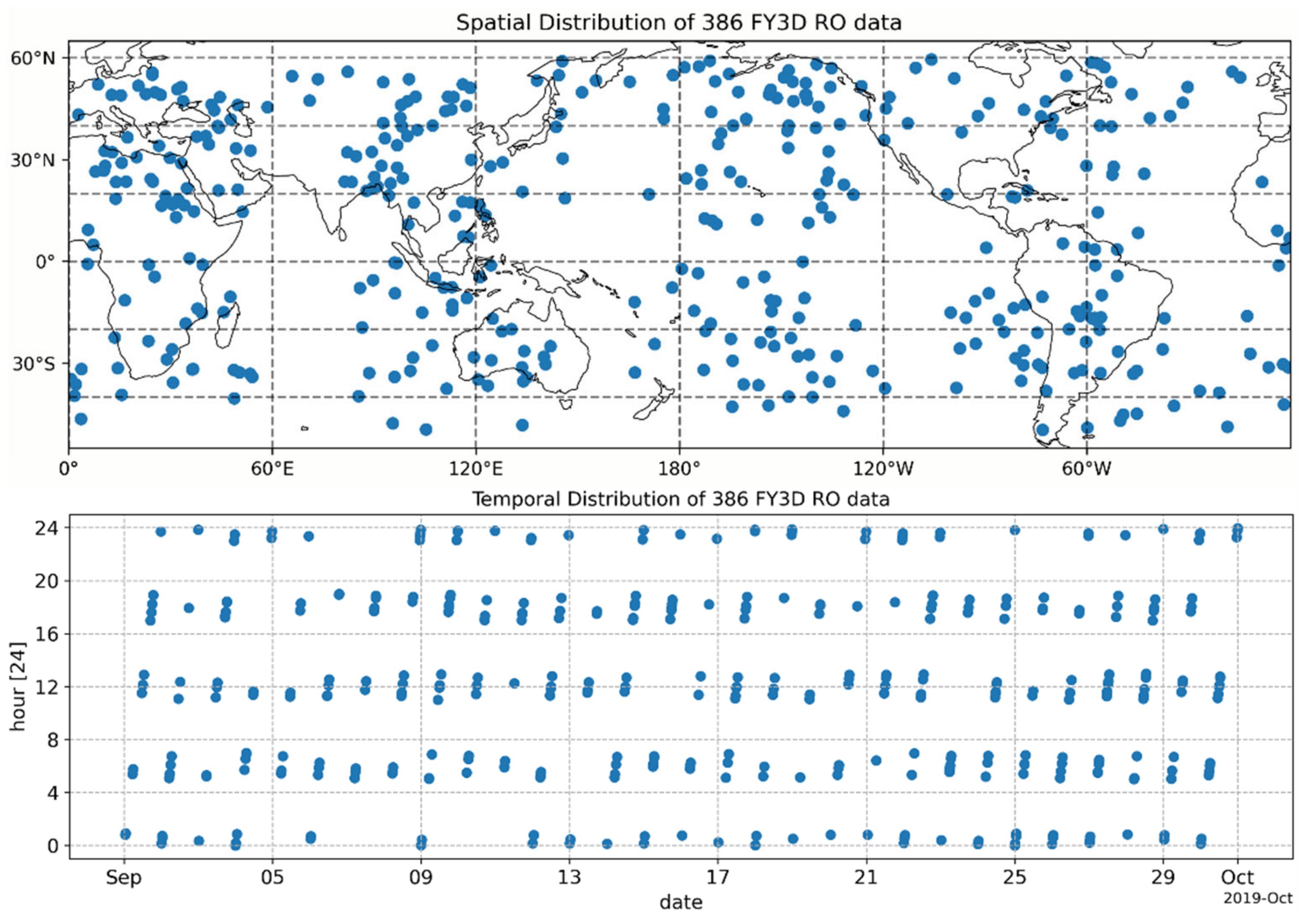
2.1.1. Data

We used the FY3D observation in September 2019 as the ‘true value’ which is available for download at http://www.nsmc.org.cn (accessed on 8 June 2021). The daily number of occultation soundings is approximately 500, and the vertical resolution is approximately 150–300 m. The quality control of the FY3D data is assessed by the China Meteorological Administration [29], and the result has been qualified by ECMWF [5]. The qualiy control result is displayed in near real-time (NRT) monitoring at the ROM SAF website (Available at: https://www.romsaf.org/monitoring/index.php (accessed on 8 June 2021)). As shown in Figure A2 in Appendix B, the quality of FY3D (The mean relative difference (RD) between ECMWF forecast and FY3D is less than 2%) in September 2019 established a good condition for experiment 1.

We also used ECMWF operational analyses in experiment 1, which can be accessed at https://www.ecmwf.int/en/forecasts/dataset/operational-archive (accessed on 8 June 2021). Such data are produced daily by ECMWF’s direct 4Dvar atmospheric model. Hereafter we call this data EC4Dvar. These data are in 128 × 64 grids; hence, the resolution is approximately 2.8° × 2.8°; They have 137 levels and are output daily at four hours: 00, 06, 12, and 18 UTC. Since the resolution of EC4Dvar is very coarse, we used strict collocation and quality control.

In experiment 1, the refractivity profiles were the experimental values; Therefore, we first calculated refractivity from temperature, water vapor partial pressure, and pressure of EC4Dvar via Equation (1) according to their own level grids.

In experiment 2, we used FY3D to simulate analyses such as ECMWF, ERA5, and FNL. The level of them are 137, 37, and 31 respectively. The height and levels interval can be found Figure A3 in Appendix B.

2.1.2. Spatial and Temporal Collocation

Experiment 1 aims to compare the BA from FY3D retrievals and calculated using Equation (2) from EC4Dvar atmospheric profiles. To improve the accuracy of the comparison, we must ensure that the refractivity profiles of EC4Dvar and FY3D are collocated.

In terms of temporal collocation, we only selected the occultation soundings whose time is less than one hour to EC4Dvar’s four main synoptic hours, namely 00, 06, 12, and 18 UTC; that is, $\left|T_{FY3D}-T_{EC4D\mathrm{var}}\right|\le 1$ h. 5914 out of 17791 FY3D GNOS soundings in September 2019 satisfied the temporal collocation.

In terms of spatial collocation, we used the tangent point of occultation profiles as its location to search its nearest EC4Dvar profile. The profile with 137 levels on grids nearest to the tangent point was selected. In such a way, we assume the EC4Dvar and the FY3D profiles are collocated. However, because a grid resolution of 2.8° × 2.8° is too large, the collocated profiles of EC4Dvar may be far be far FY3D. We fixed it in quality control as explained in the next subsection. Figure A7 in Appendix C shows that FY3D soundings in experiment 1 generally have an evenly spatial and temporal distribution, which makes the mean (statistical values) feasible in the subsequent analysis.

2.1.3. Quality Control

Since we used coarse resolution EC4Dvar to collocate with FY3D data, some FY3D’s collocated profile may be far from it. To ensure that the refractivity of FY3D is close to that of ECMWF and to make sure the results have statistical representativeness, we set four steps of quality control (hereafter 4QC). These four steps were initially a scheme for quality control used by [30] to compare MetOp RO data from two different RO data processing centers, which is concise and effective [31]. The details of 4QC can be found in Appendix C. After 4QC, 368 out of 5914 FY3D soundings remained for experiment 1. The high rate of discard is attributed to the low resolution (2.8° × 2.8°) EC4Dvar.

In experiment 1, EC4Dvar’s refractivity was transformed to BA. The forward-modeled BA contained not only the bias introduced by FMs and interpolations but also the inherent bias of the inputs when they were refractivity. Experiment 2 was a simulation experiment, in which only FY3D was used. Therefore, the data quality was not taken into consideration.

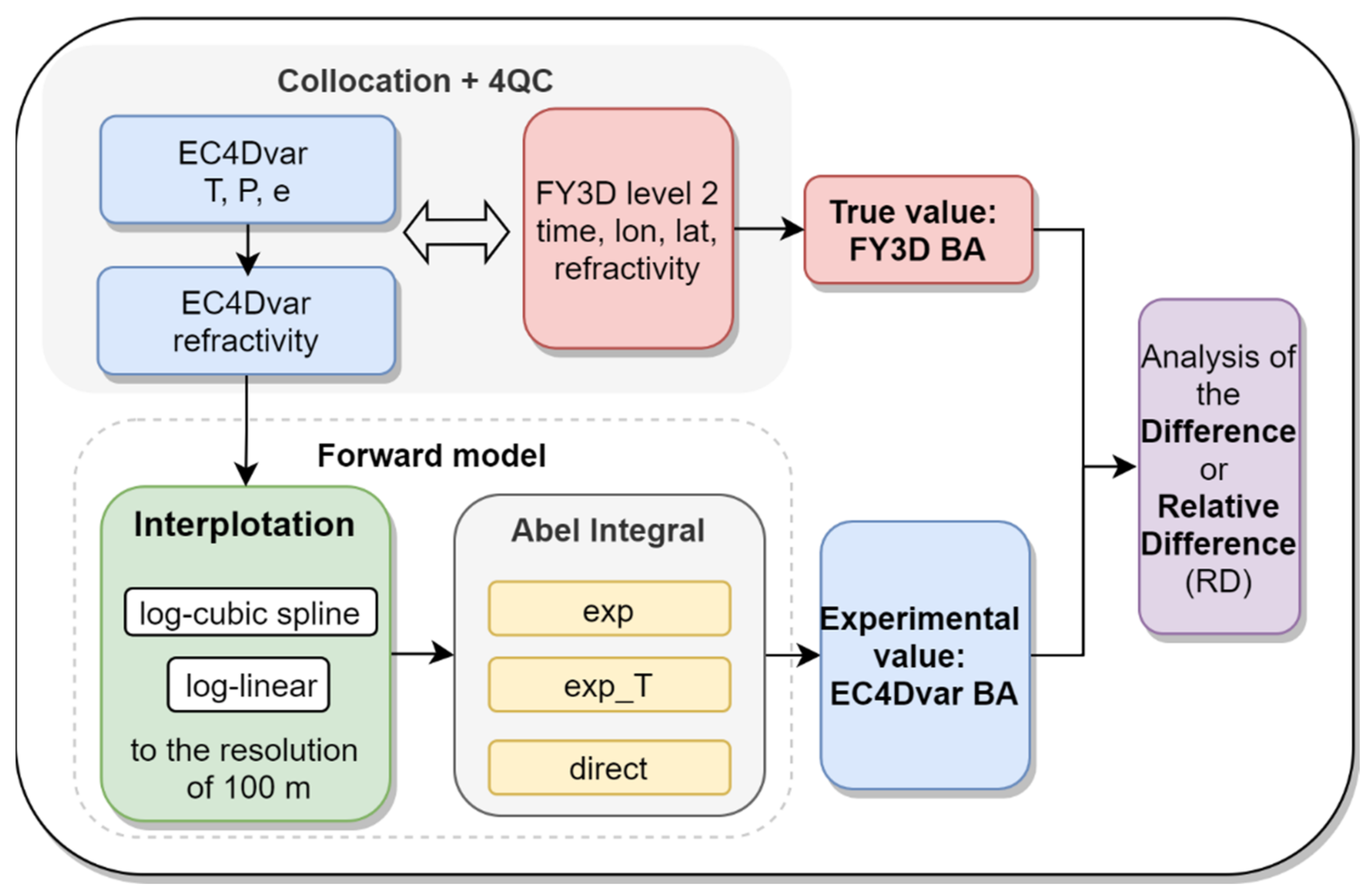
2.2. Experiment 1: Algorithm Comparison

Experiment 1 aims to determine the most accurate FM by comparing FM algorithms that considered interpolation methods.

There are three types of bias in RO data processing: observation errors, ionospheric errors, and errors incurred within the data processing. We focused on the third error in experiment 1, mainly the bias from the Abel numerical integral and interpolation methods. The Abel integral methods considered in this experiment were the direct, exp, and exp_T algorithms. The interpolation methods were log-cubic and log-linear, indicated in the subsequent figures by no label and “lin”, respectively. The log-cubic maps refractivity into the log space and then interpolates it by the cubic spline method; the log-linear also projects refractivity into the log space, but interpolates it in a linear fashion.

In this experiment, 368 FY3D BA profiles in September 2019 were regarded as the true value (T). The collocated refractivity profiles of EC4Dvar were the experimental value (E), which were calculated via Equation (1) on the data’s inherent 137 levels. The temporal and spatial collocation of both sets of data is described in Section 2.1., as well as the further 4QCs for collocation. From the statistical perspective, we used the mean to analyze the results, which would not be affected by outliers s. Two statistics were selected for the analysis: the difference of the BA, i.e., (E − T); and the relative difference (RD) of the BA, i.e., ((E − T)/T × 100%). Based on these statistics, we determine how close an FM’s result is to the true value; Another form of RD, which is the difference between two experimental values, i.e., ((E₁ − E₂)/E₂ × 100%), can avoid introducing the bias of true value and provide the difference between the two experimental values. Subsequently, the relatively better FM can be obtained.

Figure 1 shows the process of experiment 1. (1) FY3D profiles collocated with the EC4Dvar atmospheric profiles with respect to time, longitude, and latitude. Subsequently, the EC4Dvar profiles of atmospheric parameters were transformed to refractivity profiles. Then, the 4QC was performed for FY3D and EC4Dvar. We regarded the 4QC-passed FY3D BA as the true value (T). (2) The EC4Dvar refractivity profiles on 137 levels were interpolated into a resolution of 100 m by the log-cubic space and log-linear methods. (3) The interpolated refractivity was then transformed into the BA by three different integral methods. (4) The forward-modeled EC4Dvar BA was regarded as the experimental value (E) and was compared with the FY3D BA in terms of the difference (E − T) and RD (E − T)/T $\times$ 100%. Note that the log-cubic interpolation was applied to the impact parameter instead of the mean sea level (MSL) height, since impact parameter x equals refractivity(n) multiple position vector (r). Because dn/dr is extremely large near a high-water-vapor region, which cannot satisfy the condition of applying cubic spline interpolation: the value to be interpolated should be continuously incremented.

It is noteworthy that the true value and experimental value are only an estimated value to their actual values. Therefore, the difference between any FM and FY3D, (E_FMx − T), is just an estimate showing which algorithm is closer to the truth. By contrast, the difference between any two FMs (E_FM1 − E_FM2) is the absolute difference value. Experiment one shows which FM is better, instead of expressing how much error is incurred from the FM. Through experiment 1, although we can determine which FM is better, how much error exactly is incurred from the FM cannot be expressed. Such a question can refer to experiment 2.

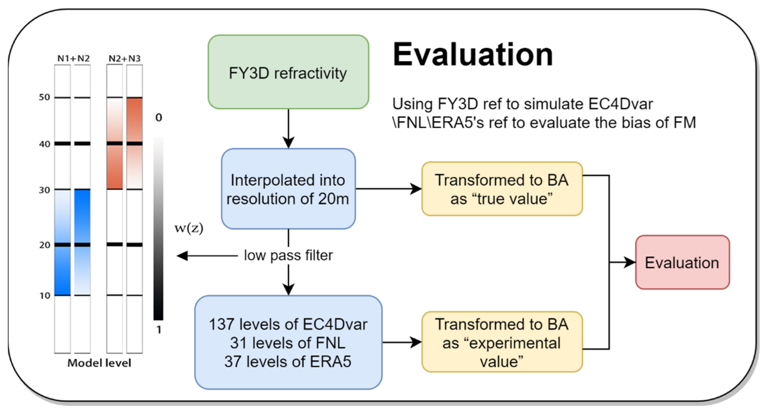
2.3. Experiment 2: Evaluation of Errors of FMs on the Fixed Model Level

Experiment 2 explores how much bias was introduced from transforming the analyses’ refractivity to the BA. As shown in Figure 2, FY3D refractivity profiles were first linearly interpolated into a resolution of 20 m and then transformed to the BA as the true value. These interpolated refractivity profiles were then filtered to remove the small-scale chaos less than the model grid interval of analyses such as 137 levels of ECMWF 4dvar, 31 levels of FNL, and 37 levels of ERA5 via the low pass filter. Their intervals are shown in Figure A3 source not found. in Appendix B. Subsequently, the refractivity profiles were linearly interpolated onto model grids and then transformed to the BA as the experimental value. Finally, obeying the nearest principle, the nearest true value level to the experimental value was selected to evaluate the experimental value. Note that the FM used in this experiment was the most accurate one with its experimental value being the nearest to the true value. In addition, considering computation efficiency [28], we chose two interpolation methods, namely log-spine cubic and log-linear.

Finally, the low pass filter must be mentioned here. Interpolation from a high resolution (20 m) to a low resolution (model levels) requires a filter, or it will induce representativeness errors [32]. For this purpose, we applied the Savitzky-Golay low-pass filter [33]. In general, the data are filtered with a window of $2\delta z$ or $4\delta z$ ($3\delta z$ typically results in instability [34]). In this study, $2\delta z$ is set. The next problem we encountered was that intervals of model levels increasing with height. To fix it, on the basis of [28], we divided the intervals into three groups: below the height of 0–20 km, 20–40 km, and above the height of 40–60 km. A window of twice the average interval of each group, 2$\delta {\overline{z}}_i$, was applied to filter the whole profile; thus, we had three filtered refractivity profiles, N1, N2, and N3. To merge them smoothly at the transition point (20 km and 40 km), we used a transition function, w(z), which is changed linearly from 1 to 0, as shown in the left subfigure in Figure 2. The refractivity profiles at the transition point are expressed as

$$\begin{array}{l}{N}_{10to30}=\frac{1}{2}\left[w_1(z)\times N_1+\left(1-w_2(z)\right)\times N_2\right]\\ N_{30to50}=\frac{1}{2}\left[w_2(z)\times N_2+\left(1-w_3(z)\right)\times N_3\right]\end{array}$$

(3)

where $w_i(z)$ is the transition function to $N_i$ (i = 1, 2, 3), and z is the height. $N_{0to10}$ and $N_{50to60}$ were filtered by the filter window themselves. The combination of those slices by height was the terminal profiles.

Furthermore, the following details were considered in this experiment. First, to improve simulation accuracy and reduce the interpolation error, we selected 20 m, instead of 100 m, as the resolution for FY3D to simulate the analysis. Second, the analysis model level was simulated, and those levels were transformed into MSL height for convenience. Third, the true value was refractivity instead of BA. The true value also passed the same Abel transform as the forward-modeled BA in the analysis.

3. Results

In this section, the results of experiment 1 are presented, which demonstrate the most accurate FM. Subsequently, two simulated errors of the most accurate FM are obtained on the basis of three widely used analyses: EC4Dvar, FNL, and ERA5.

3.1. Experiment 1: Algorithm Comparison

In this experiment, we compared three Abel integral algorithms and two interpolation methods. The BA of FY3D was the true value, while the forward-modeled EC4Dvar BA was the experimental value. The FY3D observation data were filtered by the strict collocation and 4QC strategies. Subsequently, 368 FY3D profiles in September 2019 remained, which were regarded as the true value (T). EC4Dvar refractivity data collocated with the true values were the experimental values (E). We used two statistics in this experiment: the difference (A $-$ B) and relative difference (A $-$ B)/B × 100%, where A and B can be either E and T or E and E, respectively. The obtained statistics were all mean values. Note that we compared the exp algorithm with the direct and exp_T algorithms independently because the exp_T algorithm is too close to the exp algorithm. If the exp_T algorithm was drawn in the same figure with the direct algorithm, it would coincide with the graph of the exp algorithm.

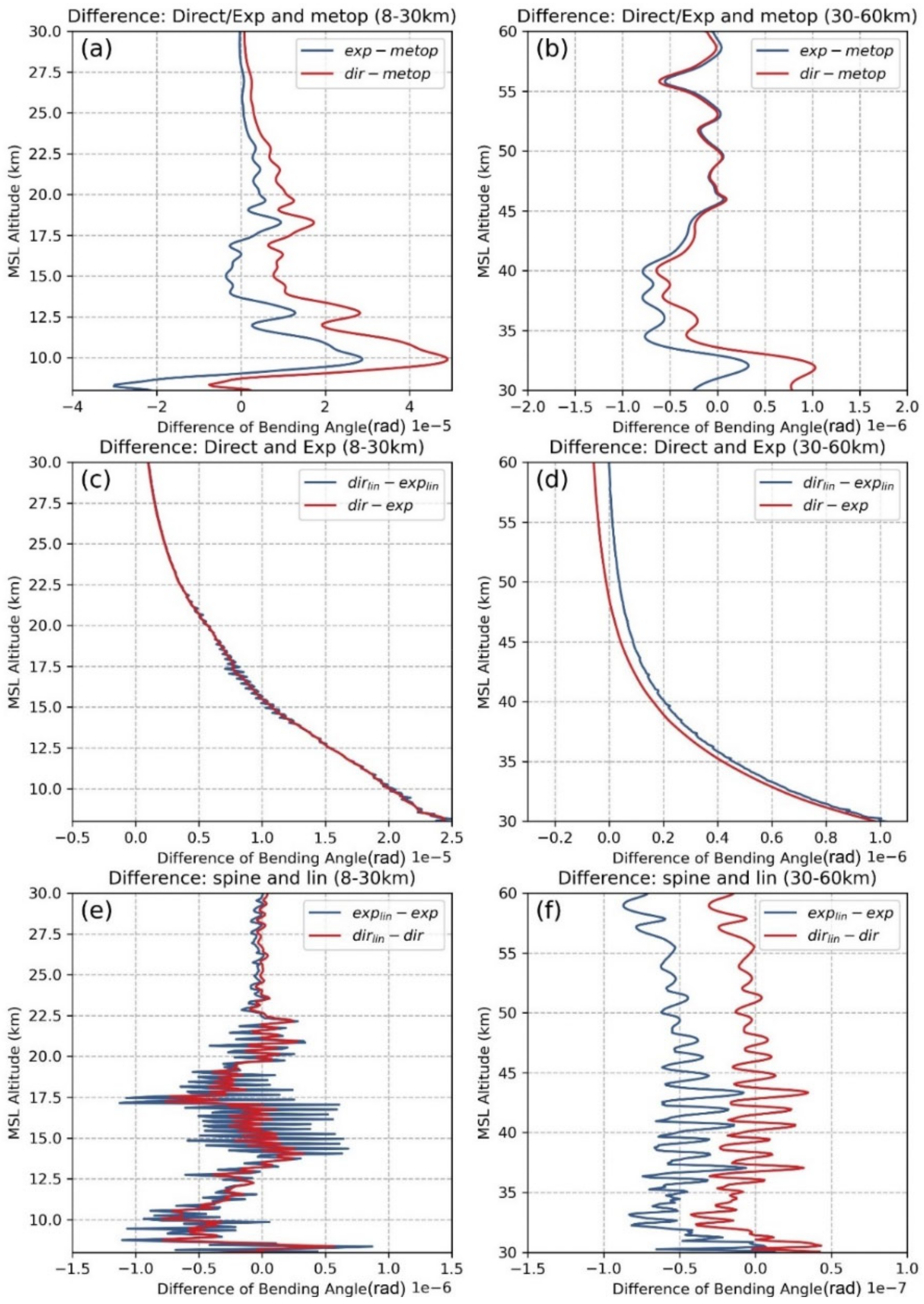
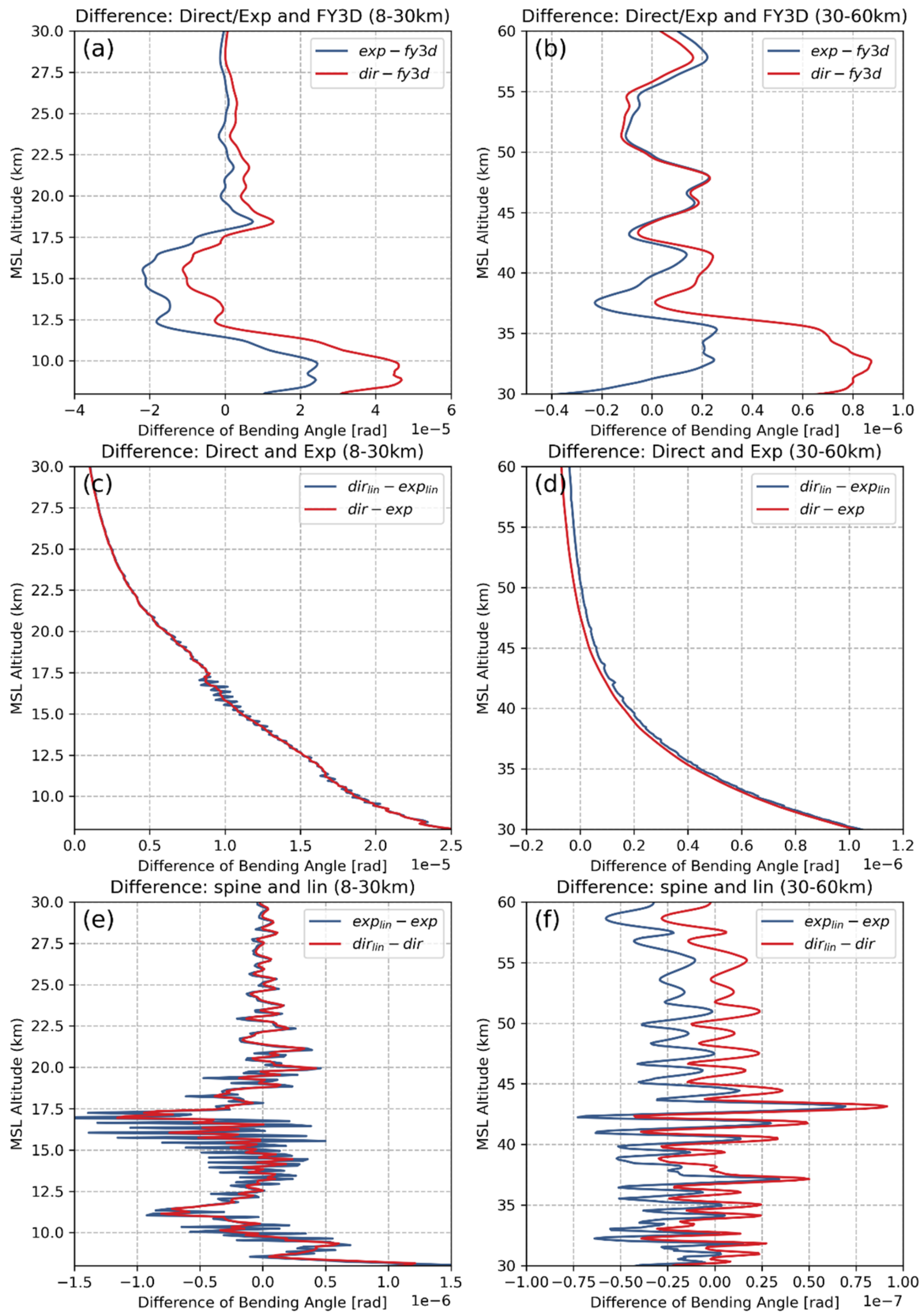
3.1.1. Difference Analysis for Direct and Exp

First, we compared the difference (E $-$ T), in which E is the BA integrated by the exp and direct Abel integral algorithms, together with two interpolation methods. The altitude starts from 5 km because the signal-to-noise ratio below it is low, and some RO observations are unavailable. As shown in Figure 3a,b, differences of both algorithms are in the same order of magnitude; 1 × 10⁻⁵ is within 5–30 km, and 1 × 10⁻⁶ is within 30–60 km. However, the exp is more accurate than the direct because it is closer to the true value except at heights of 12.5–17.5 km, which reflects the errors passed by refractivity. Figure 3c,d shows the difference between the two algorithms. The result of the direct is larger than that of the exp until at a height of 50 km. Figure 3e,f shows the difference due to interpolation. In the height range of 5–30 km, the error induced by log-linear is less than ±1 × 10⁻⁶, and above 30 km, it is less than ±0.5 × 10⁻⁷. Interestingly, log-linear interpolation causes more undulation compared with log-cubic interpolation. The undulation due to interpolation is larger for the exp algorithm. To verify this result, we repeated this experiment using MetOp as the true value, and the same conclusion was drawn (see Figure A4 in Appendix B).

3.1.2. Relative Difference Analysis of Direct and Exp Algorithms

Next, we analyzed the RD, (E $-$ T)/T × 100%, of the FY3D BA (T) and the forward modeled EC4Dvar BA (E) in different FMs and show the results in Figure 4a–c. The orders of magnitude of the differences in the ranges of 5–55 km, 55–70 km, and 70–80 km are within 1–1.5%, 4–−10%, and 10–80%, respectively. This result is consistent with those of the previous studies [28,35,36]. The results shown in Figure 4a–c are divided into three aspects for clarity. (i) The RD of the exp is near to zero than that of the direct, indicating the BA of the exp algorithm is closer to the true value. In other words, the exp algorithm is more accurate than the direct algorithm. The result of the direct algorithm is larger than the true value below 60 km (approximately 0.3% larger than exp) and considerably less than the true value above 60 km. (ii) Since these two algorithms have the same input and same vertical-level setting, this gap is probably due to the integral accuracy of the algorithm. The integral accuracy depends on the order of magnitude of refractivity (input), which is shown in Figure A5 in Appendix B. Intriguingly, when the order of magnitude is 1 × 10⁻² above (below) a height of 60 km, the direct algorithm’s result is less (larger) than the true value. (iii) Note that at heights of 18, 48, and 58 km, larger errors are incurred by refractivity rather than the errors of the FM. Unexpectedly, the errors of the exp algorithm at these heights are larger than those of the direct algorithm. This difference can be attributed to the fact that refractivity of the exp algorithm exponentially decays faster than that of the direct algorithm.

The green and blue lines in Figure 4d–f illustrate the RD between the direct and exp algorithms. Below 60 km, their difference is less than ±2%, whereas above 60 km, it is considerably large. The RDs between the two algorithms based on the two interpolation methods are indicated by the orange and pink lines; the RD is even larger when the algorithms are based on log-cubic interpolation. In general, the errors due to log-linear interpolation of the FM with the exp algorithm are larger than those with the direct algorithm. The RD of two interpolations with the exp algorithm is less than 0.2%, −2%, and −20% for heights of 5–50, 55–65, and 70–80 km, respectively. Specifically, because these errors are almost equal to the monthly errors of FY3D to ECMWF recorded in the ROM website (see Figure A2) the log-linear interpolation can be considered to be not sufficiently accurate. However, if such an error is acceptable, the exp algorithm with log-linear interpolation will be a timely and effective FM, since the log_linear interpolation is more cost-efficient than the log-cubic interpolation.

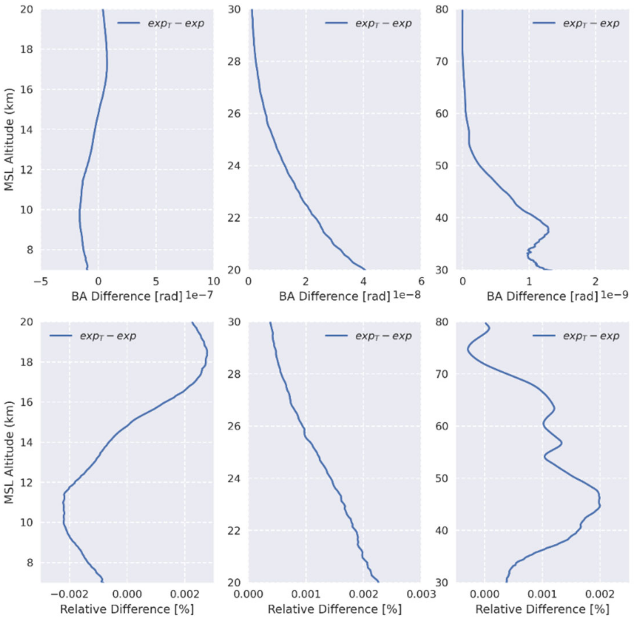
3.1.3. Analysis to exp_T

Herein, we discuss the RD and difference between the exp and the revised exp algorithm (exp_T). The RD is two orders of magnitude lower than the difference between exp and direct. Hence, the RD and difference are plotted in separate graphs as shown in Figure 5, the BA of the exp_T algorithm is slightly larger than that of the exp algorithm. According to [24], this difference is due to the temperature term in the new polynomial, which corrects the error of the exp algorithm. However, the corrected amount is limited. Since the exp_T algorithm introduced temperature operator, it requires considerably more computation and time resources. Thus, the exp algorithm is superior operationally.

Finally, we list the RD between the true value and all experimental values in

Table 1. Relative difference, (E−T)/T × 100%, between the FY3D BA (T) and the forward-modeled BA (E), in which E can be the exp and direct algorithm, and each algorithm has two interpolation methods: log linear (denoted by lin) and cubic spline (no label).

H (km)	exp (%)	exp_lin(%)	direct(%)	direct_lin(%)	exp_T(%)	exp_T_lin(%)
8–15	(−0.3, 0.5)		exp + 0.3		exp ± 0.002	exp_lin ± 0.002
15–20	(0.5, 1)		exp + 0.3
20–45	(−0.3, 0.5)		exp + 0.2
45–55	(−0.5, 1.5)		exp + 0.1
55–60	(0, 5)	(0, 4)	(0, 3.8)
60–70	(−1, 2.5)	(−4, 2.3)	(−10, 1.8)
70–80	(−1, 5)	(−20, −5)	(−80, −10)	direct + 4%

. The above analysis identified that the exp algorithm with log-cubic is the most accurate FM; therefore, the quantity of each FM’error is written as exp’s RD plus the left error of the FM for clarity. First, the RD of the exp_lin algorithm is the same as that of the exp algorithm below a height of 55 km; however, it becomes 3% and 20% larger than that of the exp algorithm within 55–60 km and 70–80 km, respectively. Second, the RD of the direct algorithm is approximately 0.3% larger than that of the exp algorithm within 8–45 km, which becomes −10% and −80% less than that of the exp algorithm within 60–70 km and 70–80 km, respectively. Third, the improvement of the exp_T algorithm is limited (approximately 0.002%) compared to that of the exp algorithm. It should be noted within heights of 55–60 km, the error of the exp_lin algorithm is less than that of the exp algorithm, which is due to errors contributed by refractivity.

The exp algorithm with log-cubic is the most accurate FM; therefore, the quantity of each FM’error is written as exp’s RD plus the left error of the FM for clarity.

It is important to note that when E was refractivity, there are already been errors in E_ref (ref is refractivity). This error was then passed to BA’s (E−T)/T. Therefore, what we got in experimentone is the which FM is better, rather than how much error exactly one FM causes. This issue will be tested in experiment two. Since analysis above identified that the exp algorithm with log-cubic interpolation is the most accurate FM, in next experiment we will figure out how much exactly the error of exp algorithm is on three fixed model levels.

It is important to note that when E is refractivity, errors exist in E_ref (where ref denotes refractivity), which are then passed to the (E−T)/T value of the BA. Therefore, experiment 1 demonstrates which FM is better, rather than how much error exactly an FM causes, which will be tested in experiment 2. The above analysis indicated that the exp algorithm with log-cubic interpolation is the most accurate FM; therefore, in experiment 2, we determined the extent of error of the exp algorithm on three fixed model levels.

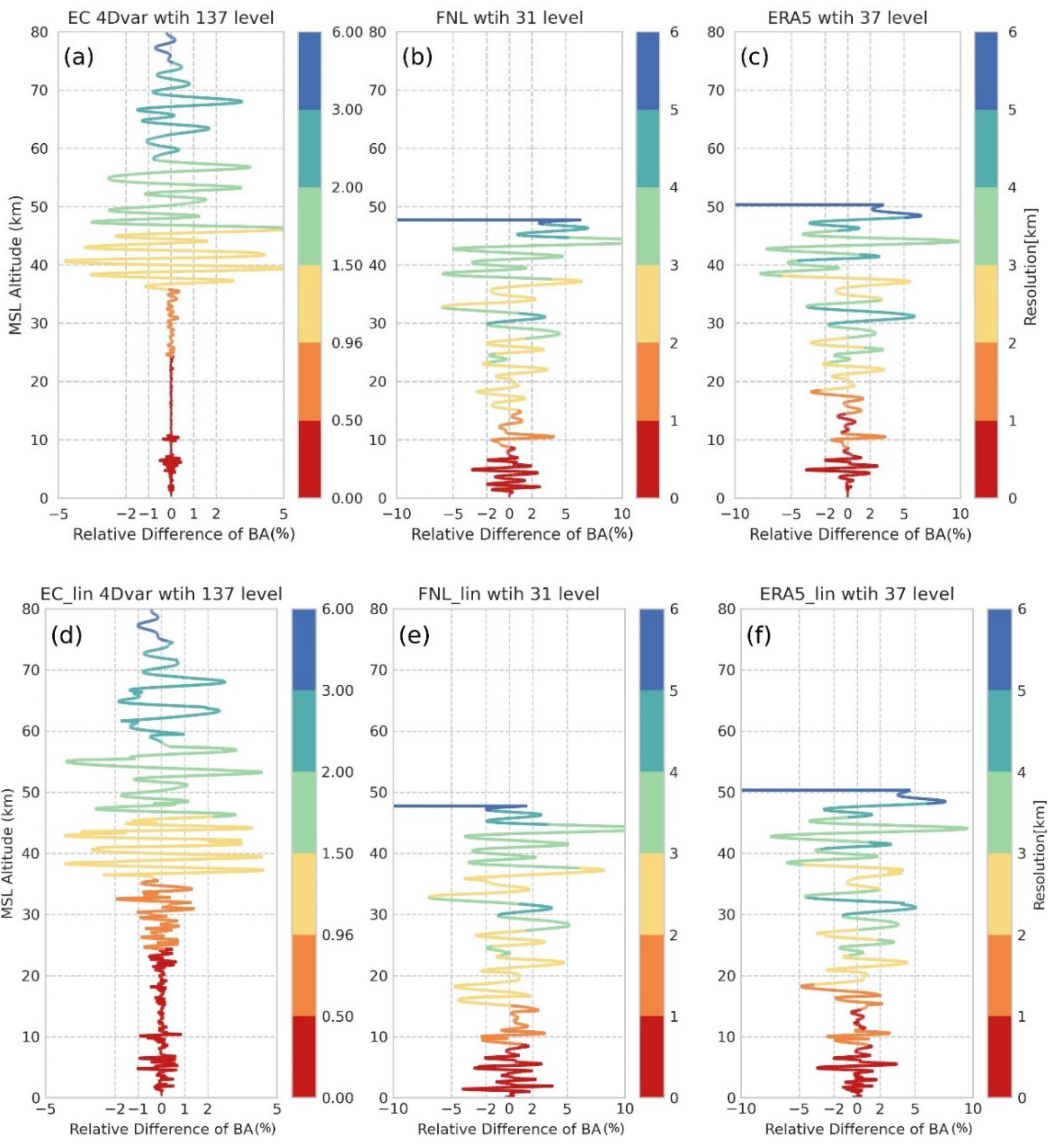
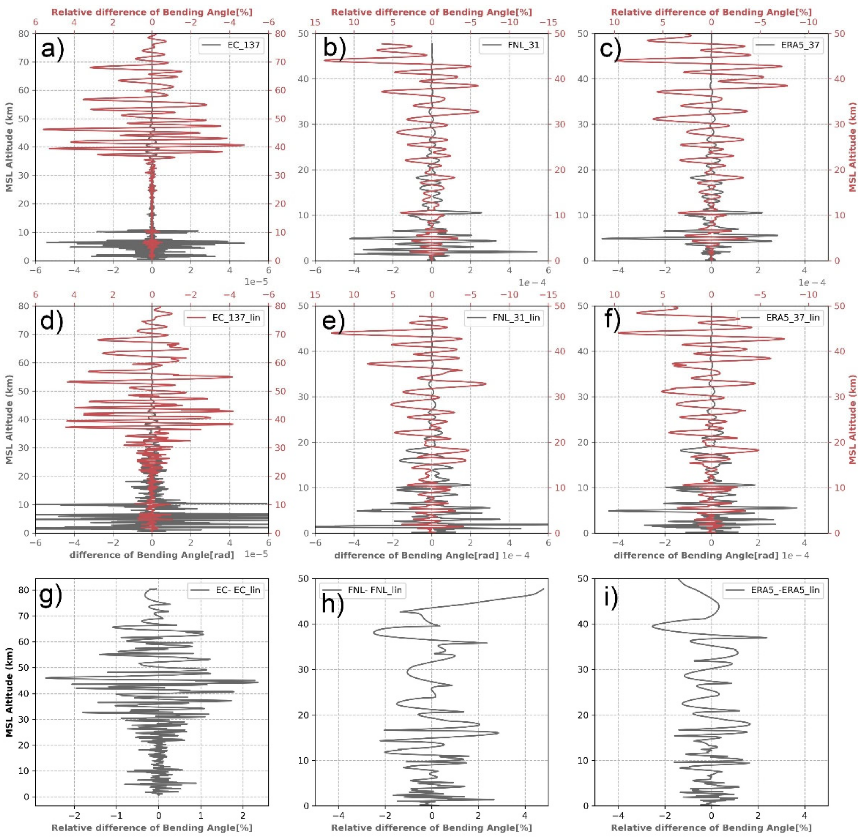
3.2. Experiment 2: Evaluation of the Error of the FM on the Fixed Model Level

Experiment 1 identified the exp algorithm with the log-cubic interpolation as the ideal FM owing to its high accuracy. Therefore, when computation efficiency is the primary focus, the exp algorithm with the log-linear interpolation is also considered. This experiment tested the extent of errors of the FMs. Another factor that introduced error to the FM is the model level (resolution of vertical levels). Thus, in this experiment, we chose three widely used analyses with different levels: 137 levels EC4Dvar, 31 levels FNL, and 37 levels of ERA5. The refractivity profiles of these analyses were all simulated by FY3D level 2 refractivity products. During this simulation, FY3D data were first interpolated into a resolution of 20 m and then extracted according to the model level. Subsequently, each simulated analysis was transformed to the BA via the FMs. Next, the results were compared with the FM true value, providing FY3D level 2 product refractivity profiles. Their RDs and differences are listed at the end, which can provide an error reference for the FM under the model levels considered here.

Figure 6 shows how the level interval, indicated by the rainbow colors, affects the RD ((E_BA − T_BA)/T_BA × 100%). In general, the less the interval, the less is the RD. EC4Dvar’s RD is less than the RDs for others because of the higher resolution of its levels. For example, EC4Dvar’s resolution is less than 1 km below 35 km, and its RD is less than ±0.5%. By contrast, the errors for FNL and ERA5 are less than ±1% for heights of 0–30 km owing to their low resolution. Interestingly, ERA5 and FNL show similar vertical resolution. However, the RD for ERA5 below 10 km is mostly less than that for FNL. This is because the Abel integral integrates values from lower levels to higher levels, and ERA5 owns the other six levels (i.e., 875, 825, 775, 225, 175, and 125 hPa), which ensures more accurate interpolation results for ERA5. Figure 6 also shows the comparison of the log-cubic interpolation (a–c) with log-linear interpolation (d–f). The errors of the latter are 1–2% larger than those of the former owing to the lower interpolation accuracy of log-linear.

Figure 7 compares the results of the RD (a–c) and difference (d–f) of the exp algorithm with log-cubic interpolation on the model levels of the three analyses.

Below 35 km, the RD and difference for EC4Dvar are less than ±0.5% and ±0.5 × 10⁻⁵, respectively, while those for FNL and ERA5 frequently oscillate in the range of ±2% to ±4%. Above 35 km, the RD and difference for EC4Dvar are similar to those for FNL and ERA5. The large bias for FNL and ERA5 resulted from two aspects: (i) the low resolution of the level interval; (ii) the rapid change in the atmospheric condition below 10 km. In such conditions, if the vertical grid density of refractivity profiles is insufficient, a larger oscillation of BA profiles will occur. The same comparison as Figure 7 but for log-linear interpolation is shown in Figure A6 in Appendix B.

Figure 8a–f concludes the detailed errors, the difference (grey), and RD (red) for forward-modeled three analyses, which are listed in

Table 2. RD and difference for forward modeled analyses in MLS (mean sea level, km).

Statistics	MSL Height (km)	Order of Magnitude	EC 4Dvar (cubic)	EC 4Dvar (lin)	Msl Height (km)	FNL(31) (cubic)	ERA5(37) (cubic)
Relative difference (RD)	0–35	%	$\pm$0.5%	$\pm$1%	0–30	$\pm$2.5%	3%
	35–58		$\pm$4%	$\pm$4%	30–40	$\pm$5%	5%
	58–80		$\pm$1.8%	$\pm$2%	40–50	$\pm$15%	10%
Difference	0–10	1 × 10−5	$\pm$4 × 10−5	$\pm$6 × 10−5	0–11	$\pm$4 × 10−4	$\pm$2 × 10−4
	10–35	1 × 10−6	$\pm$2 × 10−6	$\pm$8 × 10−6	11–22	$\pm$4 × 10−5	$\pm$5 × 10−5
	35–50	1 × 10−6	$\pm$3 × 10−6	$\pm$4 × 10−6	22–40	$\pm$2 × 10−5	$\pm$2 × 10−5
	50–60	1 × 10−7	$\pm$2 × 10−7	$\pm$4 × 10−7	40–46	$\pm$2 × 10−6	$\pm$2 × 10−6
	60–80	1 × 10−7	$\pm$4 × 10−8	$\pm$6 × 10−8	46–50	$\pm$6 × 10−6	$\pm$6 × 10−6

. Figure 8g–i concludes the difference in the RD between two interpolation methods based on each analysis. Below 30 km, the RD of log-cubic interpolation is 0.5–1% lower than that of log-linear interpolation, 2% lower for 30–50 km, and back to 1% lower for a height above 50 km. For FNL, the log-cubic results are 2% lower than the results of log-linear. For ERA5, the log-cubic results are 1.8% lower than the results of log-linear.

4. Discussion

An FM plays an important role during GNSS RO data processing and assimilation. The more accurate the FM, the more accurate are the two processes. Although the Abel algorithm and interpolation methods separately are sufficiently discussed, to the best of our knowledge, there has been no systematic discussion on the combination of interpolation and integration methods. In addition, no results on estimating the error of an FM on a fixed model level, for example 137 EC, have been reported.

In this study, we first reviewed the principles of four Abel integral methods. Subsequently, we conducted experiment 1 to compare three Abel integral algorithms (i.e., direct, exp, and exp_T) and two interpolation methods (i.e., log-cubic and log-linear) via the mean value analysis of the difference and relative difference between the experimental value (forward-modeled EC4Dvar) and true value (FY3D BA). The results suggested that (1) the exp algorithm with log-cubic interpolation is the most accurate one in every level because it has better integral accuracy (errors approximately 2%) to inputs, especially when the input is lower than an order of magnitude of 1 × 10⁻² (that is, above a height of 60 km). Above this height, the direct algorithm induced a 10% error. (2) When errors exist in inputs, the exp algorithm tends to amplify the error compared with the direct algorithm. (3) The exp algorithm with log-linear interpolation is often feasible for its computation efficiency. Its errors were 0.2%, −2%, and −20% larger than those of log-cubic for the heights of 5–50, 55–65, and 70–80 km, respectively. (4) The improvement of exp_T algorithm to the exp algorithm is limited. Our results are consistent with results of [35,36].

Subsequently, we conducted experiment 2 to determine the exact errors caused by the exp algorithm, which would be affected by the level interval of inputs. Therefore, we selected refractivity profiles on model levels of three widely used analyses (i.e., 137 levels of EC4Dvar, 31 FNL, and 37 ERA5) as the inputs. Results demonstrated that the forward-modeled BA of denser resolution analysis EC4Dvar was closer to the true value FY3D. The errors of the exp algorithm with log-cubic and log-linear were less than 1% and 0.5% below 38 km, less than 4% within 38–50 km, and less than 1.8% and 2% above 58 km, respectively. By contrast, the other two analyses had low accuracy. Our results are in good agreement with the results of [28].

This study paves a way to better understand the errors of the FM in RO data assimilation and processing. Simulation errors on model levels of three analyses can be a helpful FM error reference. This experiment only compared direct, exp, and exp_T algorithms, while excluding the fourth Abel integral: the linear algorithm. Such an algorithm is not feasible for data assimilation but can be used in RO data processing. In the future, linear algorithm and other integral algorithms can be addressed to compare the FM. Regarding the interpolation method, we only considered log-linear and log-cubic interpolation methods, which might have inferior representativeness above 60 km, where the interval is too large. Machine learning methods might be resorted to solve this problem.

References

1. Cardinali, C.; Healy, S. Impact of Gps Radio Occultation Measurements in the Ecmwf System Using Adjoint-Based Diagnostics. Q. J. R. Meteorol. Soc. 2014, 140, 2315–2320. [Google Scholar] [CrossRef]
2. Sun, Y.; Bai, W.; Liu, C.; Yan, L.; Du, Q.; Wang, X.; Yang, G.; Mi, L.; Yang, Z.; Zhang, X. The Fengyun-3c Radio Occultation Sounder Gnos: A Review of the Mission and Its Early Results and Science Applications. Atmos. Meas. Tech. 2018, 11, 5797–5811. [Google Scholar] [CrossRef] [Green Version]
3. Schreiner, W.S.; Weiss, J.P.; Anthes, R.A.; Braun, J.; Chu, V.; Fong, J.; Hunt, D.; Kuo, Y.; Meehan, T.; Serafino, W.; et al. Cosmic-2 Radio Occultation Constellation: First Results. Geophys. Res. Lett. 2020, 47. [Google Scholar] [CrossRef]
4. Bai, W.; Tan, G.; Sun, Y.; Xia, J.; Cheng, C.; Du, Q.; Wang, X.; Yang, G.; Liao, M.; Liu, Y.; et al. Comparison and Validation of the Ionospheric Climatological Morphology of Fy3c/Gnos with Cosmic During the Recent Low Solar Activity Period. Remote Sens. 2019, 11, 2686. [Google Scholar] [CrossRef] [Green Version]
5. Liao, M.; Healy, S.; Zhang, P. Processing and Quality Control of Fy-3c gnos Data Used in Numerical Weather Prediction Applications. Atmos. Meas. Tech. 2019, 12, 2679–2692. [Google Scholar] [CrossRef] [Green Version]
6. Oscar. Available online: https://www.wmo-sat.info/oscar/gapanalyses?mission=9 (accessed on 15 August 2021).
7. Bai, W.; Deng, N.; Sun, Y.; Du, Q.; Xia, J.; Wang, X.; Meng, X.; Zhao, D.; Liu, C.; Tan, G.; et al. Applications of Gnss-Ro to Numerical Weather Prediction and Tropical Cyclone Forecast. Atmosphere 2020, 11, 1204. [Google Scholar] [CrossRef]
8. Harnisch, F. Scaling of Gnss Radio Occultation Impact with Observation Number Using an Ensemble of Data Assimilations. Mon. Weather. Rev. 2013, 141, 4395–4413. [Google Scholar] [CrossRef]
9. ECMWF Observation Monitoring. Available online: https://www.ecmwf.int/en/forecasts/charts/obstat/gpsro_gpsro__count_0001_plot_o_count_gpsro_gpsro?facets=Parameter,Bending%20angles&time=2021062100&Phase=Setting (accessed on 22 June 2021).
10. Bowler, N.E. An Assessment of Gnss Radio Occultation Data Produced by Spire. Q. J. R. Meteorol. Soc. 2020, 146, 3772–3788. [Google Scholar] [CrossRef]
11. Bai, W.; Sun, Y.; Du, Q.; Yang, G.; Yang, Z.; Zhang, P.; Bi, Y.; Wang, X.; Wang, D.; Meng, X. An Introduction to FY3 GNOS in-Orbit Performance and Preliminary Validation Results. In Proceedings of the EGU General Assembly Conference, Vienna, Austria, 27 April–2 May 2014. [Google Scholar]
12. Bai, W. An Introduction to the Fy3 Gnos Instrument and Mountain-Top Tests. Atmos. Meas. Tech. 2014, 7, 1817–1823. [Google Scholar] [CrossRef] [Green Version]
13. Liao, M. Preliminary Validation of the Refractivity from the New Radio Occultation Sounder Gnos/Fy-3c. Atmos. Meas. Tech. 2016, 9, 781–792. [Google Scholar] [CrossRef] [Green Version]
14. Steiner, A.K.; Ladstädter, F.; Ao, C.O.; Gleisner, H.; Ho, S.; Hunt, D.; Schmidt, T.; Foelsche, U.; Kirchengast, G.; Kuo, Y.; et al. Consistency and Structural Uncertainty of Multi-Mission Gps Radio Occultation Records. Atmos. Meas. Tech. 2020, 13, 2547–2575. [Google Scholar] [CrossRef]
15. Bi, Y.; Yuan, B.; Wang, Y.; Ma, G.; Zhang, P. Assimilation experiment of GPS bending angle using WRF model — analysis of impact on Typhoon “SinLaku”. J. Tropical Meteorol. 2013, 29, 149–154. [Google Scholar]
16. Gorbunov, M.; Stefanescu, R.; Irisov, V.; Zupanski, D. Variational Assimilation of Radio Occultation Observations into Numerical Weather Prediction Models: Equations, Strategies, and Algorithms. Remote Sens. 2019, 11, 2886. [Google Scholar] [CrossRef] [Green Version]
17. Bai, W.; Tan, G.; Sun, Y.; Xia, J.; Du, Q.; Yang, G.; Meng, X.; Zhao, D.; Liu, C.; Cai, Y.; et al. Global Comparison of F2-Layer Peak Parameters Estimated by Iri-2016 with Ionospheric Radio Occultation Data During Solar Minimum. IEEE Access 2021, 9, 8920–8934. [Google Scholar] [CrossRef]
18. Liu, C.; Kirchengast, G.; Syndergaard, S.; Schwaerz, M.; Danzer, J.; Sun, Y. New higher-order correction of GNSS RO bending angles accounting for ionospheric asymmetry: Evaluation of performance and added value. Remote Sens. 2020, 12, 3637. [Google Scholar]
19. Gorbunov, M.E. Ionospheric Correction and Statistical Optimization of Radio Occultation Data. Radio Sci. 2002, 37, 1–9. [Google Scholar] [CrossRef] [Green Version]
20. Hedin, A.E. Extension of the Msis Thermosphere Model into the Middle and Lower Atmosphere. J. Geophys. Res. Space Phys. 1991, 96, 1159–1172. [Google Scholar] [CrossRef]
21. Scherllin-Pirscher, B.; Syndergaard, S.; Foelsche, U.; Lauritsen, K.B. Generation of a Bending Angle Radio Occultation Climatology (Baroclim) and Its Use in Radio Occultation Retrievals. Atmos. Meas. Tech. 2015, 8, 109–124. [Google Scholar] [CrossRef] [Green Version]
22. Hocke, K. Inversion of Gps Meteorology Data. In Paper presented at the Annales Geophysicae 1997. In Proceedings of the Annales Geophysicae, Vienna, Austria, 30 April 1997. [Google Scholar]
23. Healy, S.B.; Thépaut, J.N. Assimilation Experiments with Champ Gps Radio Occultation Measurements. Q. J. R. Meteorol. Soc. 2006, 132, 605–623. [Google Scholar] [CrossRef]
24. Burrows, C.; Healy, S.; Culverwell, I. Improvements to the Ropp Refractivity and Bending Angle Operators. 2013. Available online: https://www.romsaf.org/general-documents/rsr/rsr_15.pdf (accessed on 22 June 2021).
25. Kursinski, E.R.; Hajj, G.A.; Schofield, J.T.; Linfield, R.P.; Hardy, K.R. Observing Earth’s Atmosphere with Radio Occultation Measurements Using the Global Positioning System. J. Geophys. Res. Atmos. 1997, 102, 23429–23465. [Google Scholar] [CrossRef]
26. The ROM SAF Consortium, some. The Radio Occultation Processing Package (Ropp) Forward Model Module User Guide. 2019.
27. Cucurull, L.; Derber, J.C.; Purser, R.J. A Bending Angle Forward Operator for Global Positioning System Radio Occultation Measurements. J. Geophys. Res. Atmos. 2013, 118, 14–28. [Google Scholar] [CrossRef]
28. Gilpin, S.; Anthes, R.; Sokolovskiy, S. Sensitivity of Forward-Modeled Bending Angles to Vertical Interpolation of Refractivity for Radio Occultation Data Assimilation. Mon. Weather Rev. 2019, 147, 269–289. [Google Scholar] [CrossRef] [Green Version]
29. Brenot, H.; Rohm, W.; Kačmařík, M.; Möller, G.; Sá, A.; Tondaś, D.; Rapant, L.; Biondi, R.; Manning, T.; Champollion, C. Cross-Comparison and Methodological Improvement in Gps Tomography. Remote. Sens. 2019, 12, 30. [Google Scholar] [CrossRef] [Green Version]
30. Xu, X.; Zou, X. Comparison of Metop-A/-B GRAS Radio Occultation Data Processed by CDAAC and ROM. GPS Solut. 2020, 24, 1–16. [Google Scholar] [CrossRef]
31. Zou, X.; Zeng, Z. A Quality Control Procedure for Gps Radio Occultation Data. J. Geophys. Res. 2006, 111, 111. [Google Scholar] [CrossRef] [Green Version]
32. Lohmann, M.S. Analysis of Global Positioning System (Gps) Radio Occultation Measurement Errors Based on Satellite De Aplicaciones Cientificas-C (Sac-C) Gps Radio Occultation Data Recorded in Open-Loop and Phase-Locked-Loop Mode. J. Geophys. Res. 2007, 112, 112. [Google Scholar] [CrossRef] [Green Version]
33. Savitzky, A.; Golay, M.J.E. Smoothing and Differentiation of Data by Simplified Least Squares Procedures. Anal. Chem. 1964, 36, 1627–1639. [Google Scholar] [CrossRef]
34. Orszag, S.A. On the Elimination of Aliasing in Finite-Difference Schemes by Filtering High-Wavenumber Components. J. Atmos. Sci. 1971, 28, 1074. [Google Scholar] [CrossRef] [Green Version]
35. Lewis, H. Abel Integral Calculations in Ropp. 2008. Available online: https://www.romsaf.org/general-documents/gsr/gsr_04.pdf (accessed on 22 June 2021).
36. Burrows, C.P.; Healy, S.B.; Culverwell, I.D. Improving the Bias Characteristics of the Ropp Refractivity and Bending Angle Operators. Atmos. Meas. Tech. 2014, 7, 3445–3458. [Google Scholar] [CrossRef] [Green Version]
37. Fjeldbo, G.; Kliore, G.; Eshleman, V. The Neutral Atmosphere of Venus as Studied with the Mariner V Radio Occultation Experiments. Astron. J. 1970, 76, 123. [Google Scholar] [CrossRef]
38. Yan, H.; Fu, Y.; Hong, Z. Spaceborne Gps Meteorology and Retrieval Technique (Chinese Version); Science and technology of China Press: Beijing, China, 2007. [Google Scholar]
39. Jin, S.; Cardellach, E.; Xie, F. Gnss Remote Sensing; Springer: Berlin/Heidelberg, Germany, 2014; Volume 16. [Google Scholar]
40. Marquardt, C.; Healy, S.; Luntama, J.; McKernan, E. GRAS Level 1 B Product Validation with 1d-Var Retrieval. EUMETSAT: Darmstadt, Germany, 2004. [Google Scholar]
41. Hickstein, D.D.; Gibson, S.T.; Yurchak, R.; Das, D.D.; Ryazanov, M. A Direct Comparison of High-Speed Methods for the Numerical Abel Transform. Rev. Sci. Instrum. 2019, 90, 065115. [Google Scholar] [CrossRef]
42. Schweitzer, S.; Pirscher, B.; Pock, M.; Ladstädter, F.; Borsche, M.; Foelsche, U.; Fritzer, J.; Kirchengast, G. End-to-End Generic Occultation Performance Simulation and Processing System Egops: Enhancement of Gps Ro Data Processing and Ir Laser Occultation Capabilities. University of Graz, Graz, Austria: Wegener Center for Climate and Global Change (WegCenter). 2008. Available online: http://wegcwww.uni-graz.at/publ/wegcpubl/arsclisys/2008/igam7www_sschweitzeretal-wegctechrepfffg-alr-no1-2008.pdf (accessed on 22 June 2021).
43. Sheng, F.X. Atmospheric Physics; Peking University Press: Beijing, China, 2013. [Google Scholar]
44. Lewis, H. Error Function Calculation in Ropp. 2007. Available online: https://www.romsaf.org/general-documents/gsr/gsr_04.pdf (accessed on 22 June 2021).
45. Lanzante, J.R.R. Robust and Non-Parametric Techniques for the Analysis of Climate Data: Theory and Examples, Including Applications to Historical Radiosonde Station Data. Int. J. Climatol. A J. R. Meteorol. Soc. 1996, 16, 1197–1226. [Google Scholar] [CrossRef]
Figure 1. Flow chart for experiment 1, the algorithm comparison.
Remotesensing 14 01081 g001
Figure 2. Flow chart of experiment two, evaluation of forward modeled analysis.
Remotesensing 14 01081 g002
Figure 3. Difference between the BA of FY3D (T) and EC4Dvar BA (E) using the direct and exp Abel integral algorithms, together with log-linear and log-cubic interpolation methods. (a,b) (Eexp/dir − T) using the log-cubic interpolation; (c,d) difference of the Abel integral algorithms (Edir − Eexp) based on the log-linear and log-cubic interpolation, respectively; (e,f) difference of interpolation methods (Elin − E) based on exp and direct Abel integral algorithms, respectively.
Remotesensing 14 01081 g003
Figure 4. RD of the BAs of FY3D (T) and EC4Dvar (E) based on the direct and exp Abel integral algorithms, with log-linear and log-cubic interpolation methods. (ac) (E − T)/T, where E can be calculated by either the exp or direct algorithm, with both interpolation methods; (df) (E1 − E2)/E2, where 1, 2 indicate two different FMs.
Remotesensing 14 01081 g004
Figure 5. Difference (first row) and RD (second row) between the exp_T and exp algorithms.
Remotesensing 14 01081 g005
Figure 6. Effects of various model level intervals (km) on the FM error. The x-axis represents the RD, ((E − T)/T × 100%), of the BA between true value (T) and three simulated analyses (E): (a,d) 137 levels of EC4Dvar; (b,e) 31 levels of FNL; (c,f) 37 levels of ERA5. The FM is the exp algorithm, together with (ac) log-cubic or (df) log-linear.
Remotesensing 14 01081 g006
Figure 7. Under various model levels, the difference (ac) and RD (df) of FM based on the exp algorithm and log-cubic interpolation. The RD for EC4Dvar below 35 km is less than ± 0.5%, whereas RDs for FNL and ERA5 below 35 km are less than ± 5%. Above 35 km, the RD for EC4Dvar is less than ± 5%, while RDs for FNL and ERA5 are up to 10%.
Remotesensing 14 01081 g007
Figure 8. BA difference ( E T , in gray) and RD ( E T ) / T , in red) for EC4Dvar, FNL, ERA5, and FY3D based on the exp algorithm and log-cubic interpolation (ac) and log-linear interpolation (df). (gi) The difference between the RD of log-cubic interpolation and that of log-linear interpolation.
Remotesensing 14 01081 g008