Abstract
Air–sea fluxes are greatly enhanced by the winds and vertical exchanges generated by mesoscale convective systems (MCSs). In contrast to global numerical weather prediction models, space-borne scatterometers are able to resolve the small-scale wind variability in and near MCSs at the ocean surface. Downbursts of heavy rain in MCSs produce strong gusts and large divergence and vorticity in surface winds. In this paper, 12.5 km wind fields from the ASCAT-A and ASCAT-B tandem mission, collocated with short time series of Meteosat Second Generation 3 km rain fields, are used to quantify correlations between wind divergence and rain in the Inter-Tropical Convergence Zone (ITCZ) of the Atlantic Ocean. We show that when there is extreme rain, there is extreme convergence/divergence in the vicinity. Probability distributions for wind divergence and rain rates were found to be heavy-tailed: exponential tails for wind divergence (P∼ with slopes that flatten with increasing rain rate), and power-law tails for rain rates (P∼ with a slower and approximately equal decay for the extremes of convergence and divergence). Co-occurring points are tabulated in two-by-two contingency tables from which cross-correlations are calculated in terms of the odds and odds ratio for each time lag in the collocation. The odds ratio for extreme convergence and extreme divergence both have a well-defined peak. The divergence time lag is close to zero, while it is 30 min for the convergence peak, implying that extreme rain generally appears after (lags) extreme convergence. The temporal scale of moist convection is thus determined by the slower updraft process, as expected. A structural analysis was carried out that demonstrates consistency with the known structure of MCSs. This work demonstrates that (tandem) ASCAT winds are well suited for air–sea exchange studies in moist convection.
1. Introduction
The interaction of the atmosphere with the ocean is strongest in the tropics, where deep convection and rain-induced downbursts drive intense vertical exchanges of momentum, heat, and moisture. Under the right conditions, these moist convective processes organize upscale through aggregation of individual cloud systems (thunderstorms) into a mesoscale convective system (MCS)—a large contiguous area of convective and stratiform rain spanning about 100 km or more in at least one horizontal direction that can persist for several hours [1]. Examples of MCSs over the tropical ocean include tropical cyclones and squall lines, and they are found embedded in tropical waves, superclusters, and the Madden–Julian oscillation. MCSs and other forms of organized convection are absent from contemporary global numerical weather prediction (NWP) and global climate models (GCMs) due to insufficient numerical resolution and inadequate parameterizations [2,3]. Furthermore, the global observing system does not allow the 4D tracking of these small-scale processes in NWP data assimilation [4]. As a result, further theoretical and observational studies are necessary to support the appropriate representation of these processes in GCMs.
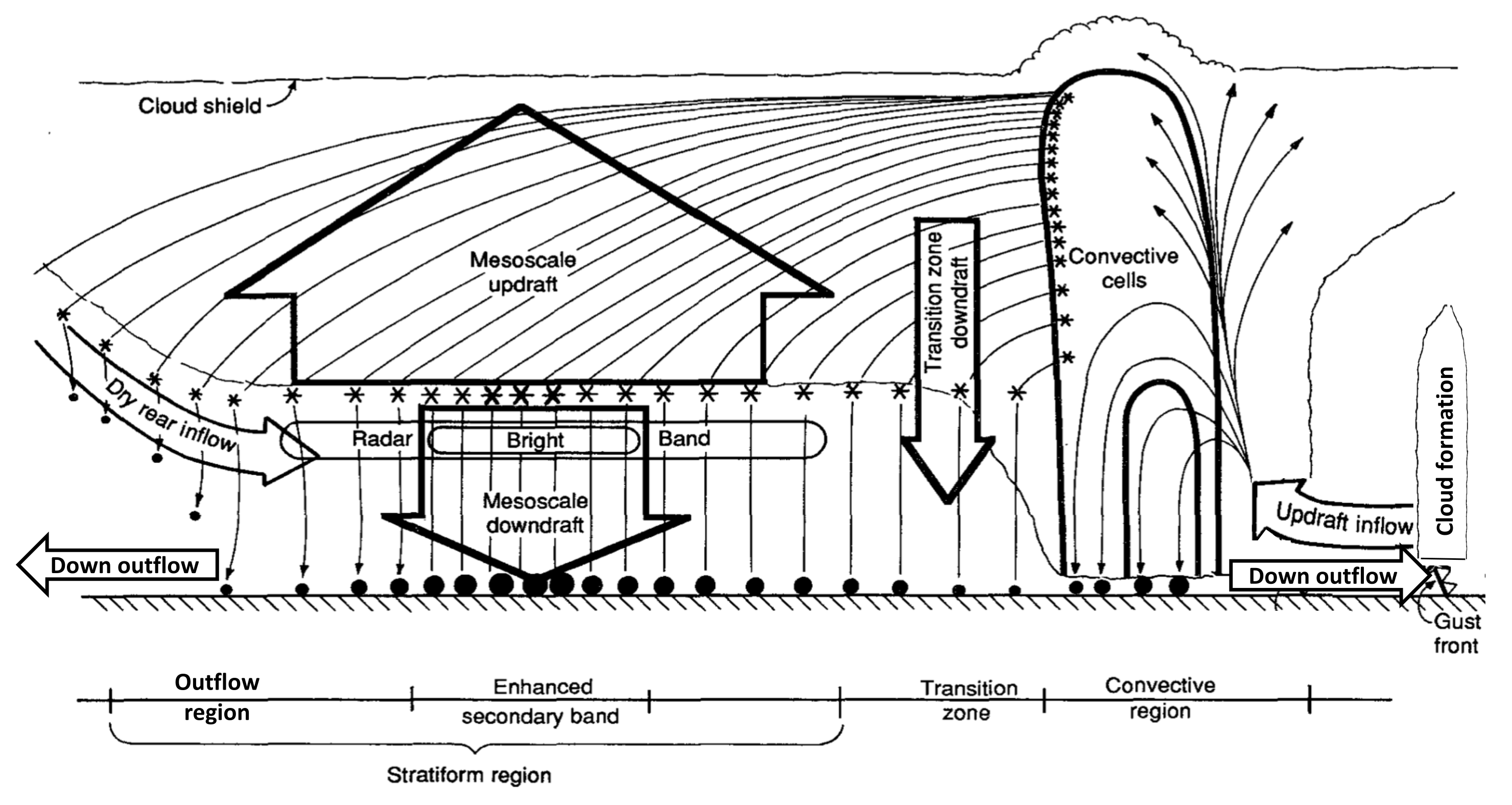
A conceptual model of a mature MCS and the relationship between its spatial structure and precipitation intensity are shown in Figure 1 (see Refs. [1,5]). Precipitating clouds are organized horizontally into three regions: a stratiform region, a convective region, and a narrow transition zone linking the two. The convective region consists of young, active deep convection where moist surface air is drawn in and carried upwards in strong (5–10 m s) convective-scale (∼10 km) updrafts to the top of the tropopause, where it diverges and spreads out. The moist updraft air rises, expands, cools, and then condenses into cloud and rain drops, which freeze when lifted above the 0 C level. Condensation and freezing releases heat into the air, increasing its buoyancy and uplift. As the convective updraft ages, vertical air motion weakens to the extent that aggregated precipitating particles fall out, melting and evaporating on the way down, cooling the surrounding air and forcing it to descend and diverge near the ocean surface in strong downdrafts. The collective outflow of cold air from the downdrafts of individual convective cells spreads out horizontally, displacing the warmer boundary layer air to form a cold pool at the surface, and a gust front at its periphery, which in turn promotes more deep convection. In the transition zone, convective cells age and decay such that vertical air motions weaken to the point that the level of peak convergence slopes upward until it sits atop the melting layer (appearing on radar as a “bright band”). Now the MCS has a stratiform structure consisting of two layers: an upper level dominated by weak updrafts (mesoscale updraft) and a lower level dominated by weak downdrafts (mesoscale downdraft). Hydrometeor trajectories are shown illustrating the process of fall speed sorting, differential hydrometeor source-region altitude, and nonuniform vertical air motions through the stratiform region. Clearly, the interaction of rain and wind is fundamental to the existence of MCSs.

Figure 1.
Conceptual model of a mesoscale convective system showing 2D hydrometeor trajectories through stratiform region of a squall line with trailing stratiform precipitation. (Modified from original ([5]) to show surface winds). Reprinted with permission from Ref. [5]. Copyright 1991 American Meteorological Society.
The small-scale wind variability in and near MCSs can be resolved by C-band fixed fan-beam space-borne scatterometers, such as the advanced scatterometer (ASCAT) on-board the MetOp series of satellites [6,7,8,9,10,11,12]. The potential of ASCAT to detect the horizontal wind divergence associated with individual MCS downdrafts was investigated by Kilpatrick and Xie [9], who concluded that ASCAT could reliably detect mesoscale (100–300 km) downdrafts, but not convective-scale (5–20 km) gust fronts. However, that conclusion was based on an analysis that did not include wind vectors from areas with rain rates greater than 3 mmh. The exclusion of such data was based on rain contamination problems experienced with Ku-band QuikSCAT winds. However, quality assessment studies showed that ASCAT winds are much less affected by rain than Ku-band scatterometer winds [13].
Rain contamination (i.e., signal attenuation, volume scattering from drops, and rain splashing and capillary wave attenuation effects at the surface) of the radar signal was shown to be small for ASCAT [6,7] (see also [14,15]), while the presence of rain, downdrafts, and updrafts increases the variability of the wind within a wind vector cell (WVC, the area from which radar backscatter is received and processed to produce a wind vector (c.f., [16])). This enhanced subcell wind variability increases the wind representativeness error in NWP model and buoy comparisons and leads to some uncertainty in the interpretation of ASCAT retrieved wind quality in triple collocation analyses [8]. Furthermore, it degrades even more NWP wind quality, since NWP models are unable to resolve the rain-induced dynamics [8]. Thus, the consistency between ASCAT, buoy, and NWP winds is not reduced by rain contamination, but mainly by the strong local wind gradients associated with heavy rain [7]. As a result, Lin et al. [8] concluded that in applications such as nowcasting and oceanography, flagged winds should be kept since they contain essential information on gustiness and air–sea interaction processes. That conclusion is supported by Priftis et al. [10], who combined ASCAT with Next Generation Weather Radar (NEXRAD), soundings, and buoys to explore wind structures produced by oceanic MCSs near two coastal locations in the United States. Using all ASCAT winds, regions of convergence and divergence within the MCSs, as well as outflow boundaries associated with downdrafts, were successfully identified.
The above studies demonstrate that ASCAT-derived wind fields and their spatial derivatives contain useful information on the interaction between winds and rain. A next step is to quantify that information in ways that can help improve parameterizations of moist convection. If simultaneous and reliable measurements of wind and rain fields were possible, then it would be straightforward to calculate and analyze space–time correlations. At present that is not possible. (However, such simultaneous measurements will be acquired in the future (from 2024 approximately), as the Metop Second Generation (Metop-SG) satellite series will carry on board the C-band scatterometer SCA and the high-frequency microwave radiometer MWI.) On the other hand, correlations can be investigated in a more limited way using ASCAT winds from the ASCAT triple configuration (i.e., ASCAT-A, B, and C on-board MetOp-A, B, and C, respectively, separated in time by 50 min (max)) collocated with rain fields retrieved from Meteosat Second Generation (MSG) geostationary imagery (namely, the daytime MSG rain product produced by the Royal Netherlands Meteorological Institute (KNMI)). One such collocation is illustrated in Figure 2. This figure shows wind vectors in the overlapped portion of two ASCAT swaths in the tandem configuration together with contours of a time-collocated MSG rain field. Note that the modification of the observed wind field (within 50 min) by the presence of heavy rain is remarkable and extends up to a few hundred kilometers from the rain cell location. Note also the areas of strongly converging and diverging wind vectors (pointed to in the figure by the letters C and D). These features occur near convective rain cells (>10 mm h), implying the presence of updrafts, downdrafts, and gust fronts associated to moist convection and precipitation. Finally, note that MSG geostationary rain products are available every 15 min and are therefore particularly suitable to study fast moist convection processes.
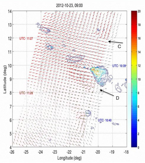
Figure 2.
A satellite view of interaction of rain and ocean winds in Atlantic Inter-Tropical Convergence Zone in an area a few degrees north of equator to west of coast of Africa. Figure shows superposition of wind vectors from ASCAT-A (black) and ASCAT-B (red) with contours of Meteosat Second Generation (MSG) rain at time corresponding to pass of ASCAT-A. Colorbar shows rain rate in mmh. Note convective rain cells (>10 mmh) and nearby areas of strong wind convergence (C) and divergence (D).
The purpose of this paper is to present a statistical approach to identify and quantify correlations between MSG rain rates and ASCAT wind divergence. We focus our attention on MSCs in the Atlantic Intertropical Convergence Zone where MCSs are plentiful, rainfall is intense, and deep convection extends from the surface to the tropopause, strongly coupling the surface with the upper troposphere. Preliminary to the correlation analysis is the need to regrid MSG rain rates to the swath grid. One approach is to regrid with the WVC average rain rate (cf. [17]). However, for our purposes, that choice is undesirable as averaging can mask the presence of convective-scale downbursts—even a single downburst in a WVC has the potential to produce significant wind gusts. Therefore, we elected to regrid with the WVC maximum rain rate.
As will be shown, the scattergram of wind divergence vs rain rate shows a strongly nonlinear correlation, and the probability distributions of each variable are found to be heavy-tailed with a non-extreme core (a Gaussian core in the case of wind divergence). This invites thinking in terms of extreme values and a data classification that highlights the extremes of convergence, divergence, and rain. The key result is that the extremes of rain are shown to correlate with the extremes of wind divergence.
An early version of the work presented here was reported in [18]. Since then, we learned that a methodology similar to ours is used to correlate weather extremes with climate extremes. For example, Martius et al. [19] and Zscheischler et al. [20] correlated wind speed extremes with precipitation extremes. Key differences between their work and ours are (i) the motivation (assessing climate risks vs improving parameterizations of organized convection), and (ii) the data and scales of interest (ERA-40 100 km gridded daily data vs high resolution wind (12.5 km) and rain (3 km) acquired in minutes by satellite instruments). [Note that ERA essentially misses the substantial variability induced by fast moist convection processes [3].]
The paper is organized as follows. The data and study area are described in Section 2. Section 3 describes the methods used to calculate and classify wind divergence and regrid and classify rain rates, while Section 4 describes the methods used to correlate the two fields. The results of the correlation analysis are given in Section 5, and a brief summary and ideas for future work are given in Section 6.
2. Data and Study Area
2.1. ASCAT Winds
Currently there are three ASCAT scatterometers in orbit: ASCAT-A on MetOp-A (launched in October 2006 and decommissioned November 2021), ASCAT-B on MetOp-B (September 2012), and ASCAT-C on MetOp-C (November 2018). The data used in this paper were collected before the launch of MetOp-C. The MetOp satellites are operated by the European Organisation for the Exploitation of Meteorological Satellites (EUMETSAT). They are in quasi-sun-synchronous orbits with an inclination angle of , and cross the equator at about 09:30 (descending pass) and 21:30 (ascending pass). The ASCAT scatterometer uses a dual-swath fan-beam configuration with two 550 km wide swaths separated by a nadir gap of about 700 km. The fan-beam configuration has consistent measurement geometry and instrument performance. ASCAT transmits at C-band frequencies (5.3 GHz) [21], which results in winds that are much less affected by rain clouds than winds derived by the higher Ku-band frequency scatterometers, i.e., the higher Ku-band radar frequency results in about a 40-fold higher impact of rain attenuation and scattering [13,14].
In the configuration before MetOp-C, MetOp-A and MetOp-B flew in tandem with overlapping swaths in the tropics (see Figure 3), such that the left (right) swath of ASCAT-A overlaps the right (left) swath of ASCAT-B, with a 50 min difference. Their orbits are such that the order they cross the equator alternates: half the time the crossing order is AB, and other half BA. Therefore, in this paper we relabel the scatterometers to reflect their crossing order: the earlier scatterometer is labeled SCAT-1 and crosses the study area at time ; the later scatterometer is labeled SCAT-2 and crosses at time . In this paper, only data from SCAT-1 are analyzed; an analysis of the changes that occur between the SCAT-1 and SCAT-2 passes (e.g., see Figure 2) is left for a future study.

Figure 3.
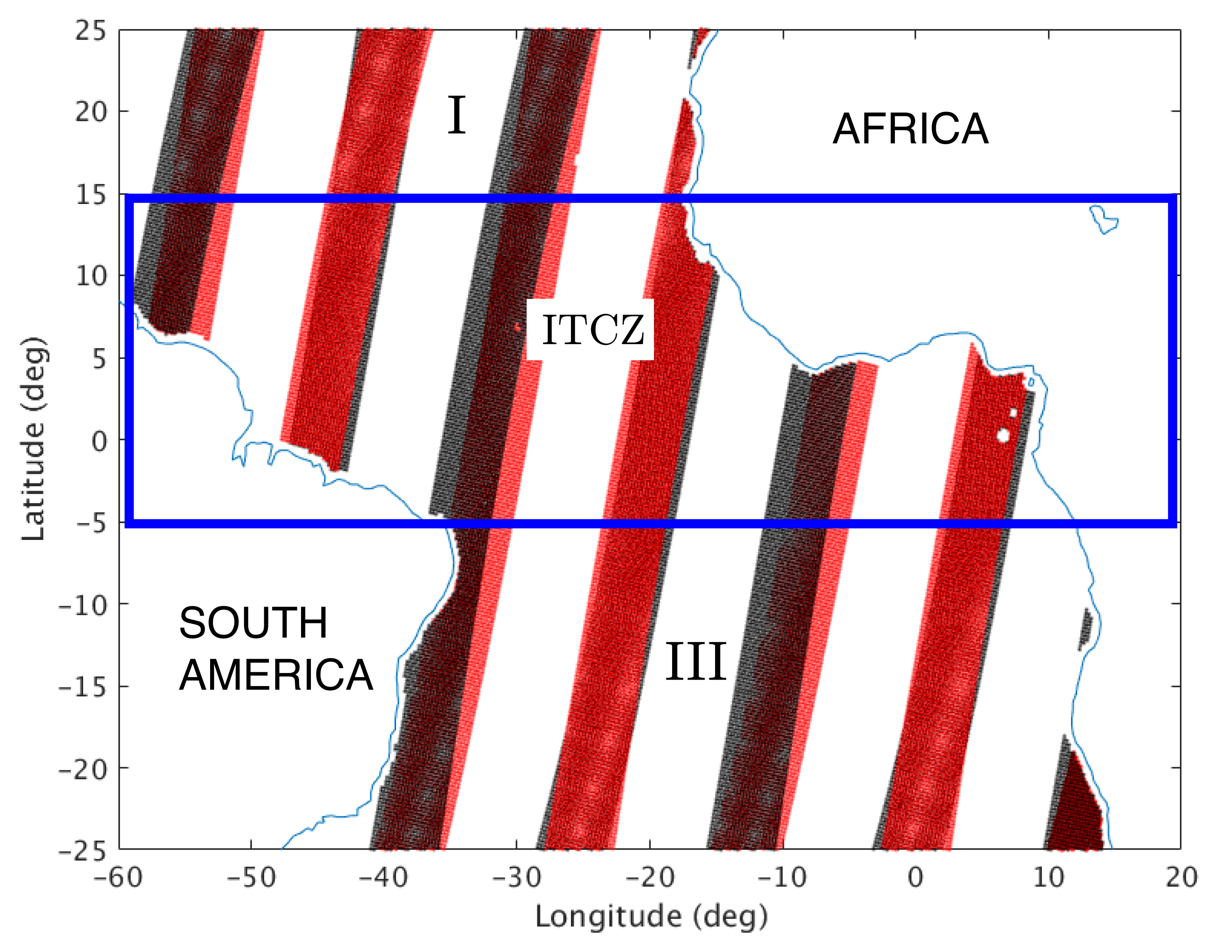
Overlapped portions of ASCAT-A (red) and -B (black) swaths over Tropical Atlantic. Tropics are divided into three latitude bands. Main region of interest lies within rectangle, labeled ITCZ. Latitude band to its north is labeled Region I, and to its south, Region III. In the tropics, half of the time the right swath of ASCAT-A overlaps the left swath of ASCAT-B and vice versa. The left edge of the later scatterometer is shifted slightly eastward relative to the earlier scatterometer. To distinguish the time-of-arrival, the scatterometers are re-labeled SCAT-1 and SCAT-2. In the figure, the SCAT-2 swath overlies the SCAT-1 swath.
The radar backscatter detected by ASCAT is processed and presented on a 12.5 km grid expressed in a coordinate system attached to the moving satellite (the swath grid). The axes parallel and perpendicular to satellite motion are called, respectively, the along-track and cross-track directions. Grid points are located at the center of wind vector cells (WVCs)—the area from which radar backscatter is received and processed to produce a wind vector (c.f., [16]).
The radar backscatter goes through two levels of processing. Level-1 processing involves averaging individual backscatter measurements and produces them on a regularly spaced grid. Level-2 takes the Level-1 data and applies inversion and ambiguity removal. The empirically derived geophysical model function (GMF), which relates the radar backscatter to the 10-meter-height stress equivalent wind speed and direction [22], is inverted. Due to the highly nonlinear nature of the GMF and the presence of measurement errors, the inversion procedure usually yields multiple solutions, referred to as ambiguities. An ambiguity removal algorithm is applied to produce ’selected’ winds. Several quality control (QC) steps are carried out, before and after inversion [6], as well as during ambiguity removal. The Level-2 processing is carried out at the Royal Netherlands Meteorological Institute (KNMI) using the EUMETSAT Numerical Weather Prediction Satellite Application Facility (NWP-SAF) ASCAT Wind Data Processor (AWDP). The GMF used here in the AWDP is CMOD5, as explored in [23], and it is also the predecessor of CMOD7 [24]. Ambiguity removal is carried out using a 2D variational method (2DVAR) [25]. The wind inversion residual (MLE), used for QC, is a measure of WVC wind variability. As a result, unrepresentative winds in MCSs are flagged in the ASCAT products to avoid their use in NWP data assimilation where ocean moist convective processes are generally not well resolved. Note that the operational QC leads to about 0.3% of flagged ASCAT wind rejections in the region of interest (i.e., Tropical Atlantic). However, Lin et al. [8] concluded that rain-flagged winds, often associated with rain, should be kept in oceanography applications since they contain essential information on gustiness and air–sea interaction processes. Therefore, to fully analyze MCSs, all flagged winds are kept.
2.2. MSG Rain
Meteosat Second Generation (MSG) is a generation of geostationary satellites operated by EUMETSAT [26,27]. Continuous observation of the Earth’s full disk is achieved with the Spinning Enhanced Visible and Infrared Imager (SEVIRI) imaging radiometer. SEVIRI is a 12-channel imager, with 11 channels observing the Earth’s full disk with a 15-min repeat cycle at a nadir resolution of 3 km. SEVIRI measurements allow monitoring of the physical processes of clouds to determine their growth and microstructures. Rain rates are derived using the Cloud Physical Properties-Precipitation Properties (CPP-PP) algorithm [28,29]. Unlike radar data, the algorithm does not calibrate rain rates with surface rain-gauge measurements. Instead, and more relevant here, the algorithm estimates the rain rate per pixel from the cloud condensed water path, particle effective radius, cloud thermodynamic phase, and cloud top temperature retrieved from SEVIRI. Retrievals are limited to daytime hours (07:30–16:30 UTC) and solar zenith angles smaller than . The MSG rain product is available for the Atlantic Ocean, Europe, and Africa between longitudes and latitudes and has an accuracy of 1 mm h. Further information can be found on the KNMI web site at http://msgcpp.knmi.nl/ (accessed on 22 February 2022) [30].
2.3. Study Area
Figure 3 shows the Tropical Atlantic divided into three latitude bands. The focus of this paper is on the data from the region highlighted by the rectangle, which identifies the latitudes (S–N) between which the Inter-Tropical Convergence Zone (ITCZ) makes an annual migration (c.f., Waliser and Gautier [31]). The regions to the north and south of the ITCZ are: Region I, N–N; and Region III, S–S.
2.4. Collocations
A collocation data set was created consisting of six months of ASCAT winds and MSG rain: 425 in (Northern Hemisphere, NH) winter (December 2012–February 2013) and 376 in (NH) summer (June–August 2013). The MSG rain product is limited to daytime hours and this constrains the ASCAT winds to be from descending orbits only, with coverage between 08:30 UTC (eastern edge of the study area) and 13:30 UTC (western edge). All ASCAT swaths are at 9:30 local solar time (LST), implying that the left swath is at 9:08 LST and the right swath at 9:52 LST.
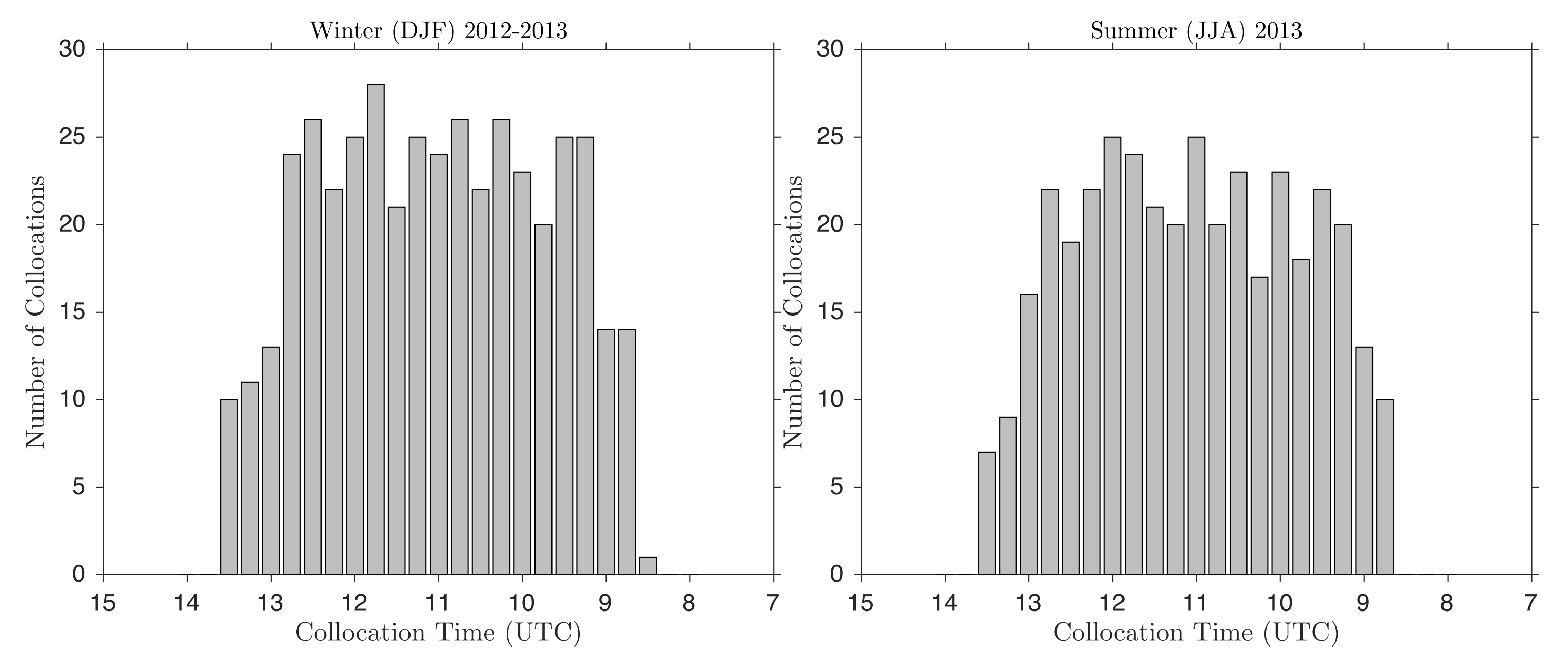
Each collocation consists of winds from the overlapped swaths of ASCAT-A and ASCAT-B (between latitudes S and N), and a sequence of 17 MSG rain fields beginning 2 h before the first scatterometer pass until 2 h after the pass of the second scatterometer. The rain fields stored in each collocation were limited in spatial extent to encompass the area spanned by the overlapped ASCAT-A and -B swaths. The number of collocations at different times of the day are shown in Figure 4. The histograms indicate no significant differences between winter and summer.
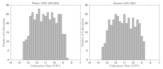
Figure 4.
Number of collocations in boreal winter (left) and boreal summer (right) versus collocation time (time recorded for middle MSG frame in each collocation). Collocations in most eastern part of study area occur at 08:30 UTC, while those in most western part occur at 13:30 UTC (see Figure 3). Total number of collocations is 801 (425 in winter and 376 in summer).
3. Wind Divergence and Regridded Rain
3.1. Wind Divergence Calculation
Wind speed and wind direction were converted to cross-track (x) and along-track (y) velocity components (see Appendix A). Wind gradients were estimated using central differences and were averaged locally to reduce noise. Since rain is a spatially highly variable quantity, the central difference-and-average (CDA) operations were carried out using the smallest possible area on the scatterometer grid—a two-by-two block of WVCs. For the block shown in Figure 5, wind divergence is estimated by:
where
and km is the grid spacing.
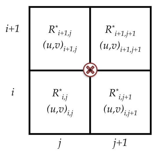
Figure 5.
Schematic for calculation of horizontal divergence and assignment of WVC rain rate. Wind divergence is assigned to half-grid point . is maximum MSG rain rate in area spanned by WVC .
The CDA two-by-two scheme was compared with standard central differences (CD), and a CDA three-by-three scheme (which averages over a larger area). Although the CDA two-by-two produces the noisiest estimate, a comparison of the probability distributions of showed that the three schemes produced equivalent statistics; in particular, all have heavy tails (see Appendix B). This gives confidence that the extreme values of reflect the information content in the scatterometer signal and are not a product of a noisy algorithm.
3.2. PDFs and Classification
3.2.1. PDF Characteristics
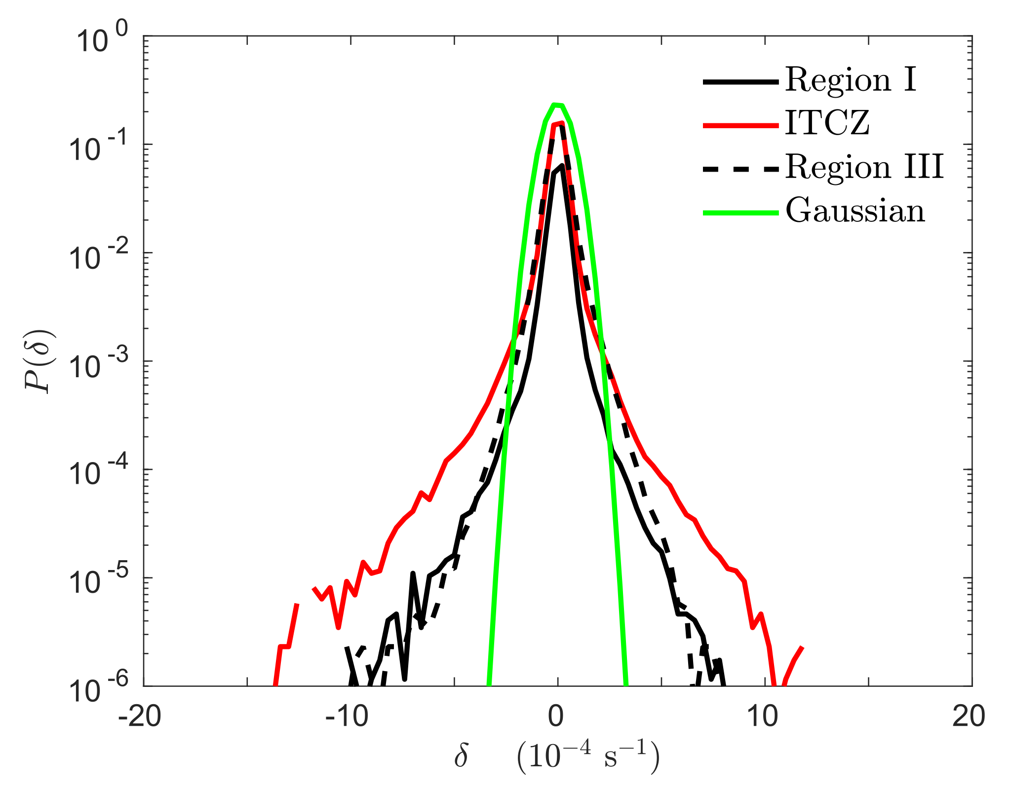
Wind divergence PDFs () for the three regions are compared in Figure 6. The observed PDFs are approximately symmetric about a central value. This suggests decomposing these PDFs into a Gaussian core with heavy tails to left and right. The ITCZ PDF has the heaviest tails as the ITCZ is the main area of MCS activity.
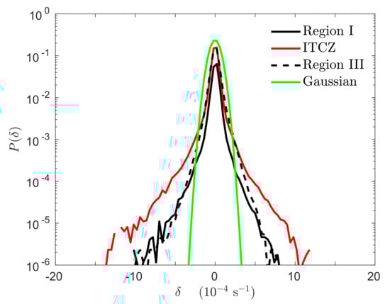
Figure 6.
PDFs of wind divergence for Regions I, ITCZ, and III (December 2012). Green curve is a Gaussian distribution with zero mean and standard deviation for all data ().
The first four statistical moments are compared in Table 1. All regions have a small mean wind divergence (). The ITCZ has the most storm activity, and in consequence has the largest variance, skewness and kurtosis.

Table 1.
Moments of for three regions (Figure 6) and for all data.
Skewness measures how far and in what direction a PDF deviates from left–right symmetry. Due to the strong convergence in the ITCZ, its skewness is large-negative (−0.77). The skewness is also negative in Region I (−0.18), but positive (greater divergence than convergence) in Region III (0.15), implying that it is a region characterized by subsidence. For all data, the skewness is large-negative (−0.32). This may be linked to the observed skewness of the tropospheric vertical motion PDF, probably due to latent heating, as seen in radiosonde ascent climatologies [32].
Kurtosis measures the heaviness of the tails, and therefore it indicates the magnitude and probability of extreme events. Table 1 shows that the ITCZ has a kurtosis eight times larger, and Regions I and III two times larger, than the kurtosis of a Gaussian. Indeed, the vigorous local dynamics involved with moist convection processes clearly add variability in the tails of the distribution.
3.2.2. Thresholds and Classification
A graphical technique, known as a ‘normal probability plot’, is used to define thresholds separating the tails from the Gaussian core. The technique is illustrated in Figure 7 for the ITCZ PDF; note that the figure does not show the full extent of the tails—only those values of between s (compare with Figure 6). Points falling on the slanted line are in the Gaussian core. Starting at about the 5th and 95th percentiles, the tails rapidly peel away from that line. The vertical lines in the figure () intersect the tails at the 2nd and 98th percentiles. Thus, can be construed as sharp thresholds defining the beginning of the left and right tails. Events in the left tail are convergence extremes and assigned the label ; events in the right tail are divergence extremes and assigned the label ; and events in the Gaussian core constitute the ‘background’ and are assigned the label . (For convenience, the preceding information is summarized in Table 2.) More thresholds could be introduced to further define a ‘transition’ region between the Gaussian core and the extremes, say, between the 2nd and 5th percentiles on the left and between the 95th and 98th percentiles on the right. However, this was not performed here.
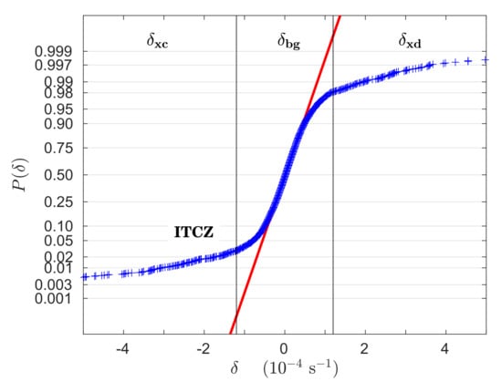
Figure 7.
Normal probability plot of ITCZ PDF. PDF follows a Gaussian distribution where it falls on or close to red line. Vertical lines () partition into extremes ( and ) and background (). Note that figure does not show full range of values. Left and right tails extend much further out (to about s)—see Figure 6.
Table 2.
Wind divergence classes and thresholds. Thresholds, , map to classes , where is standard deviation of all between 25S and 25N.
3.2.3. Are the Heavy Tails Geophysical?
Scatterometer signals are affected by rain and it is important to ask: do the heavy tails represent a real geophysical effect, or is the accuracy of the divergence calculation somehow compromised in rain conditions to produce artificially large δ? Assuming random retrieval errors in the wind components , the expected random error in may be estimated as . For km and extreme s, this implies a random wind error ms, which is a very extreme ASCAT error indeed [33] and unknown to the authors. Another possibility is that systematic errors might exist that produce large . However, this would imply some systematic negative neighbor correlation in wind component errors to enhance . Such error patterns are not found. Therefore, we conclude that the extreme values are reasonable, and hence the heavy tails are mostly geophysical, i.e., caused by the presence of strong wind gradients in strong convective scale updrafts and downdrafts in MCSs (cf. Figure 2).
3.3. Rain Classification and Regridding
3.3.1. Classification
MCSs are comprised of systems of precipitating clouds (e.g., [34]): (i) young, vigorous convection; (ii) stratiform cloud; and (iii) aging/decaying convection. The rain types associated to these cloud systems are convective rain (produced in young, vigorous convection and falls at rates in excess of 10 mm h[35,36,37]), and stratiform rain (produced in stratiform cloud and falls at rates between 1 and 10 mm h). Rain produced in aging/decaying convection is a mixture of convective and stratiform rain and falls at rates between about 5 and 10 mm h[38]. Based on this information, we define the following classes and thresholds: (1) Extreme rain (E): >10 mm h, (2) Transition rain (T), 5–10 mm h, (3) Stratiform rain (S): 1–5 mm h, (4) Light rain (L): 0–1 mm h, and (5) No Rain (): 0 mm h.
3.3.2. Regridding
Quantitative analysis requires regridding MSG rain to the wind and -grids. As noted earlier, averaging can mask the presence of extreme values. Therefore, rain was represented on the wind and grids using the WVC maximum rain rate. This choice allowed rain rates to be classified using the thresholds in Table 3. The regridding was carried out as follows: first, MSG 3 km rain cells are mapped to ASCAT WVCs. Second, wind grid point is assigned the WVC maximum rain rate . Then, because is calculated using a block of wind vectors, rain rates on the -grid are assigned the block maximum rain rate, denoted by , where:
Table 3.
Rain classes () and thresholds.
Both and are classified and labeled according to Table 3.
3.3.3. PDFs
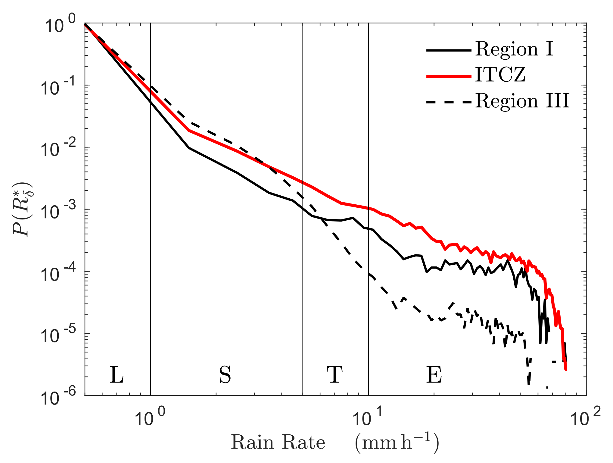
Figure 8 compares regional probability distributions, . The PDFs are compiled from the MSG collocated field nearest in time to the SCAT-1 pass. The log-log scale makes clear that follows a power-law, P∼, over the range 1–40 mm h. The power-law exponent is the same for Regions I and ITCZ, but due to the low level of convective activity, Region III has a steeper decay for rain rates greater than 5 mm h.
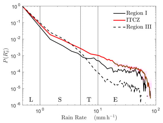
Figure 8.
Probability distribution of rain, , for Regions I, ITCZ, and III (December 2012). Rain classes are shown along bottom of plot.
4. Correlation Methods
4.1. Contingency Tables
Contingency tables follow a standard layout (Table 4). Let X and Y be two categorical variables, X with I categories and Y with J categories. The number of joint events is denoted by . Summing over an index is denoted by subscript +. Thus, is the number of observations, is the number of observations, and is the total number of observations ().
Table 4.
contingency table. Number of joint () events is denoted by . Subscript + denotes sum over index it replaces: is number of observations, is number of observations, and is total number of observations ().
The probability structure of Table 4 can be expressed in terms of joint probabilities, , and marginal probabilities and :
or in terms of conditional probabilities and :
4.2. Odds and Odd Ratios
Correlations are expressed in terms of the odds and odds ratio after regrouping and recoding variables X and Y to produce a table in terms of binary variables A and B (Table 5).
Table 5.
contingency table for binary variables A and B.
Odds are an expression of relative probabilities: if p is the probability that an event occurs and the probability that it does not occur, then the odds that the event does occur is . In the case of two binary variables A and B, is calculated from the conditional probabilities , and from . For example, for events :
and similarly for events :
The odds ratio characterizes the strength of the association between two binary variables A and B, comparing them symmetrically:
The odds ratio has the following properties:
- (i)
- Range: ;
- (ii)
- is symmetric: ;
- (iii)
- if , A and B are independent;
- (iv)
- if , then A and B are positively correlated (the presence of B raises the odds of A); and
- (v)
- if , A and B are negatively correlated (the presence of B reduces the odds of A).
5. Results and Discussion
5.1. Local Analysis
5.1.1. Spatial Distribution
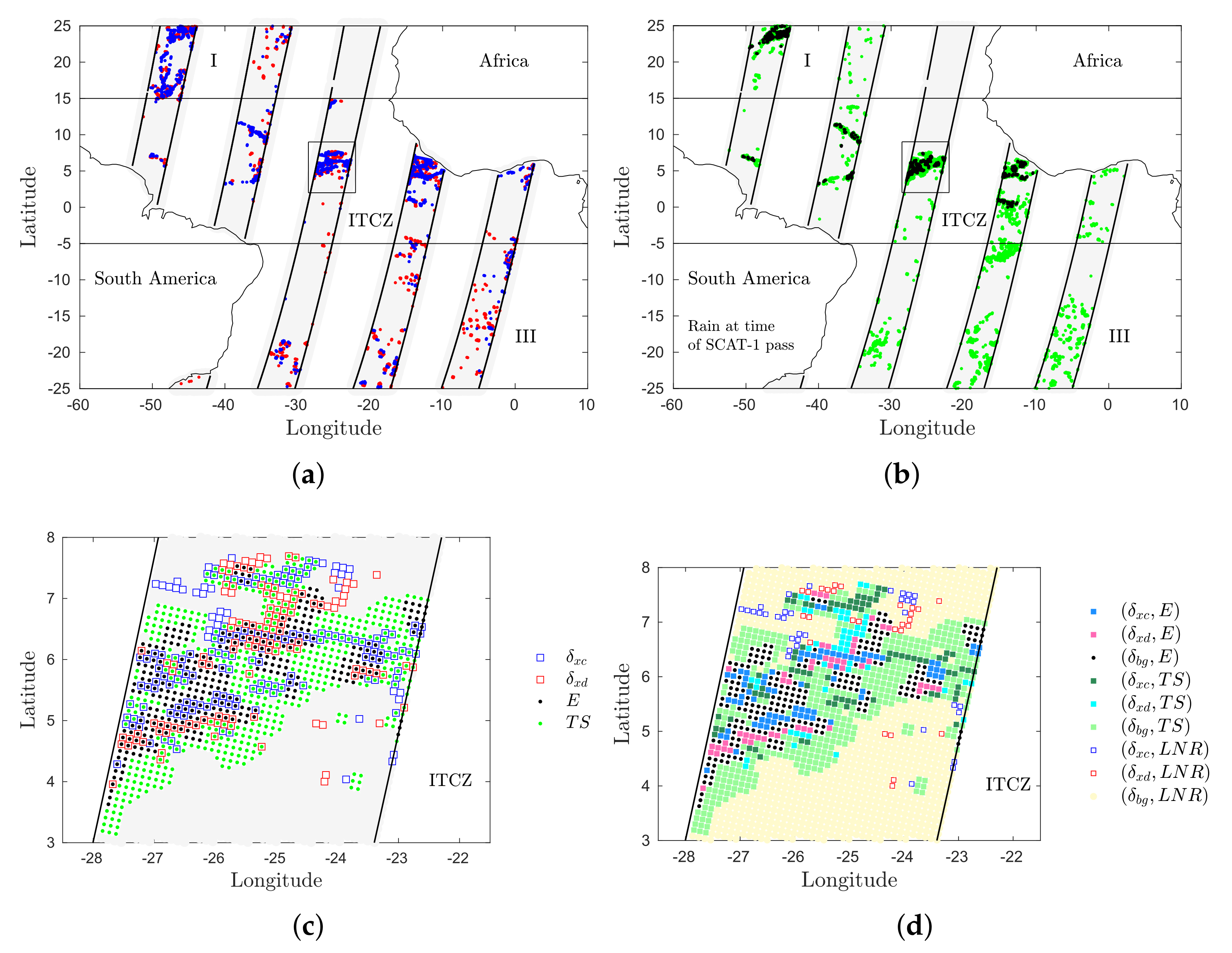
The spatial distribution of extremes and rain extremes is shown in Figure 9 for five successive SCAT-1 passes (ordered in time from left to right) on 5 December 2012: (in blue) and (in red) in Figure 9a; rain extremes (E in black) and transition/stratiform rain ( in green) in Figure 9b. The area outlined by the rectangles are combined in Figure 9c,d, with the former showing an overplot of the extremes and the latter a segmentation into subsets of co-occurring points defined by the two sets of thresholds. Subsets and are associated with moist convection dynamics, while subset is associated with common 3D turbulence processes.
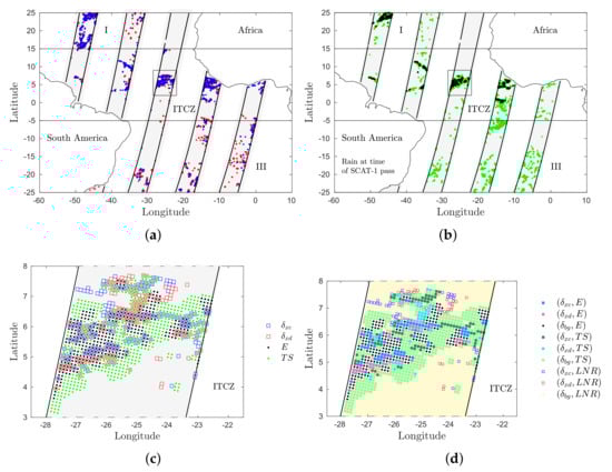
Figure 9.
Spatial patterns of extremes. (a) Extremes of convergence (blue) and divergence (red); (b) rain extremes (black) and transition/stratiform rain (green). Rain extremes are from field of view of ASCAT at time of the satellite pass. Times of five swaths are, from left-to-right, 09:45, 10:30, 11:15, 12:00, and 13:00 UTC. (c,d) Magnification of swath within the small rectangle in (a,b): (c) coinciding extremes. (d) Segmentation into subsets of co-occurring points defined by thresholds in Table 2 and Table 3.
Figure 9d shows that points in subset are close to convergence/divergence extremes, and hence candidates for reclassification (see below). There are also a few points in subsets and . These may be linked to dry convection, early [15] or late [24] stages of moist convection, and/or small convection cells (<3 km).
We now turn to a statistical analysis to determine the generality of the above observations and to estimate the form and strength of the correlation between and rain extremes.
5.1.2. Scatter Plot and Conditional Probabilities
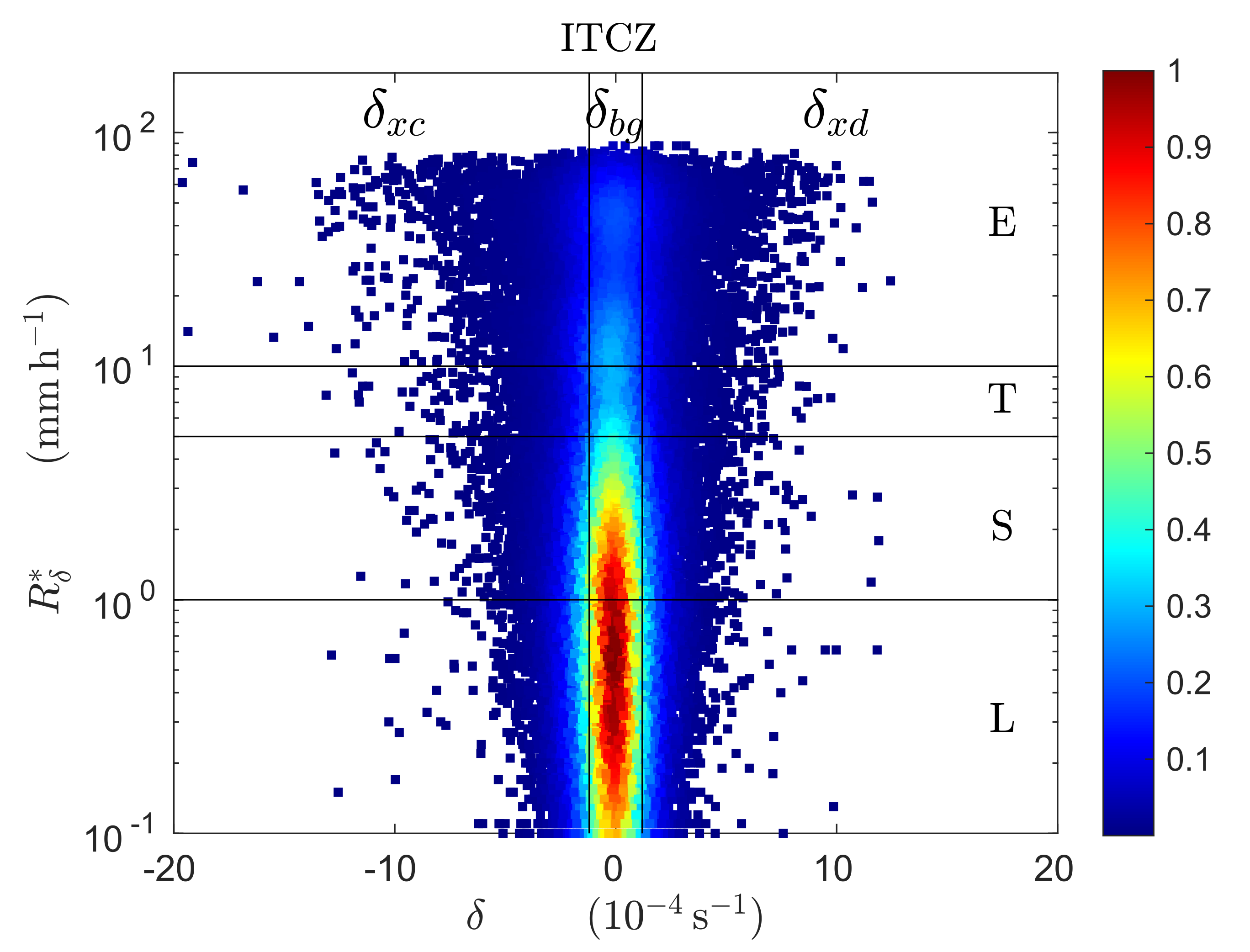
The statistical analysis uses all collocations during a one month period (here, December 2012). The data are pooled and plotted in a scattergram of vs. , which due to the large number of points is plotted here as a scatter density plot (Figure 10). Clearly the scatter is far from random and far from linear, but otherwise the functional form of the relationship is unclear. Progress is made by applying the class thresholds (the horizontal and vertical lines) to subset the data into slices.

Figure 10.
Scatter density plot of co-occurrences for the ITCZ.
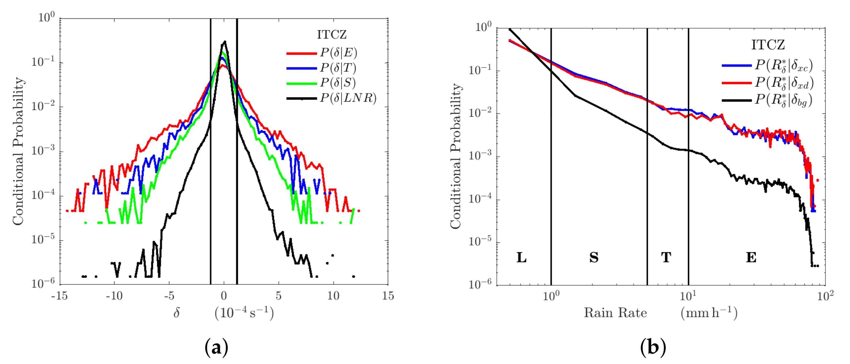
The data in each horizontal and vertical slice are summarized in a conditional PDF (Figure 11). The conditional PDF for horizontal slice i (rain class ) is denoted by . These are plotted semi-log in Figure 11a, which shows that the heavy tails are well described by an exponential decay, . The decay slowest for extreme rain and fastest for light or no rain.

Figure 11.
Probability structure of and for ITCZ: (a) conditioned on rain classes , and (b) conditioned on divergence classes .
Similarly, the conditional PDF for vertical slice j (divergence class ) is denoted by . These, however, are plotted log–log (Figure 11b), which shows that the heavy tails are well described by a power-law decay, , where . The decay is slower for the extremes ( and ) than for the background.
While a further analysis that estimates decay coefficients for rain and wind divergence would be useful in characterizing the tails of the distributions, this is beyond the scope of this paper, which is focused on assessing the connection between extreme rain and extreme divergence/convergence.
5.1.3. Contingency Tables
The intersecting thresholds partition the scattergram into a five-by-three array of boxes. The number in each box is entered into a five-by-three contingency table (Table 6a). This table is a discrete form of the scatter plot (Figure 10)—in physical terms, a simplified statistical representation of an MCS.
Table 6.
Two-way contingency table between categories of wind divergence () and rain intensity () and conditional probability structure for observations in December 2012.
Box contains all points classified as , and is the number of those points. Row normalization (i.e., by the number in horizontal slice i) yields discrete conditional probabilities (Table 6b). Thus, 20% of the points labeled E are also labeled (co-occur with) . Similarly, column normalization (i.e., by the number in vertical slice j) yields discrete conditional probabilities (Table 6c). Thus, 24% of the points labeled are also labeled E.
5.1.4. Correlating Extremes: The Two-By-Two Contingency Table and the Odds Ratio
The correlation of coextremes is calculated from the counts or probabilities in a two-by-two contingency table. The two-by-two table is created by merging cells in the five-by-three table. The new variables (A and B) are binary variables with a value indicating presence (1) or absence (0) at a grid point. For the case considered above, Table 7a is the result for , and Table 7b for .
Table 7.
Two-by-two contingency tables for coextremes of (a) rain and convergence (, ), and (b) rain and divergence (, ).
As described in Section 4.2, correlations are calculated using Equations (10)–(15). For the results in Table 7a,b, we obtain:
In both cases , implying a significantly positive correlation.
5.2. Structural Analysis
5.2.1. Spatial Structure and Reclassification
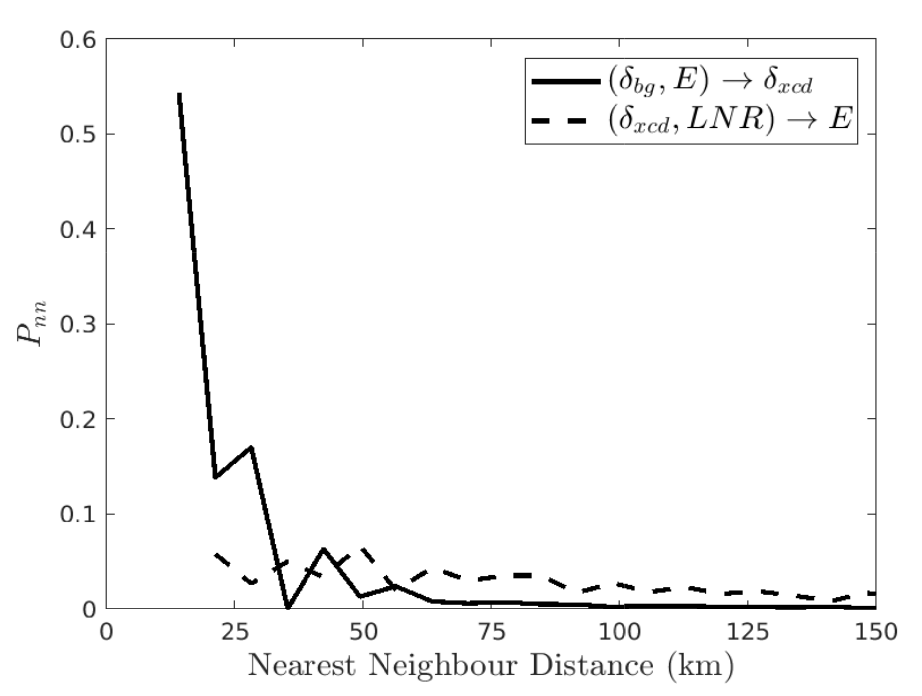
Table 6b shows that most rain extremes (viz, 64%) are in subset and Figure 9d shows that many of these are near convergence/divergence extremes. Therefore, it is reasonable to reclassify some of these if they are ’near enough’. To establish a distance criterion, we used all December 2012 data to calculate the nearest neighbor distribution, , where d is the distance from a point to its nearest convergence/divergence extreme. Figure 12 shows that (solid line) drops rapidly towards zero. About 70% of the were found to lie within 25 km of either a convergence or divergence extreme. Setting the distance threshold to 25 km, those points in the set that are within 25 km of a () are reclassified to (); ties are reassigned randomly to one of the two possibilities. The result is that reclassification modifies Table 7a,b so that increases by about 50% and decreases accordingly. This changes the numbers in Equation (16) to:

Figure 12.
Nearest neighbor distribution (using all observations in December 2012). Solid line: distance from points to the nearest . Dashed line: distance from points to nearest rain extreme E. Here , and .
–a three-fold increase in the odds ratio.
Table 6c also shows that about half of the extremes coincide with light or no rain, i.e., the subset . For this case, d is the distance from a point in to its nearest rain extreme E. Figure 12 shows that (dashed line) is small for all d. Only about 5% of the are within 25 km of a rain extreme, thus reclassifying them contributes only a small increase to (and corresponding decrease to ), and hence only a small increase in . We did not further test the occurrence of category E rain rates in preceding or following rain images, but we investigate rain and time lags below.
5.2.2. Temporal Evolution
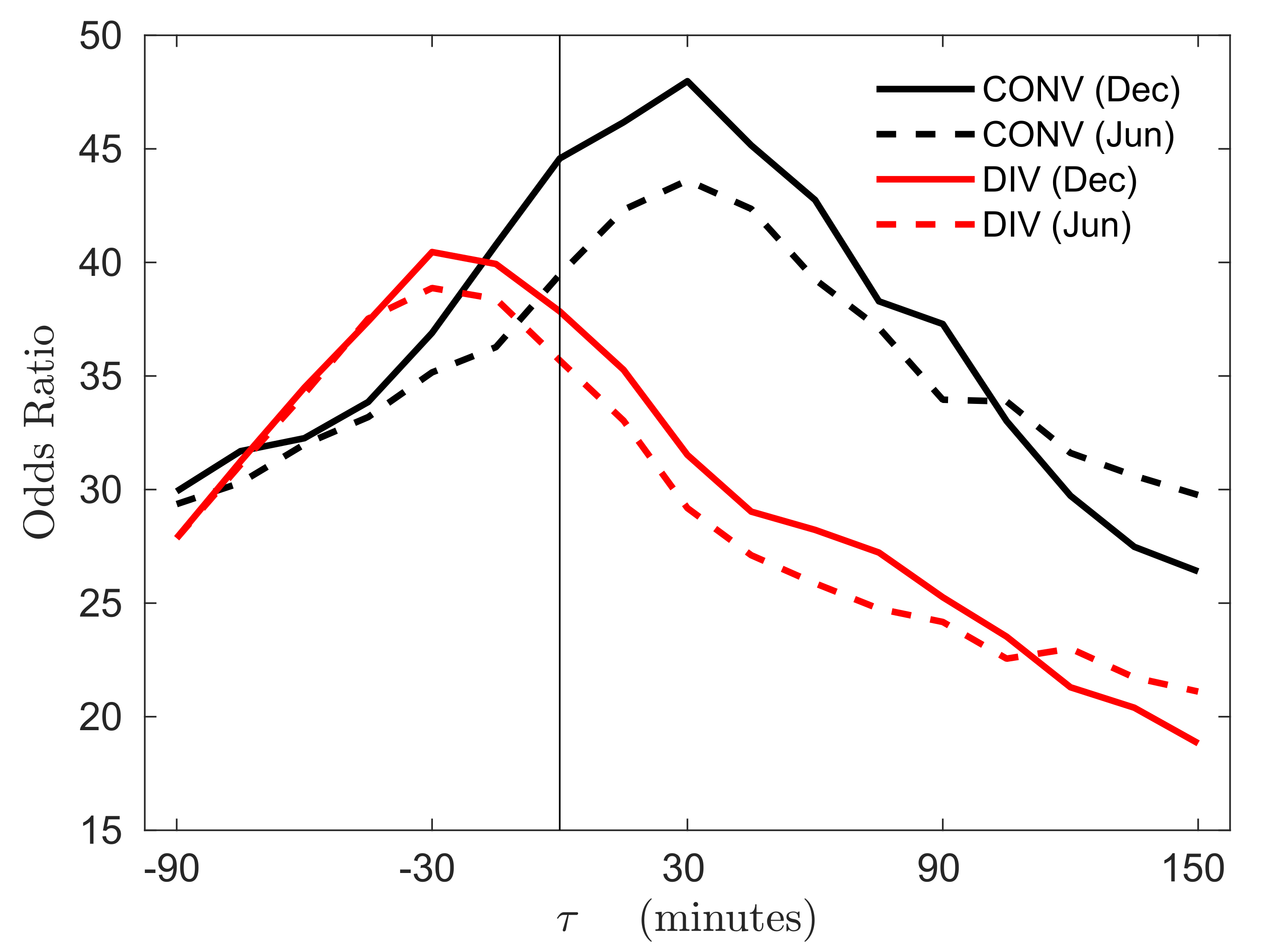
In Section 5.1.4 we calculated the odds ratio for rain product time lag (the time nearest to the SCAT-1 pass). Here, we investigate how the odds ratio evolves in time by tracking the local correlations. Results for a winter month (December 2012) and a summer month (June 2013) are shown in Figure 13. The effects of the reclassification described above are included, which increases the odds ratio by a factor of about 3.2 at each time lag. The figure shows that reaches a maximum at min (15 min before the SCAT-1 pass), implying that there is more extreme rain 15 min before the occurrence of extreme divergence, as depicted by SCAT-1 measurements, than at any other time. This is explained by the fact that rain falls fast: the most vigorous heat exchange between precipitation and air occurs at the melting and liquid stage, accelerating the cooled air downwards during the precipitation. At 20 ms, it takes rain drops about 4 min to fall over a 5 km height. For convergence (case (i)), reaches a maximum at min, implying that there is more extreme rain 30 min after the occurrence of extreme convergence, as depicted by SCAT-1 measurements, than at any other time. In other words, extreme rain generally appears some time after extreme convergence and closely precedes extreme divergence.
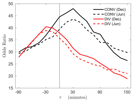
Figure 13.
Odds ratios for convergence (black) and divergence (red) for a winter month and a summer month. Rain product lag is relative to SCAT-1 pass ().
The overall conclusion is that the temporal scale of moist convection is determined by the slower updraft process, which is expressed in . Finally, varies in amplitude—larger in winter than in summer. In addition to the summer/winter differences, we also found intraseasonal and month-to-month variability (not shown), which is likely due to fluctuations in the ITCZ. A study of those fluctuations requires a data set spanning several years and is beyond the scope of this paper.
6. Summary and Future Work
In this paper we introduce and apply a novel approach to quantify the correlation between wind convergence/divergence with rain in the Atlantic Inter-Tropical Convergence Zone (ITCZ) using ASCAT 12.5 km winds collocated with a short time series of Meteosat Second Generation 3 km rain fields. Our approach was motivated by the observed statistics; namely, that the probability distributions for each variable were heavy-tailed and that it was the extremes of each variable that were associated with moist convection processes. A summary of our results now follows.
The variability of ASCAT scatterometer winds near rain was verified and shown to be associated with the passage of MCSs (Figure 2). Wind divergence was calculated from the observed winds. Inspection of wind divergence PDFs and calculation of its moments showed that it was negatively skewed and had heavy tails (Figure 6). Physically, heavy tails are due to the processes associated with the generation of convective rain: accelerated updrafts (due to condensation and freezing of water particles) leading to reinforced convergence, and nearby cool and dry downdrafts (due to precipitation, melting and evaporation) leading to reinforced divergence. With the aid of a normal probability plot (Figure 7), thresholds were defined to partition into three classes: background , convergence extremes , and divergence extremes .
To avoid loss of information about convective-scale rain events, MSG rain was represented by the local maximum rain rate: the WVC maximum rain rate () on the wind grid, and the two-by-two block maximum rain rate () on the grid. Rain classes were defined based on results of observational studies of rain produced in MCS precipitating clouds (): no rain , light rain , stratiform rain , transition rain , and extreme rain . Thresholds for these classes were based on results from many observational studies (Table 3). PDFs of the rain rates ‘seen’ by ASCAT were presented in Figure 8.
The correlation analysis proceeded in steps, starting with the scatter density plot (Figure 10), which showed that the correlation between and is neither random nor simple. Using the class thresholds, two ways to correlate the data were identified. One was to use the rain and thresholds to partition the data into horizontal and vertical slices and calculate conditional distributions. In the case of horizontal slices, the conditional distributions for each class (Figure 11a) show that the heavy left and right tails are approximately exponential: , with slopes that flatten with increasing rain intensity. In the case of vertical slices, conditional distributions for each class (Figure 11b) show that the heavy tails are described by a power-law: , with a slower and approximately equal decay for the extremes of convergence and divergence.
Correlations were also quantified by the odds ratio between and extremes (i.e., and ). Many extreme rain events were found to co-occur with background divergence. A structural analysis was carried out showing that many of these points were close to extreme convergence or divergence. Reclassifying those points increased the odds ratios by a factor of three, therefore greatly strengthening the correlation.
We also found many points of extreme convergence/divergence in areas of light or no rain. These may be related to dry convection, early [15] or late [24] stages of moist convection, and/or small convection cells (<3 km) rather than MCSs.
An important takeaway from the structural analysis is that the nearest neighbor distributions are consistent with the moist convective processes summarized in Figure 1, and hence reflect the known structure of MCSs. Further structural analysis of the data (e.g., using the radial distribution function) is possible and could be of interest.
Finally, the odds ratio was calculated as a function of time lag , which showed broad but well-defined peaks at a time lag of min for divergence and a lag of min for convergence (Figure 13), meaning that extreme rain lags extreme convergence by about 30 min, while extremes of rain closely precede divergence. This is consistent with descriptions of moist convection processes as described in the Introduction and conceptualized in Figure 1. This consistency and coherence in the winds and divergence patterns, as well as its credible association with independent rain products, may be further exploited to obtain improved statistical descriptions of tropical MCS dynamics and implied fluxes.
Future Work
Here we list some ideas for future work using the ASCAT-MSG collocations. First, recall that the 2D velocity gradient tensor, , can be decomposed as:
where , and are, respectively, the divergence, rate-of-strain and rate-of-rotation tensors. Thus, the analysis carried out in this paper should be extended to investigate and correlate strain rate extremes and vorticity extremes. Exploiting this additional information should improve the fluid dynamical picture of the rain-induced dynamics near MCSs.
Second, there may be multiple deep convection cells in a WVC, or a squall line of deep convection passing through a WVC. Obviously, the spatial organization of the convection affects convergence, divergence, and shear patterns. This organization should be investigated, which could be made more efficient using databases consisting of divergence/vorticity/strain features, and of MSG cloud and precipitation features, as was performed by [39] for observations from the Tropical Rainfall Measuring Mission (TRMM). Furthermore, applying additional statistical physics techniques to exploit the heterogeneous distribution of rain types in a WVC (e.g., using the radial distribution function), could reveal more structural information useful to modelers.
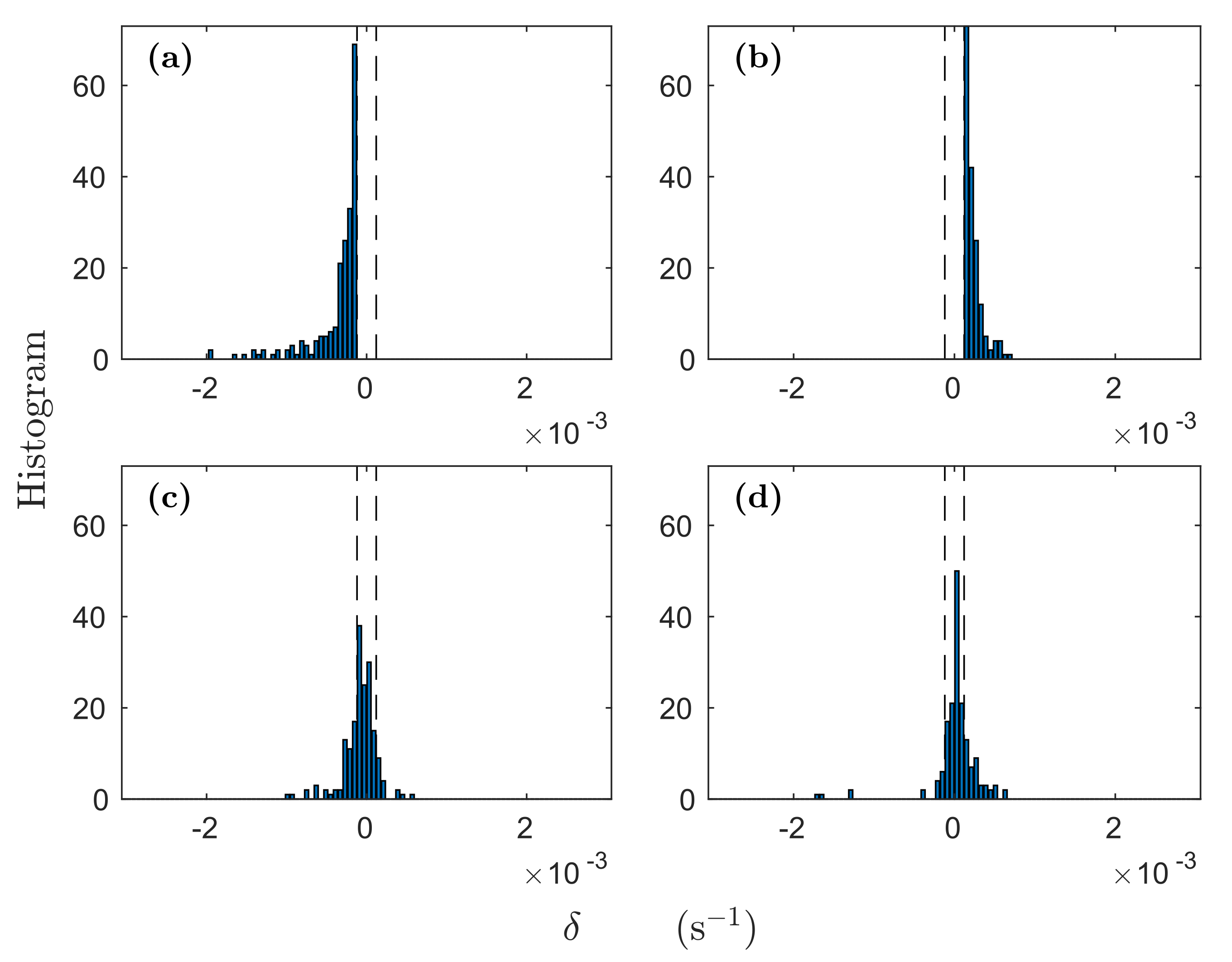
Third, there is information yet to be extracted about the time-dependent changes in the wind and rain fields from the overlapped SCAT-1 and SCAT-2 swaths. The scope of the present work did not permit us to do more than scratch the surface. A partial result that merely suggests a starting point for further work is shown in Figure 14. The results in the figures were extracted after identifying clusters of contiguous grid points with extreme values of the convergence/divergence in the SCAT-1 swath. The top panels in the figure show the result of pooling the statistics of all clusters (a) and clusters (b) seen by SCAT-1. The locations of these clusters were identified in the SCAT-2 fields and the statistics were again pooled (bottom panels). The change going from the top to the bottom panel demonstrates the rapid change that occurs in the wind field by rain-induced dynamics after only 50 min.
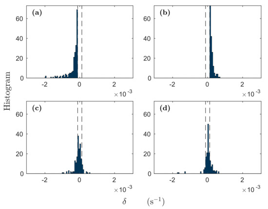
Figure 14.
Sample result that compares information in SCAT-1 with that in SCAT-2 (50 min later). The top panels (a,b) show, respectively, statistical distributions of extreme wind convergence () and divergence (), and bottom panels (c,d) show, for the same ocean areas, the change in SCAT-1 distributions after 50 min (SCAT-2 pass).
The availability of more than 14 years of high-resolution, accurate ASCAT-derived wind fields (and about nine years of tandem ASCAT A/B and/or B/C observations) should definitely be exploited to better characterize rain-induced dynamics. Of further relevance, the same analysis should be carried out with pencil-beam Ku-band scatterometers. The latter are known to be more sensitive to rain (which was recently better depicted in [40]). On the other hand, since they are rather noisy, spatial filters are applied, leading to rather smooth sea surface wind fields, as compared to that of fixed fan-beam C-band scatterometers (such as ASCAT). This will indeed impact their ability to capture extreme divergence/curl. However, a comprehensive analysis of the joint Ku-band and C-band scatterometer wind derivatives can help in improving the Ku-band wind derivatives near rain.
Finally, it is recommended that work be carried out in collaboration with modelers who can suggest further refinements in the analysis that can lead to improved parameterizations of moist convection.
Author Contributions
Author contributions to this paper were as follows: conceptualization, G.P.K., M.P. and A.S.; data curation, W.L.; formal analysis, G.P.K.; funding acquisition, M.P.; investigation, G.P.K.; methodology, G.P.K., M.P. and W.L.; project administration, M.P.; software, G.P.K.; writing—original draft, G.P.K.; writing—review & editing, M.P., W.L. and A.S. All authors have read and agreed to the published version of the manuscript.
Funding
This work was supported in part by the European Organization for the Exploitation of Meteorological Satellites Ocean and Sea Ice Satellite Application Facility (OSI-SAF) Visiting Scientist Program under reference OSI-SAF-AVS-15-02 and in part by the Spanish R&D projects L-BAND (ESP2017-89463-C3-1-R), which is funded by MCIN/AEI/10.13039/501100011033 and “ERDF A way of making Europe”, and INTERACT (PID2020-114623RB-C31), which is funded by MCIN/AEI/10.13039/501100011033. We also acknowledge funding from the Spanish government through the ‘Severo Ochoa Centre of Excellence’ accreditation (CEX2019-000928-S). The publication fee was partially supported by the CSIC Open Access Publication Support Initiative through its Unit of Information Resources for Research (URICI).
Data Availability Statement
Data supporting reported results can be found at: Meteosat Second Generation rain rates https://msgcpp.knmi.nl/ (accessed on 15 January 2022); wind divergence (as an L3 swath gridded (interpolated) product) at https://doi.org/10.48670/moi-00182 (accessed on 15 January 2022) (EU Copernicus Marine Service). The L3 product is produced by KNMI from L2 swath divergence and curl, which is available from KNMI on request (scat@knmi.nl).
Acknowledgments
This work is a contribution to CSIC PTI Teledetect. The ASCAT Level 2 data were provided by EUMETSAT and are accessible from https://osi-saf.eumetsat.int/ (accessed on 15 January 2022). The MSG precipitation data were provided by KNMI and can be accessed from https://msgcpp.knmi.nl/ (accessed on 15 January 2022). The software used in this paper was developed by the Royal Netherlands Meteorological Institute (KNMI) through the EUMETSAT Numerical Weather Prediction SAF (NWP-SAF). The authors thank Jan–Fokke Meirink (KNMI) for his help with the Meteosat Second Generation precipitation data used in this paper.
Conflicts of Interest
The authors declare no conflict of interest.
Appendix A. Wind Components
ASCAT wind vectors are supplied (in ASCAT BUFR files) as the 10-m stress equivalent wind speed [22] and wind direction (where is the direction in the meteorological convention, i.e., a zero degree direction means that the wind is blowing from the north). These are transformed to wind components in the cross-swath and along-swath directions by first transforming to zonal and meridional components :
and then to cross-swath and along-swath components :
where , are unit vectors related to the unit vectors and in the, respectively, zonal and meridional directions by:
The angle is the angle that makes with , which is given by:
where and depends on latitude. The method used to estimate is described in Vogelzang and Verhoef [41]. For the work in this paper, the code to calculate was extracted from the ‘convert’ library in the ASCAT Wind Data Processor (AWDP).
Appendix B. Comparison of Central Difference Schemes
Here, we compare the statistics of wind divergence () produced by the CDA two-by-two scheme with standard central differences (CD) and a CDA 3-by-3 scheme. The CDA two-by-two scheme is illustrated in Figure 5: x-derivatives are estimated by taking differences across columns and averaging along rows:
and y-derivatives are estimated by taking differences along rows and averaging across columns:
A statistical comparison of the three schemes is provided in Table A1 (first four moments) and Figure A1 (observed probability distributions).
The CDA two-by-two scheme is expected be noisier than the three-by-three scheme, and this is borne out by the table and figure: CDA two-by-two has the largest standard deviation, largest (negative) skewness, and largest kurtosis, while the three-by-three scheme has the smallest.
If after transforming to standardized coordinates the PDFs fall on the same curve, then they are statistically equivalent. Standardized coordinates (Z) are dimensionless and defined for variable x by:
where is the mean and the standard deviation. Of course, moments () of a standardized distribution are also dimensionless. They are calculated from:
where angle brackets denote an ensemble average. By construction the mean and variance are and . The third-order moment is the skewness (a measure of the PDF asymmetry) and the fourth-order moment is the kurtosis (a measure of the fatness of the PDF tails).
Figure A1 shows the PDFs in standardized coordinates for the three schemes. The three PDFs are nearly identical in the middle portion of their range, negatively skewed, and have fat but similar tails (large kurtosis). By eye, the differences between the tails of the PDFs appear small, leading to the expected conclusion that, neglecting the effects of noise and averaging, the PDFs are statistically equivalent. From Table A1, however, the variability in the kurtosis is large. That large variability in the kurtosis is at variance with the small variability in the PDFs serves as a reminder that one must exercise due caution when interpreting the kurtosis (and higher-order moments) of a noisy dataset potentially containing extreme events.

Figure A1.
Effect of numerical method on probability distributions calculated using standard central differences (CD 3-by-3, black), and difference-then-average (CDA 3-by-3, blue; CDA 2-by-2, red). Probability distributions are plotted in standardized coordinates, , where and are mean and standard deviation of , respectively.
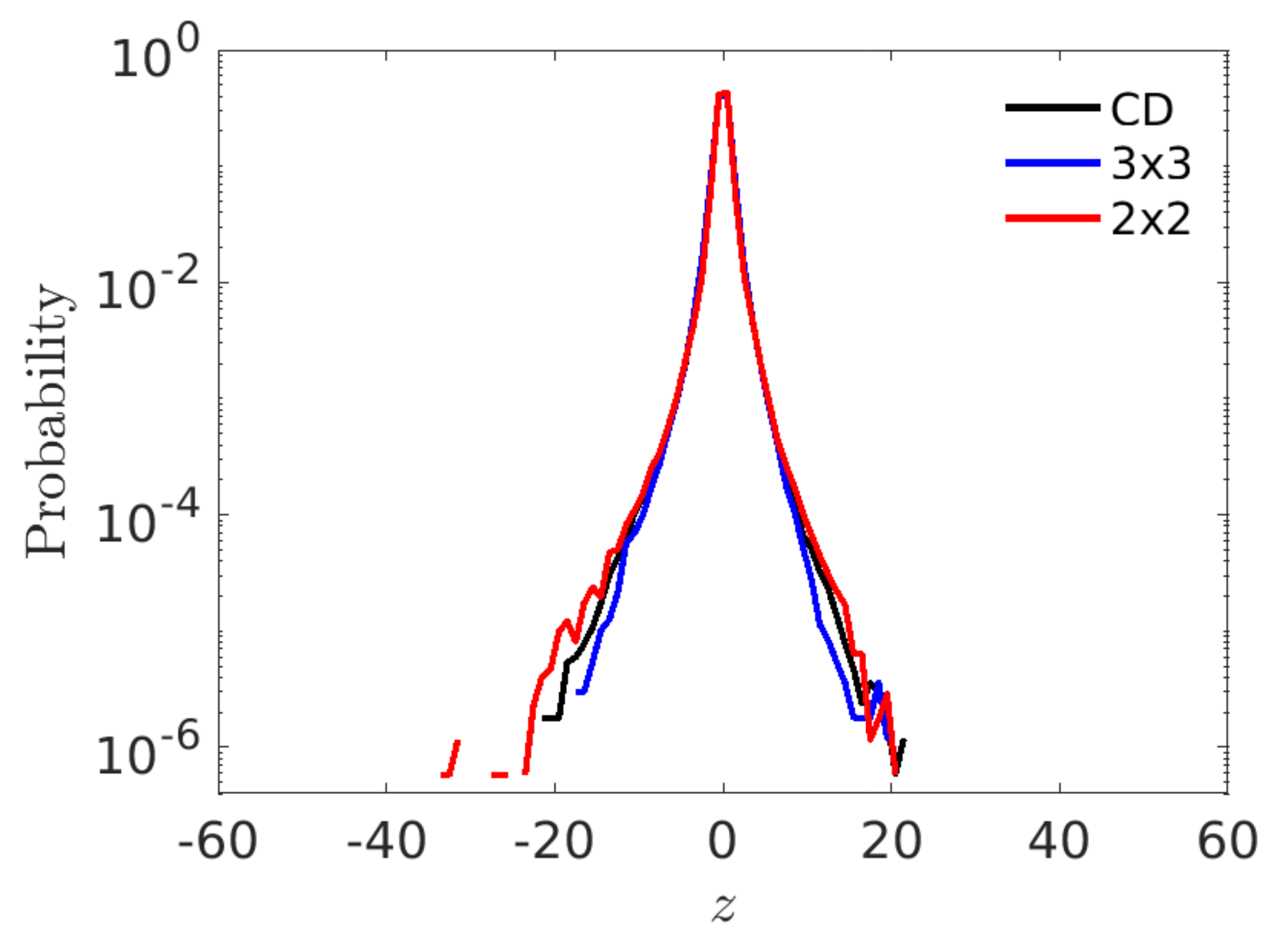
Table A1.
Comparison of first four moments of probability distribution of wind divergence obtained for standard central difference scheme (CD), and two central-difference-then-average (CDA) schemes: on a 3-by-3 block and a 2-by-2 block of WVCs.
Table A1.
Comparison of first four moments of probability distribution of wind divergence obtained for standard central difference scheme (CD), and two central-difference-then-average (CDA) schemes: on a 3-by-3 block and a 2-by-2 block of WVCs.
| Statistic | CD | CDA 3-by-3 | CDA 2-by-2 |
|---|---|---|---|
| Mean [ s] | 0.043 | 0.044 | 0.071 |
| Std. Dev. [ s] | 5.1 | 4.4 | 6.1 |
| Skewness | −0.55 | −0.41 | −0.88 |
| Kurtosis | 26 | 19 | 38 |
References
- Houze, R.A. 100 Years of Research on Mesoscale Convective Systems. Meteorol. Monogr. 2018, 59, 17.1–17.54. [Google Scholar] [CrossRef]
- Tomassini, L. The Interaction between Moist Convection and the Atmospheric Circulation in the Tropics. Bull. Am. Meteorol. Soc. 2020, 101, E1378–E1396. [Google Scholar] [CrossRef] [Green Version]
- Belmonte Rivas, M.; Stoffelen, A. Characterizing ERA-Interim and ERA5 surface wind biases using ASCAT. Ocean Sci. 2019, 15, 831–852. [Google Scholar] [CrossRef] [Green Version]
- Stoffelen, A.; Vogelzang, J.; Marseille, G. High resolution data assimilation guide (version 1.2). In Eumetsat Nwp SAF Report Nwpsaf-KN-UD-008; KNMI: De Bilt, The Netherlands, 2018. [Google Scholar]
- Biggerstaff, M.I.; Houze, R.A. Kinematic and Precipitation Structure of the 10–11 June 1985 Squall Line. Mon. Weather. Rev. 1991, 119, 3034–3065. [Google Scholar] [CrossRef]
- Portabella, M.; Stoffelen, A.; Lin, W.; Turiel, A.; Verhoef, A.; Verspeek, J.; Ballabrera-Poy, J. Rain effects on ASCAT retrieved winds: Towards an improved quality control. IEEE Trans. Geosci. Remote Sens. 2012, 50, 2495–2506. [Google Scholar] [CrossRef]
- Lin, W.; Portabella, M.; Stoffelen, A.; Verhoef, A.; Turiel, A. ASCAT Wind Quality Control Near Rain. IEEE Trans. Geosci. Remote Sens. 2015, 53, 4165–4177. [Google Scholar] [CrossRef] [Green Version]
- Lin, W.; Portabella, M.; Stoffelen, A.; Vogelzang, J.; Verhoef, A. ASCAT wind quality under high subcell wind variability conditions. J. Geophys. Res. Ocean. 2015, 120, 5804–5819. [Google Scholar] [CrossRef] [Green Version]
- Kilpatrick, T.J.; Xie, S.P. ASCAT observations of downdrafts from mesoscale convective systems. Geophys. Res. Lett. 2015, 42, 1951–1958. [Google Scholar] [CrossRef]
- Priftis, G.; Lang, T.J.; Chronis, T. Combining ASCAT and NEXRAD Retrieval Analysis to Explore Wind Features of Mesoscale Oceanic Systems. J. Geophys. Res. Atmos. 2018, 123, 10341–10360. [Google Scholar] [CrossRef]
- Garg, P.; Nesbitt, S.W.; Lang, T.J.; Priftis, G.; Chronis, T.; Thayer, J.D.; Hence, D.A. Identifying and Characterizing Tropical Oceanic Mesoscale Cold Pools using Spaceborne Scatterometer Winds. J. Geophys. Res. Atmos. 2020, 125, e2019JD031812. [Google Scholar] [CrossRef]
- Priftis, G.; Lang, T.J.; Garg, P.; Nesbitt, S.W.; Lindsley, R.D.; Chronis, T. Evaluating the Detection of Mesoscale Outflow Boundaries Using Scatterometer Winds at Different Spatial Resolutions. Remote Sens. 2021, 13, 1334. [Google Scholar] [CrossRef]
- Xu, X.; Stoffelen, A. Improved Rain Screening for Ku-Band Wind Scatterometry. IEEE Trans. Geosc. Remote Sens. 2020, 58, 2494–2503. [Google Scholar] [CrossRef]
- Giannetti, F.; Reggiannini, R.; Moretti, M.; Adirosi, E.; Baldini, L.; Facheris, L.; Antonini, A.; Melani, S.; Bacci, G.; Petrolino, A.; et al. Real-Time Rain Rate Evaluation via Satellite Downlink Signal Attenuation Measurement. Sensors 2017, 17, 1864. [Google Scholar] [CrossRef]
- Alpers, W.; Zhang, B.; Mouche, A.; Zeng, K.; Chan, P.W. Rain footprints on C-band synthetic aperture radar images of the ocean - Revisited. Remote Sens. Environ. 2016, 187, 169–185. [Google Scholar] [CrossRef]
- Vogelzang, J.; Stoffelen, A.; Verhoef, A.; Figa-Saldana, J. On the quality of high-resolution scatterometer winds. J. Geophys. Res. 2011, 116, C10033. [Google Scholar] [CrossRef] [Green Version]
- Xu, X.; Stoffelen, A.; Meirink, J.F. Comparison of Ocean Surface Rain Rates From the Global Precipitation Mission and the Meteosat Second-Generation Satellite for Wind Scatterometer Quality Control. IEEE J. Sel. Topics Appl. Earth Observ. Remote Sens. 2020, 13, 2173–2182. [Google Scholar] [CrossRef]
- King, G.; Lin, W.; Portabella, M.; Stoffelen, A. Correlating Extremes in Wind and Stress Divergence with Extremes in Rain over the Tropical Atlantic; Science Report, OSI SAF AVS15 02; 2017. Available online: https://osi-saf.eumetsat.int/community/stories/correlating-extremes-wind-and-stress-divergence-extremes-rain-over-tropical (accessed on 15 January 2022).
- Martius, O.; Pfahl, S.; Chevalier, C. A global quantification of compound precipitation and wind extremes. Geophys. Res. Lett. 2016, 43, 7709–7717. [Google Scholar] [CrossRef] [Green Version]
- Zscheischler, J.; Naveau, P.; Martius, O.; Engelke, S.; Raible, C.C. Evaluating the dependence structure of compound precipitation and wind speed extremes. Earth Syst. Dyn. 2021, 12, 1–16. [Google Scholar] [CrossRef]
- Figa-Saldaña, J.; Wilson, J.; Attema, E.; Gelsthorpe, R.; Drinkwater, M.; Stoffelen, A. The advanced scatterometer (ASCAT) on the meteorological operational (MetOp) platform: A follow on for the European wind scatterometers. Can. J. Remote Sens. 2002, 28, 404–412. [Google Scholar] [CrossRef]
- de Kloe, J.; Stoffelen, A.; Verhoef, A. Improved use of scatterometer measurements by using stress-equivalent reference winds. IEEE J. Sel. Topics Appl. Earth Observ. Remote Sens. 2017, 10, 2340–2347. [Google Scholar] [CrossRef]
- Hersbach, H. Comparison of C-Band Scatterometer CMOD5.N Equivalent Neutral Winds with ECMWF. J. Atmos. Ocean. Technol. 2009, 27, 721–736. [Google Scholar] [CrossRef]
- Stoffelen, A.; Verspeek, J.A.; Vogelzang, J.; Verhoef, A. The CMOD7 Geophysical Model Function for ASCAT and ERS Wind Retrievals. J. Sel. Topics Appl. Earth Observ. Remote Sens. 2017, 10, 2123–2134. [Google Scholar] [CrossRef]
- Vogelzang, J.; Stoffelen, A.; Verhoef, A.; de Vries, J.; Bonekamp, H. Validation of two-dimensional variational ambiguity removal on SeaWinds scatterometer data. J. Atmos. Oceanic Technol. 2009, 26, 1229–1245. [Google Scholar] [CrossRef]
- Aminou, D. MSG’s SEVIRI instrument. ESA Bulletin 2002, 111, 15–17. Available online: https://www.esa.int/esapub/bulletin/bullet111/chapter4_bul111.pdf (accessed on 15 January 2022).
- Schmetz, J.; Pili, P.; Tjemkes, S.; Just, D.; Kerkmann, J.; Rota, S.; Ratier, A. An introduction to Meteosat Second Generation (MSG). Bull. Am. Meteorol. Soc. 2002, 83, 977–992. [Google Scholar] [CrossRef]
- Roebeling, R.A.; Holleman, I. SEVIRI rainfall retrieval and validation using weather radar observations. J. Geophys. Res. Atmos. 2009, 114, D21202. [Google Scholar] [CrossRef]
- Wolters, E.L.A.; van den Hurk, B.J.J.M.; Roebeling, R.A. Evaluation of rainfall retrievals from SEVIRI reflectances over West Africa using TRMM-PR and CMORPH. Hydrol. Earth Syst. Sci. 2011, 15, 437–451. [Google Scholar] [CrossRef] [Green Version]
- MSG-CPP: Clouds, Radiation and Precipitation from Meteosat, KNMI. Available online: https://msgcpp.knmi.nl (accessed on 12 February 2022).
- Waliser, D.E.; Gautier, C. A Satellite-derived Climatology of the ITCZ. J. Clim. 1993, 6, 2162–2174. [Google Scholar] [CrossRef]
- Houchi, K.; Stoffelen, A.; Marseille, G.J.; De Kloe, J. Statistical Quality Control of High-Resolution Winds of Different Radiosonde Types for Climatology Analysis. J. Atmos. Ocean. Technol. 2015, 32, 1796–1812. [Google Scholar] [CrossRef]
- Vogelzang, J.; Stoffelen, A. Quadruple collocation analysis of in-situ, scatterometer, and NWP winds. J. Geophys. Res. Ocean. 2021, 126, e2021JC017189. [Google Scholar] [CrossRef]
- Williams, C.R.; Ecklund, W.L.; Gage, K.S. Classification of Precipitating Clouds in the Tropics Using 915-MHz Wind Profilers. J. Atmos. Ocean. Technol. 1995, 12, 996–1012. [Google Scholar] [CrossRef]
- Yuter, S.E.; Houze, R.A. Measurements of Raindrop Size Distributions over the Pacific Warm Pool and Implications for Z–R Relations. J. Appl. Meteorol. 1997, 36, 847–867. [Google Scholar] [CrossRef] [Green Version]
- Tokay, A.; Short, D.A.; Williams, C.R.; Ecklund, W.L.; Gage, K.S. Tropical Rainfall Associated with Convective and Stratiform Clouds: Intercomparison of Disdrometer and Profiler Measurements. J. Appl. Meteorol. 1999, 38, 302–320. [Google Scholar] [CrossRef]
- Ulbrich, C.W.; Atlas, D. On the Separation of Tropical Convective and Stratiform Rains. J. Appl. Meteorol. 2002, 41, 188–195. [Google Scholar] [CrossRef]
- Penide, G.; Protat, A.; Kumar, V.V.; May, P.T. Comparison of Two Convective/Stratiform Precipitation Classification Techniques: Radar Reflectivity Texture versus Drop Size Distribution–Based Approach. J. Atmos. Ocean. Technol. 2013, 30, 2788–2797. [Google Scholar] [CrossRef]
- Liu, C.; Zipser, E.J.; Cecil, D.J.; Nesbitt, S.W.; Sherwood, S. A Cloud and Precipitation Feature Database from Nine Years of TRMM Observations. J. Appl. Meteorol. Climatol. 2008, 47, 2712–2728. [Google Scholar] [CrossRef]
- Xu, X.; Stoffelen, A. Support vector machine tropical wind speed retrieval in the presence of rain for Ku-band wind scatterometry. Atmos. Meas. Tech. 2021, 14, 7435–7451. [Google Scholar] [CrossRef]
- Vogelzang, J.; Verhoef, A. The Orientation of SeaWinds Wind Vector Cells; Technical Report, NWPSAF-KN-TR-003; EUMETSAT: Darmstadt, Germany, 2014; Available online: https://nwpsaf.eu/publications/tech_reports/nwpsaf-kn-tr-003.pdf (accessed on 15 January 2022).


Publisher’s Note: MDPI stays neutral with regard to jurisdictional claims in published maps and institutional affiliations. |
© 2022 by the authors. Licensee MDPI, Basel, Switzerland. This article is an open access article distributed under the terms and conditions of the Creative Commons Attribution (CC BY) license (https://creativecommons.org/licenses/by/4.0/).