1. Introduction
There are clear tendencies in the use of higher spatial resolution satellite sensors, both for land [
1,
2,
3] and water applications [
4]. The revisit time of these sensors has greatly improved since the launch of the two Sentinel-2 satellites. Still, in areas with frequent cloud coverage, the update frequency of cloud-free data can be considerably lower. A solution is to combine data from different missions in order to obtain more frequent observations. A combination of different sensors is also necessary when data from a sufficiently long time series are required for analysis. This is, for example, the case for agricultural monitoring in which anomaly analysis is a frequently used method to assess the agricultural production of the current growing season [
5,
6]. Combining the recent and temporally more dense Sentinel-2 data with an archive of similar datasets is then important [
5,
7]. The availability of sufficiently fine spatial resolution data with an adequate temporal frequency and sufficient spectral information is still considered as a challenge, e.g., in agricultural monitoring [
8,
9] and vegetation monitoring [
10,
11]. The use of multi-mission time series should also contribute to decrease the uncertainty in derived products [
12].
The joint use of data from different sensors raises some clear concerns about data consistency [
13,
14], and a seamless combination of EO products coming from different missions require corrections that account for the sensor differences. The Harmonized Landsat Sentinel-2 (HLS) dataset [
15] and Sen2Like tool [
16] include co-registration, the same atmospheric correction method for both sensors, bi-directional distribution function (BRDF) normalization, and correction for the differences in spectral response functions (SRF) to generate top-of-Canopy (TOC) reflectances and NDVI. Many publications exist that focus on one aspect of harmonizing data from similar sensors: radiometric gain assessment (e.g., [
17,
18,
19,
20,
21]), atmospheric correction (e.g., [
22,
23]), BRDF normalization (e.g., [
24]) and SRF correction (e.g., [
25,
26,
27,
28,
29]).
The relative importance in the consistency of the datasets for each of these corrections has not yet been explored. The evaluation of the improved consistency mainly focusses on the comparison of simultaneous acquisitions, simulations, or artificial data derived from e.g.hyperspectral images (e.g., [
25]). General statistics such as RMSE and regression analysis are often used to evaluate the performance of the harmonization measure (e.g., [
25,
26,
27]), whereas evaluation on a time series is not often performed (e.g., [
15,
23]). The evaluation is predominantly completed on TOC reflectance data or NDVI, but the impact of the harmonization measures on downstream products is not assessed.
For the Belharmony project, we considered the harmonization of a multi-sensor time series from the viewpoint of two applications: agricultural monitoring and vegetation monitoring for hydrological modelling in an urban context. The different harmonization measures were evaluated in their relative contribution to obtain more accurate and more consistent time series of NDVI and biophysical parameter fractions of absorbed photosynthetically active radiation (fAPAR), leaf area index (LAI), and fraction of vegetation cover (fCover) for these applications. We made use of the extensive set of EO data and in situ reference data which have been systematically collected over the BELAIR urban and agricultural sites. The BELAIR initiative [
30], which started in 2013, aims to develop Belgian test sites, for which targeted EO data and other measurement results are collected on behalf of the Belgian and international research communities, and which may be used as calibration and validation sites for new EO missions, data and products.
In this paper, we present a bottom-up approach where we start from the L1 TOA level of four satellite sensors: Sentinel-2A&B (S2), Landsat-8, Deimos-1 (DMC) and the center camera of PROBA-V (PV). We analyzed different causes of differences and formulated corrections for them using well-established methods. Unlike HLS [
15] and Sen2Like [
16], we started the investigation with the L1 TOA reflectance data, as differences at L1 can strongly be amplified at L2 and should therefore already be corrected for at the L1 level. Next, the impact of SRF differences was analyzed and SRF adjustment functions were proposed. A common processing chain was used to generate L2 and L3 products such that the risk of biases introduced through different algorithms (e.g., atmospheric correction) or processors was significantly reduced. BRDF normalization was not included in the processing chain, because we focused on derived biophysical parameters that were retrieved from angular reflectances. Finally, we analyzed the added value of each of the corrections on the derived L3 datasets by means of two case studies. The scientific questions that are central to this research are: (i) What is the relative impact of the harmonization measures on the data per sensor? This question includes the analysis of the relative importance of radiometric gain correction, changing the atmospheric correction to a common method for all sensors, and SRF correction on the TOC reflectances, NDVI, and downstream products. (ii) What is the impact of the harmonization measures on the accuracy of the downstream products? (iii) What is the impact of these harmonization measures on the consistency of the multi-sensor L2/L3 time series? This includes the analysis of the data between sensors and over time.
5. Discussion
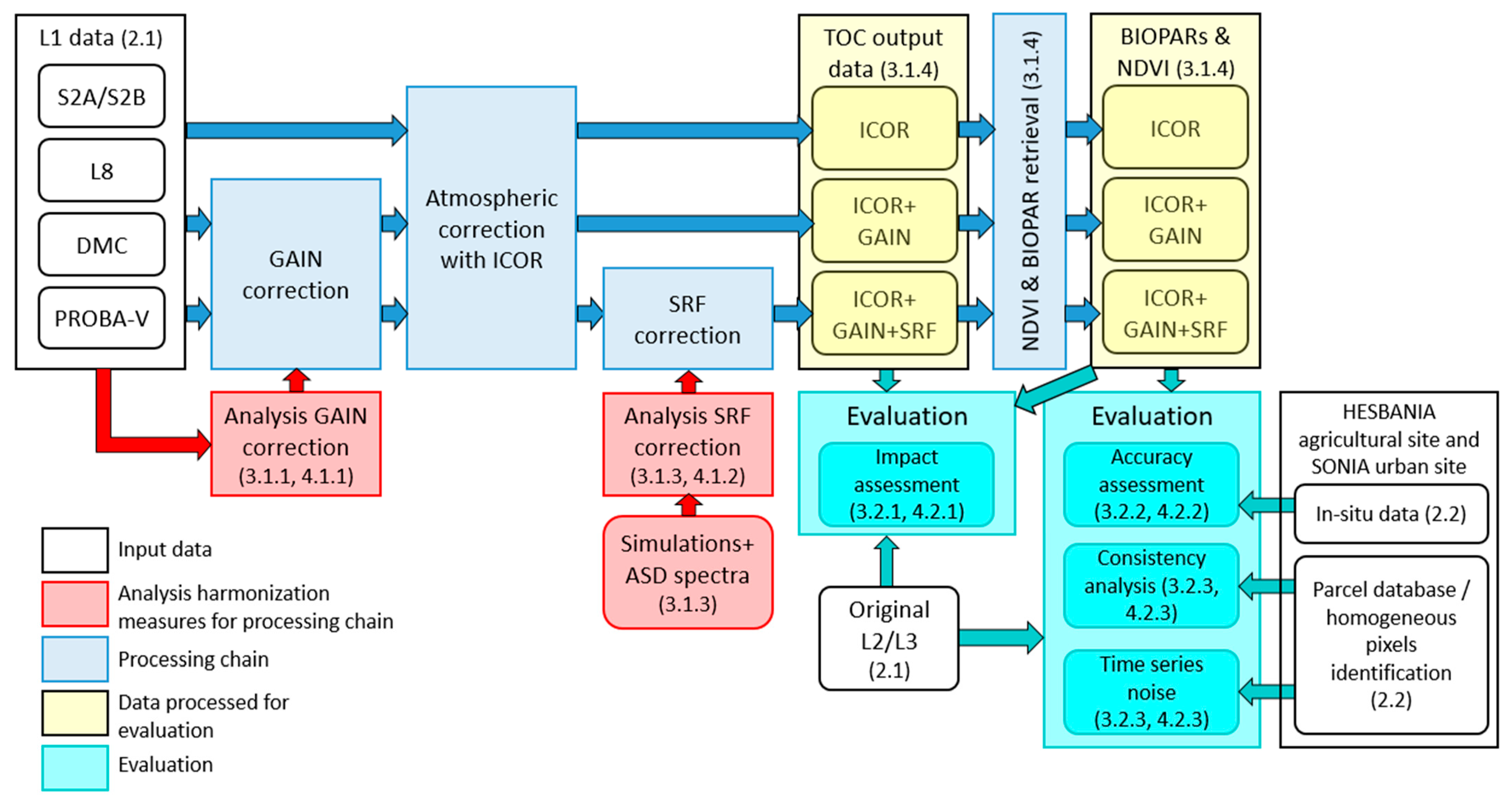
The Belharmony study was defined as a bottom-up approach from L1 to L3 products to improve consistency between S2A, S2B, L8, DMC and PV center camera, and also to analyze the relative importance of the various harmonization measures on downstream products for two applications (see
Figure 3 for overall scheme). In the study, we took S2A bands as a reference to which the differences in radiometric calibration and differences in SRF of the comparable bands of other sensors were corrected. In addition, a common processing chain was developed for all sensors including the application of the same atmospheric correction for all sensors. The different steps of the harmonization process were then evaluated on two case studies in Belgium: on an agricultural site, HESBANIA, and an urban site, SONIA.
The results of the gain correction are shown and discussed in detail in [
46]. In summary, we found inter-sensor deviations between comparable bands to be within the ±2% uncertainty range of the method applied, except for the DMC green band, where a difference of −3.5% was found. Similar results for S2 and L8 were obtained in [
17,
18,
60]. The results indicate that, with the exception of the green DMC band, a high consistency already exists between the different sensors. Nevertheless, the small differences were applied on the datasets anyway and further assessed.
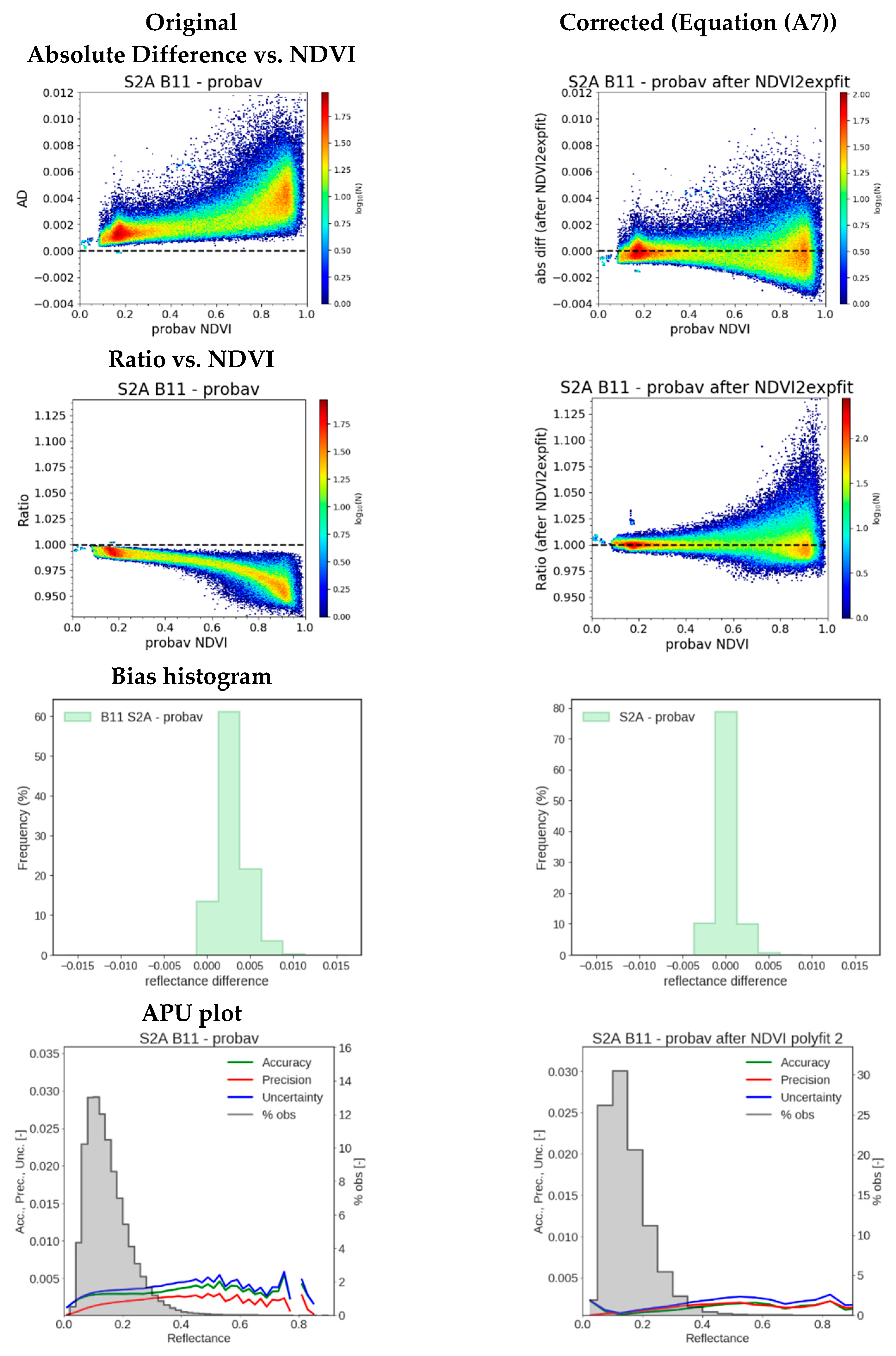
Next, correction functions for the differences in SRF were established. A large number of simulations with the addition of a set of urban spectra were used to model the differences in SRF with respect to the comparable band in S2A. Various correction functions were also estimated and evaluated on an independent dataset (APEX images). As in [
28], the optimal correction differed per sensor combination and per band. Comparing the obtained results with correction functions published in the literature is difficult, because the reference was often different (e.g., MODIS/Aqua in [
28]), or because not all sensors were part of the study, e.g., [
25] only includes S2 and none of the other sensors discussed here. For a number of sensor/band combinations, no correction was retained. This was either because both bands were already so similar that no improvement was obtained, or because the correction did not yield a significant improvement. Except for these band combinations, all other corrections functions were applied on the data for further analysis.
After processing a large set of data, different analyses were performed to evaluate the performance of the harmonization measures. These included: (1) impact assessment of the various harmonization measures on the data per sensor; (2) accuracy assessment of the downstream products using in situ data; (3) comparison of match-ups between these products from different sensors; and (4) analyses of the noise in time series generated on the combination of the different sensors.
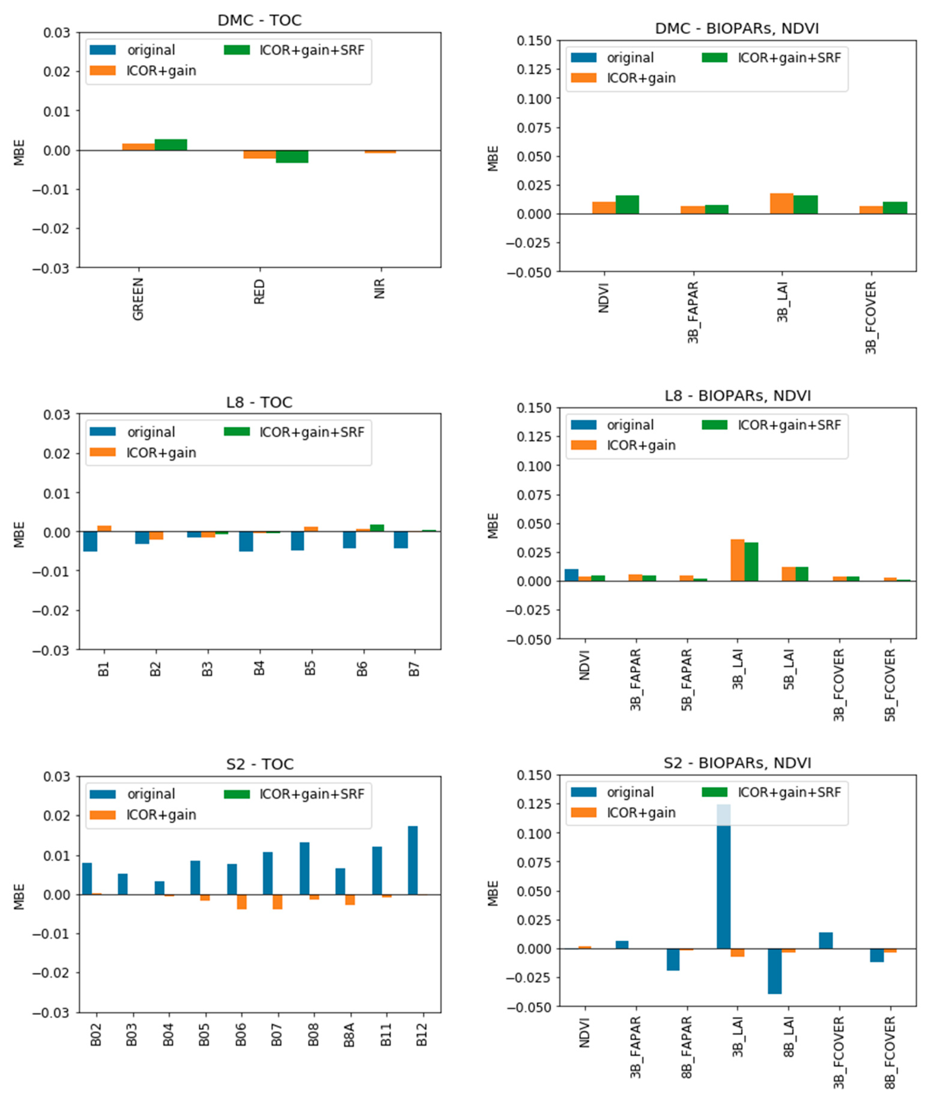
In the impact assessment of the different corrections at TOC reflectance level, we saw that the largest difference between comparable bands of the sensors was obtained when applying the same atmospheric correction instead of comparing the original data with each individual pre-processing choice. The same approach was followed in [
22] in order to increase the consistency between NOAA-AVHRR sensors and SPOT-VEGETATION. In that study, all atmospheric input data were taken from external sources and the method for atmospheric correction was the same. In the current study, the AOT was derived from the images themselves; hence, these were not the same, but estimated in a similar way. The atmospheric correction, as such, was not evaluated in this study, but is part of ACIX I and II [
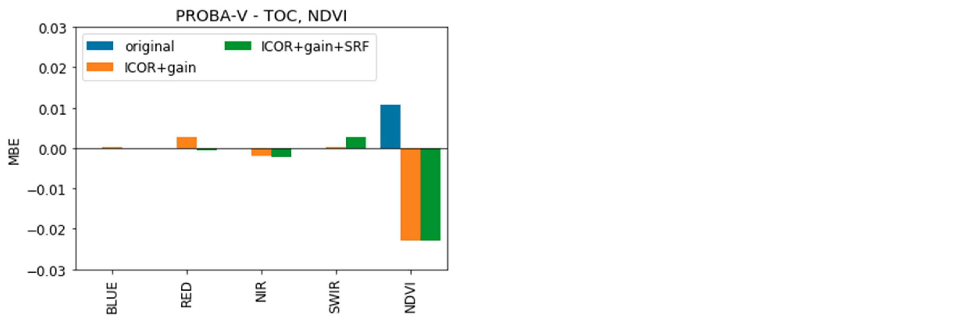
50]. The impact of the gain and SRF correction on the TOC reflectances were, in general, much smaller. Next, we looked at how these differences at TOC reflectance level translated into the derived parameters, NDVI and BIOPARs. Again, the difference was the highest when comparing the original data with ICOR data. Adding the gain and SRF corrections resulted in smaller differences with respect to the ICOR dataset.
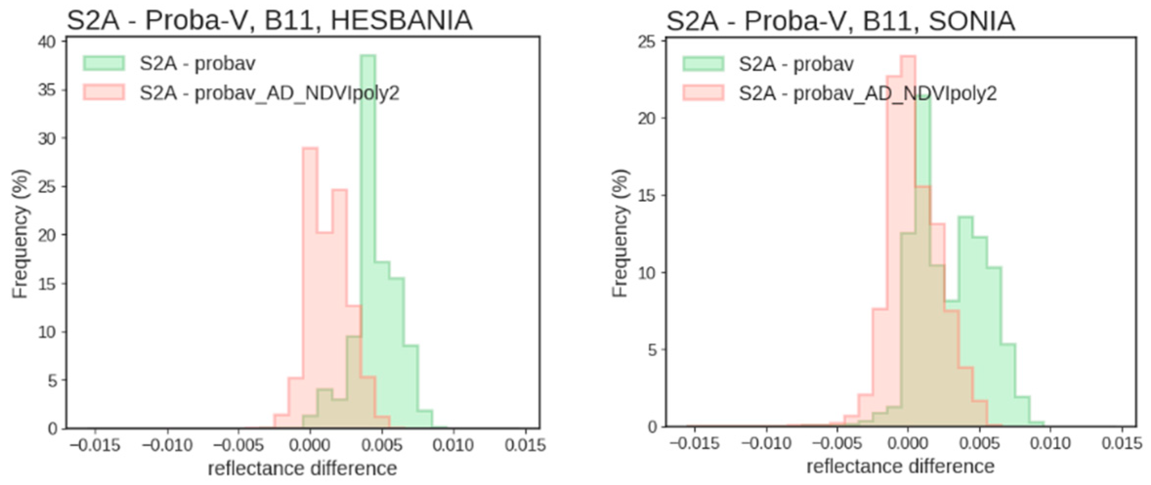
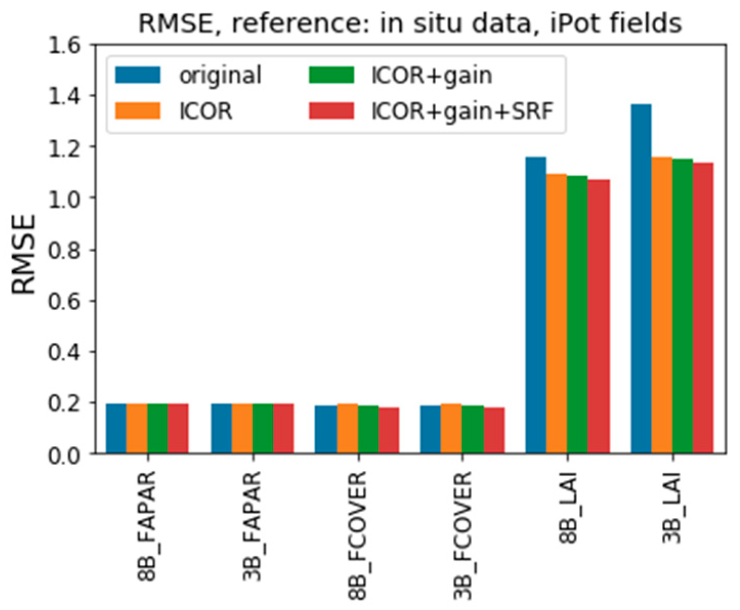
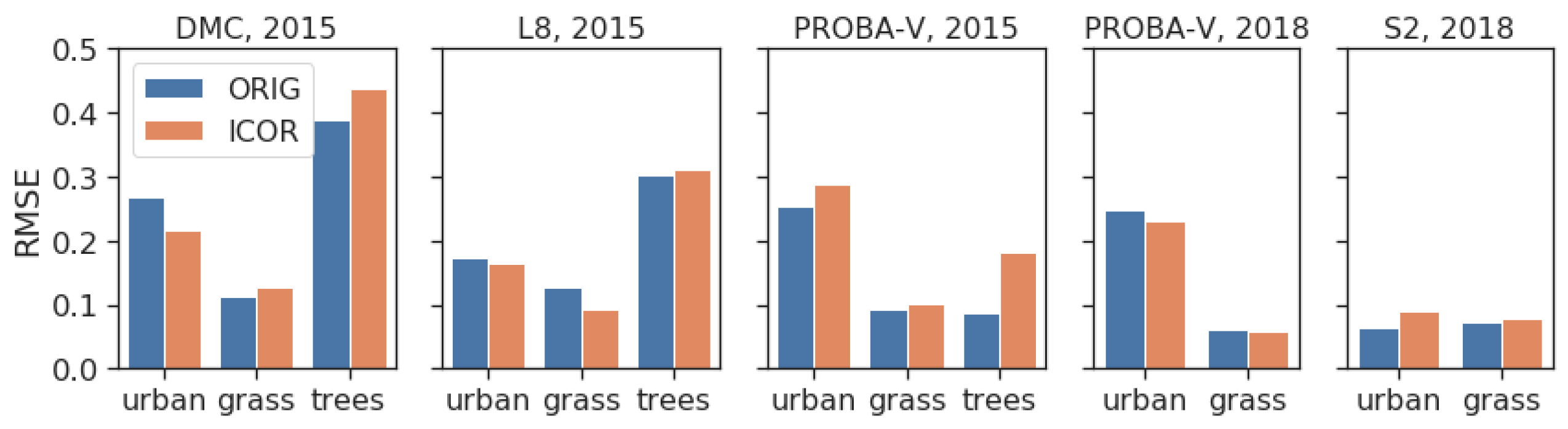
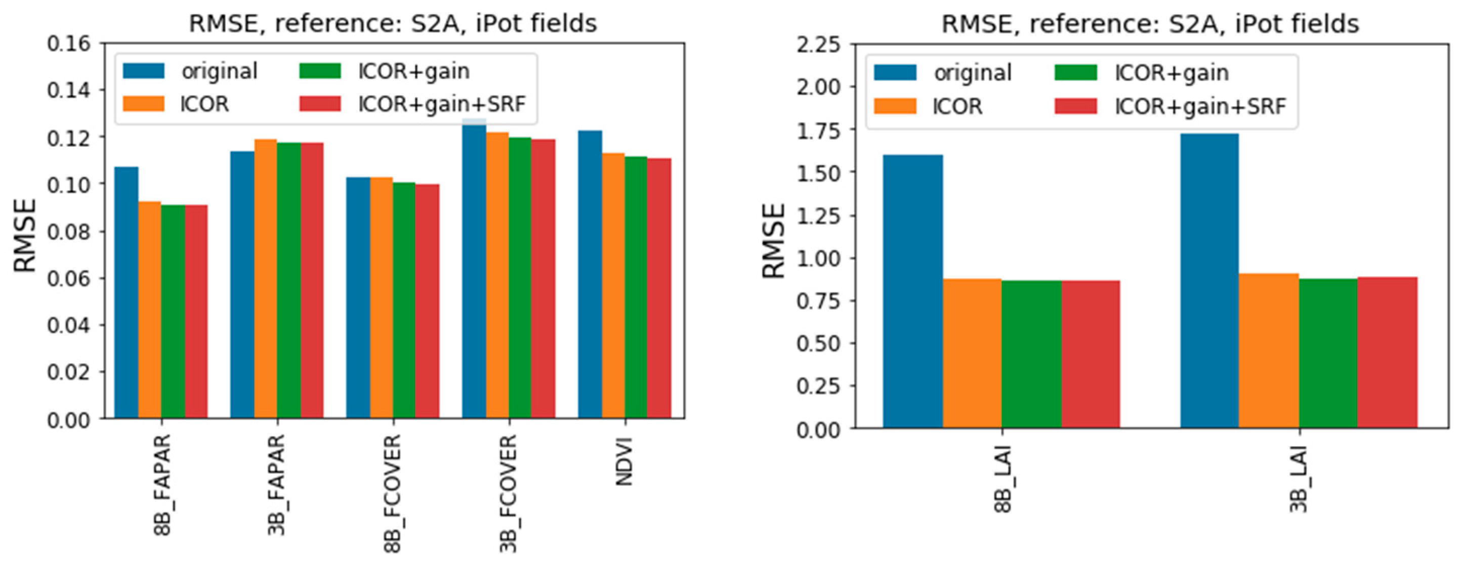
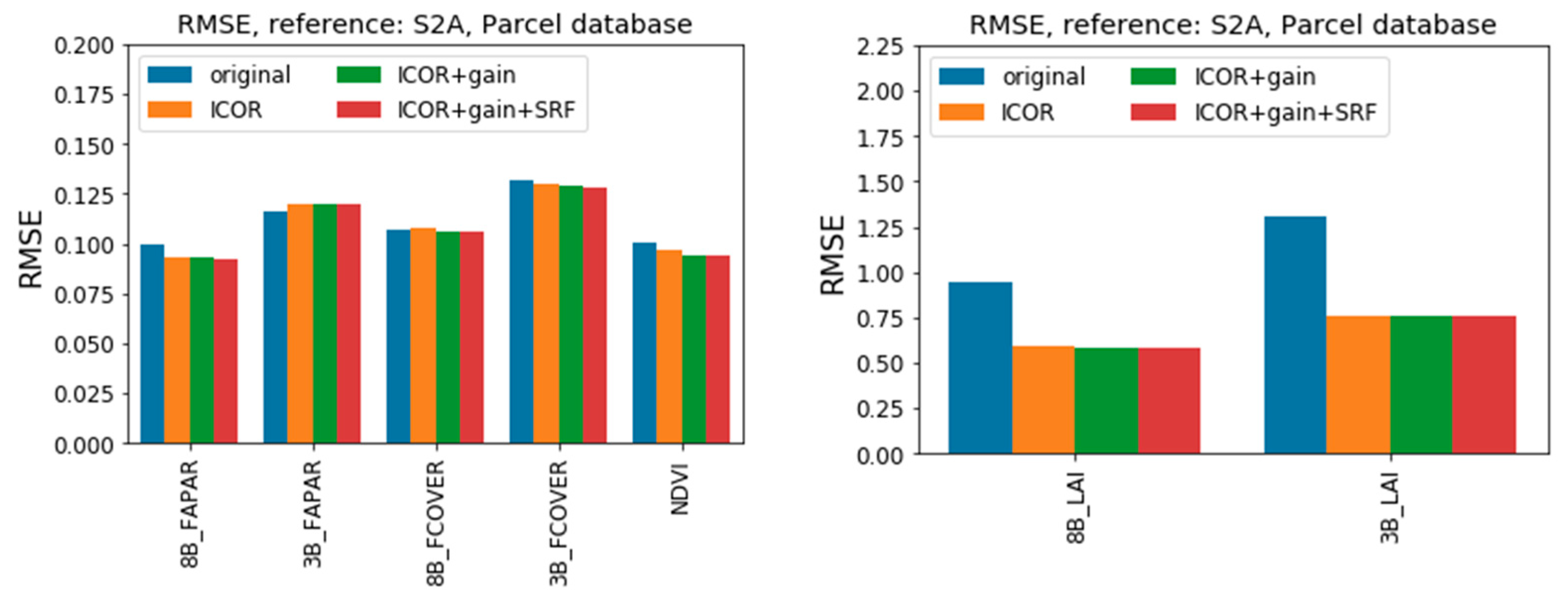
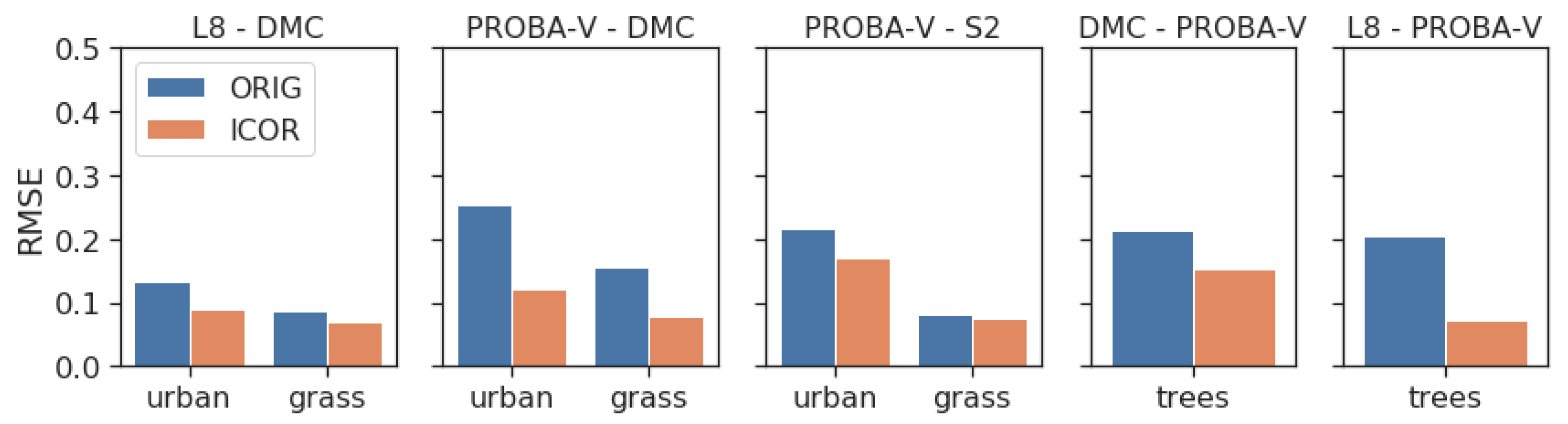
The added value of the different harmonization measures was further investigated for two distinct case study areas, in an agricultural (HESBANIA) and urban (SONIA) landscape. First, the obtained NDVI and BIOPARs generated with different corrections were validated against in situ data for these areas. The various harmonization measures did not necessarily lead to higher accuracy or precision. For LAI in HESBANIA, an agricultural site, accuracy was higher when applying the same atmospheric correction to all data sources compared to the original data. For FAPAR and FCOVER, there was only a very small difference in accuracy. For the SONIA urban site, the RMSE was higher after using the same atmospheric correction for most cases. Validation of the atmospheric correction was performed in ACIX I and II. The results of ACIX I are available in Doxani, which also includes the methods used for the original data (Sen2Cor for S2, LaSRC for L8). They demonstrate that iCOR performs almost equally as well as LaSRC for L8. On the other hand, Sen2Cor performs better than iCOR for S2. Meanwhile, some changes were made to iCOR, and these results were evaluated in ACIX II, but this study has not yet been published. The choice of iCOR was made because it can be applied to a suit of sensors.
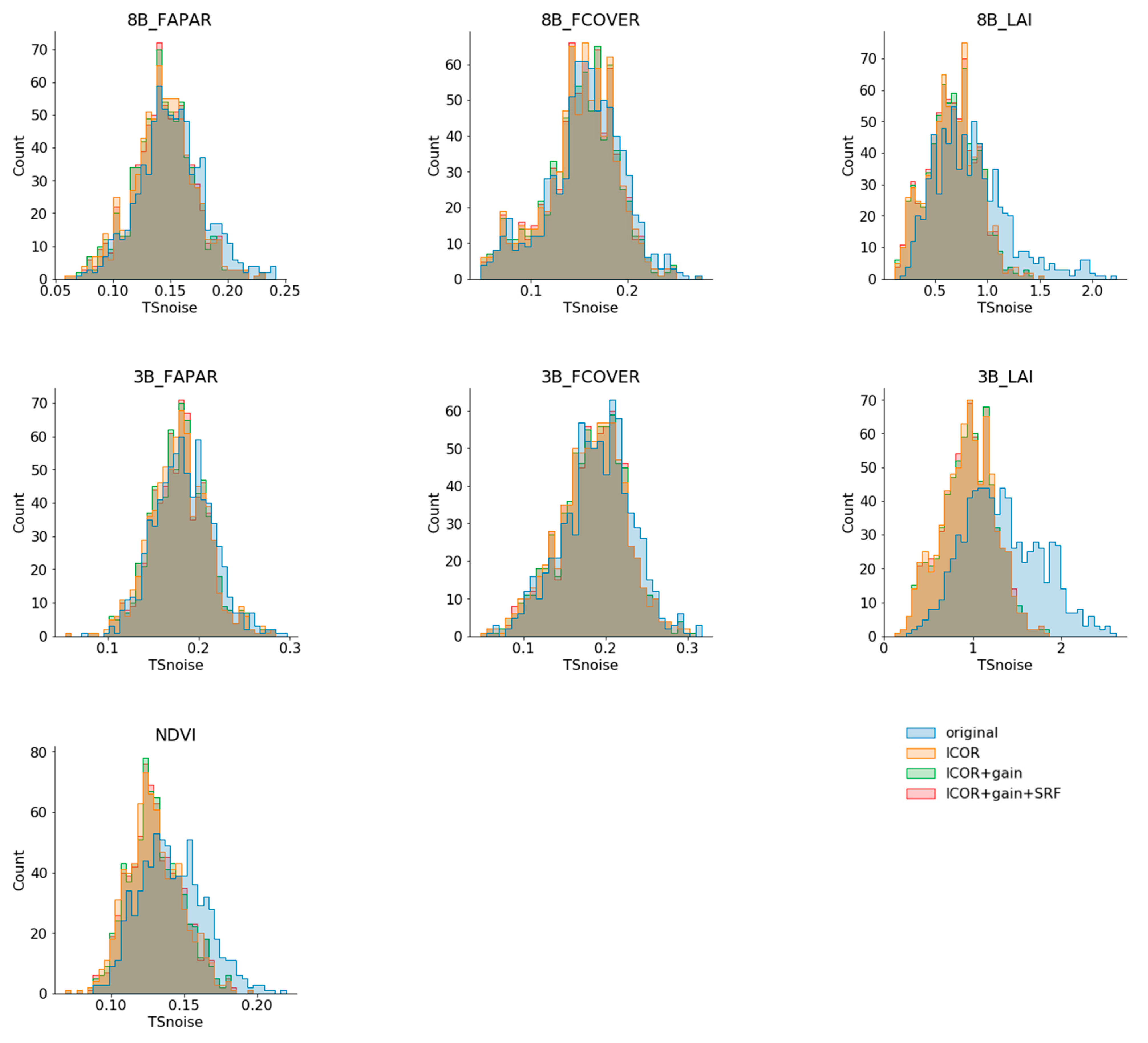
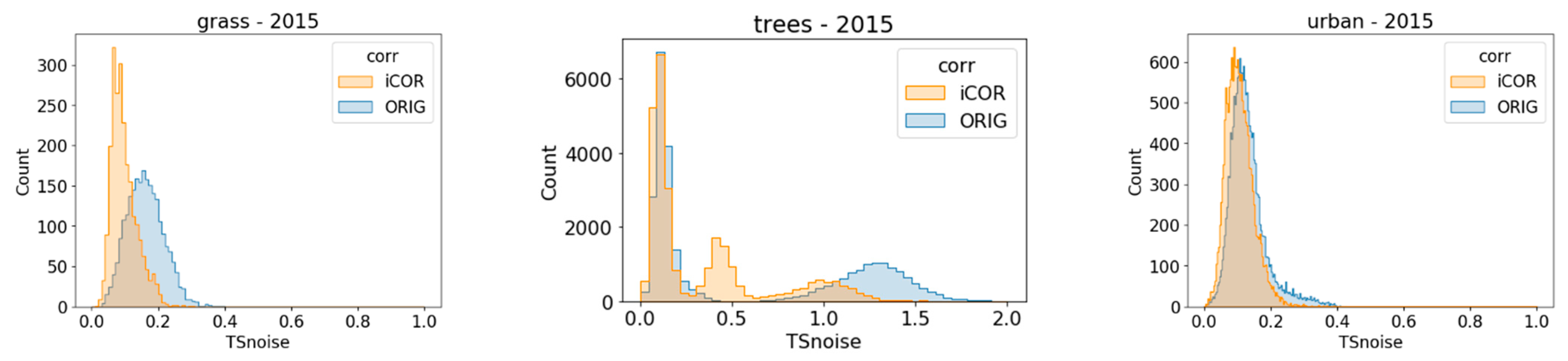
Although using iCOR did not improve the accuracy with respect to in situ data, the consistency between the datasets improved. This was demonstrated first by creating match-ups between data from one sensor and from the other sensors for the case study sites and comparing these. For both case studies, a higher consistency was found after using the same atmospheric correction. The impact of the gain and SRF corrections lead, in most cases, to a slightly higher consistency, except for FAPAR. This analysis was repeated for a large number of agricultural fields (HESBANIA) and the same results were obtained. Second, the distribution of the time series noise for the same fields in HESBANIA and for homogeneous pixels in SONIA were assessed, which confirmed the previous results that using the same atmospheric correction had the largest contribution to a better consistency between the datasets. Applying the gain and SRF correction did not result in less noise in the time series. Although the two case sites covered different land cover types, similar results for the analysis were obtained.
Accurate calibrated instruments are a prerequisite for interoperability between sensors. The reason why the gain correction did not improve the consistency is because the sensors were already well calibrated [
61,
62,
63,
64] and the remaining difference estimated was small and within the uncertainty range of the method used [
60]. The results obtained demonstrated the added value of correcting for SRF differences on a controlled dataset based on APEX images. Here, the only difference between the dataset was the SRF used to create artificial images. The added value of the SRF correction was not confirmed on the evaluation with the real sensor data. This could be because the impact was smaller than the differences that were induced by other sources such as BRDF effects in the images. The BIOPARs, however, were retrieved while considering the observation and illumination geometry, and the output should therefore already account for anisotropy effects. This was not the case for the NDVI. BRDF effects were not considered in the study and are a source of difference that have to be accounted for, as well for the generation of fully harmonized multi-mission time series [
65]. Although satellites such as S2 or L8 acquire images close to nadir, they are not likely to observe the same target over a long period of time with a unique Sun-target-sensor geometry configuration. The latter changes according to day of the year, scanning strategy, and stage in the life of the mission. Thus, an inconsistent sampling of the BRDF in time and space will inevitably introduce directional effects that can hamper with the interpretation of observed temporal changes in surface reflectance time series. Thus, to properly disentangle changes due to vegetation from those simply introduced by directional effects, the BRDF of a target must be modeled. By approximating the anisotropy of a target with a BRDF model (e.g., [
66,
67]), we can normalize (adjust) all surface reflectance observations to a common Sun-sensor geometry in order to derive consistent and smooth surface reflectance time series.
6. Conclusions
To conclude, we recall the research questions that were formulated. What is the relative impact of the harmonization measures on the data per sensor? The relative impact of the harmonization measures differed from sensor to sensor and from band to band. In general, the impact of changing the atmospheric correction to ICOR was the largest. The gain and SRF corrections had smaller impacts, and sometimes had opposite signs. A similar impact was observed for the downstream BIOPAR products.
What is the impact of the harmonization measures on the accuracy of the downstream products? The harmonization measures did not necessarily lead to a higher accuracy of the products.
What is the impact of all these harmonization measures on the consistency of the multi-sensor L2/L3 time series? Using the same atmospheric correction method especially resulted in a better agreement between the NDVI and BIOPARs, and the noise in the time series was reduced. Accurate calibration of the sensors was, of course, also important, and the fact that we did not find an added value in applying a gain correction suggests that the sensors were already closely calibrated. The SRF correction impact could not be demonstrated, probably because other sources of differences were not taken into account, such as BRDF correction.


