Research on Shore-Based River Flow Velocity Inversion Model Using GNSS-R Raw Data

Abstract

Global navigation satellite system reflectometry technology (GNSS-R) is rarely used for river flow velocity inversion, and in particular, there is currently no research using the BeiDou Navigation Satellite System reflectometry technology (BDS-R) for river flow velocity inversion. In this paper, a carrier phase observation of river flow velocity inversion model is proposed. The interference phase is the integral of the Doppler frequency. The raw intermediate frequency (IF) data sets are processed through an open-loop method to obtain the Doppler frequency observation generated by river flow and then realize velocity inversion. The shore-based river current measurement was conducted on the south bank of Dashengguan Yangtze River in Nanjing city, Jiangsu Province, for nearly two hours on 22 April 2021. After realizing the inversion of river flow velocity in GPS L1, the combined inversion of BDS B1I GEO satellite and IGSO satellite is realized for the first time, which demonstrates the feasibility of river flow velocity inversion using BDS reflected signals. Compared with the real river flow velocity, the GPS L1 PRN 4 (1st period) inversion precision reaches up to 0.028 m/s (mean absolute error, MAE) and 0.036 m/s (root mean square error, RMSE). In parallel, BDS GEO 2 inversion precision can reach 0.048 m/s (MAE) and 0.063 m/s (RMSE), and BDS IGSO 10 inversion precision is 0.061 m/s (MAE) and 0.073 m/s (RMSE). These results illustrate that satellite elevation change rate and distance between specular points and current meter may have a negative effect on the accuracy of river flow velocity inversion. Specular points obstructed by obstacles or too far from the velocity meter may introduce uncertain error in both MAE and RMSE. Neither the satellite elevation nor the signal strength has an obvious correlation with inversion precision, which is consistent with the theoretical principle.

1. Introduction

River flow velocity detection is of great significance in hydrology work. It is also an essential fundamental link in hydrologic detection, hydrologic prediction, hydrodynamic research, flood control engineering design, and ecological environment assessment [1]. Traditional river flow velocity detection methods, such as artificial detection, are work-intensive, time consuming, and inefficient. Additionally, the more extreme the hydrological situation is, the more difficult it is to measure the river flow velocity, such as during floods and typhoons [2,3].

Global navigation satellite system reflectometry technology (GNSS-R) possesses the characteristics of being global, all-weather-accessing, and low-cost. At present, GNSS-R technology has been widely used in sea surface altimetry [4,5,6], sea surface wind fields [7,8,9], sea ice sensing [10,11,12], inland water detection [13,14], sea surface oil slicks [15,16], sea surface effective wave height [17,18], and other application fields. Better yet, it still has great potential in the applications of remote sensing inversion.

As in traditional radar remote sensing, GNSS-R carrier phase observation has been widely used to measure sea surface height (SSH). Since the first lake altimetry through carrier phase observation under shore-based conditions [19], attributed to its better measurement accuracy, carrier phase observation has also been introduced for sea-level [20] and sea ice experiments [21]. Meanwhile, GNSS-R carrier phase observation altimetry has been expanded in different airborne experiments [22,23,24], and more recently, with space-borne data collected by the U.K.’s TechDemoSat-1 (TDS-1) [25,26] and NASA’s Cyclone GNSS (CYGNSS) missions [27,28]. Based on the carrier phase observations, a different method for deriving Doppler observations is proposed and applied to altimetry [29]. In 2015, Weihua Bai et al. published a new potential application of GNSS-R through carrier phase observation [30], inversion of river flow velocity, and verified its feasibility by using GPS L1 satellite reflected signals, with MAE reaching 0.0271 m/s. However, the inversion lasted for only minutes, without further systematic analysis of the accuracy and principle of river flow velocity inversion. Above all, few experiments are using GNSS-R technology to detect river flow velocity, and in particular, there is no research on river flow velocity inversion currently using BeiDou Navigation Satellite System reflectometry technology (BDS-R).

BDS consists of geosynchronous orbit (GEO) satellites, inclined geosynchronous orbit (IGSO) satellites, and medium orbit (MEO) satellites. The GEO satellites have low angular velocity and almost no change in elevation. Their maximum speed is between 80 m/s and 90 m/s. The trajectory of an IGSO satellite is in the shape of “8”, and the elevation potentially changes at a considerable rate. The maximum speed will reach about 2800 m/s. The maximum velocity of an MEO satellite is about 3780 m/s. For BDS receivers under shore-based experimental conditions, the full Doppler frequency shift of BDS GEO/IGSO/MEO satellites are 70.8 Hz, 2207.4 Hz, and 4496.5 Hz, respectively [31].

Here, the combination of B1I GEO satellite and IGSO satellite of BDS is used to carry out river flow velocity inversion for the first time. GPS/BDS dual-mode GNSS-R detection equipment was used to obtain the raw IF data of GPS L1/BDS B1I direct and reflected signals in the actual experiment. Meanwhile, self-developed soft receiver process data was used to obtain Doppler frequency extracted by interferometric carrier phase and realize river flow inversion. Finally, the velocity inversion results are compared with the actual velocity, and the influence of satellite elevation angle change rate and satellite signal intensity on the accuracy of river flow velocity inversion is further explored.

2. River Flow Velocity Inversion Model

The GNSS-R carrier phase river flow velocity model includes two essential parts: the open-loop tracking method and carrier phase river flow velocity inversion method. The former is used to obtain the interferometric carrier phase observation between direct signals and reflected signals and to extract the Doppler frequency, and the latter is used to conduct river flow velocity inversion.

2.1. GNSS-R Reiver Velocity Inversion Process

Under the shore-based experimental conditions, it could be assumed that the river flow velocity of the target area is a fixed vector over a short time. Therefore, velocity inversion results are calculated every two minutes in this paper. The whole inversion process includes three steps:

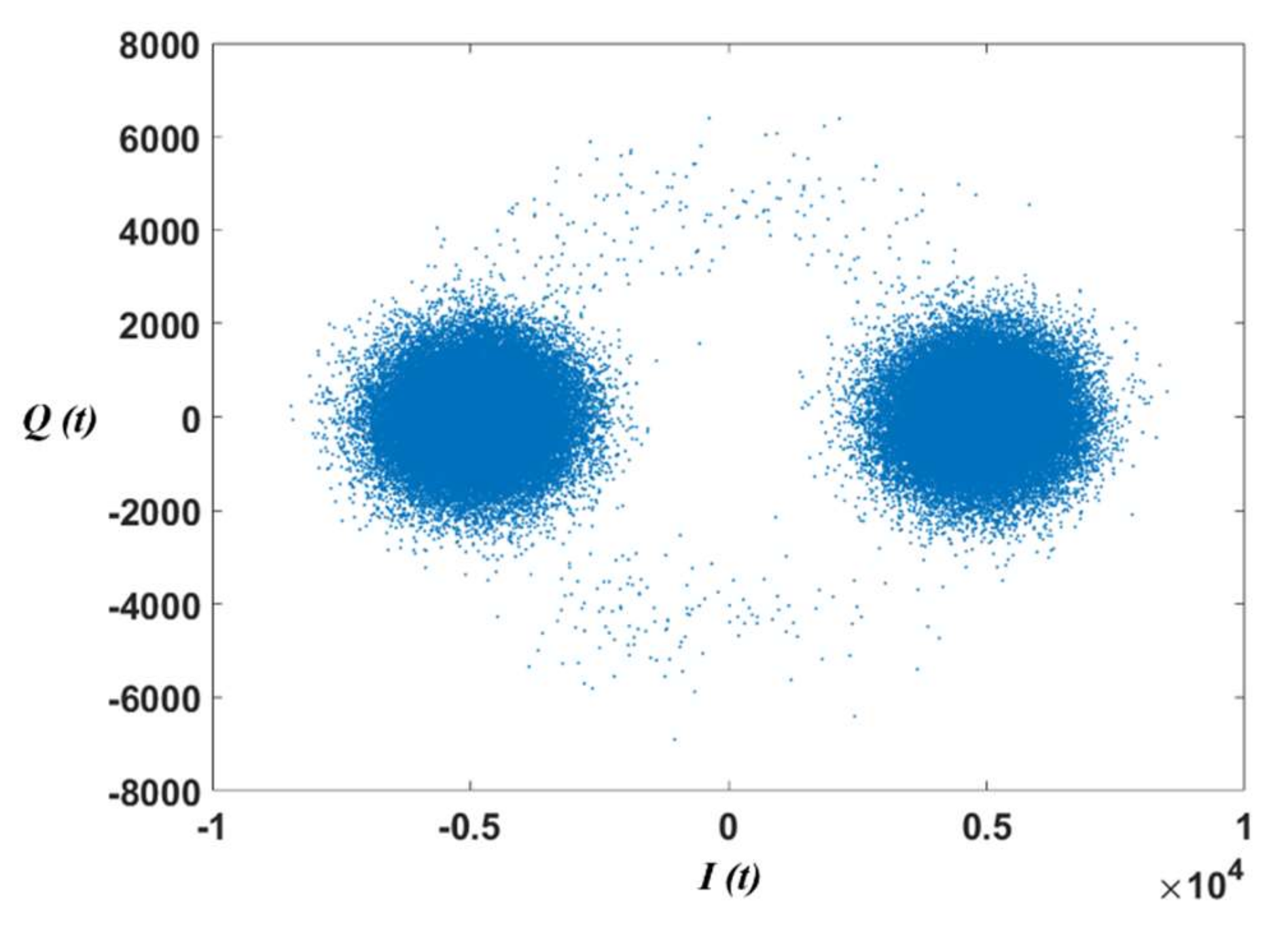
First of all, by preprocessing to remove corrupted raw IF data, the Lissajous figure is used to judge the multi-frequency relationship and phase difference between two waveform signals (I branch, Q branch) in the field of signal processing. It plays an important role in regulating the signal-tracking loop [31]. In addition, the Lissajous figure is also used as a criterion for judging whether the carrier phase replica ${\phi }_{Local}$ could take the place of the direct signal carrier phase ${\phi }_{direct}\left(t\right)$. Figure 1 is the Lissajous figure of the GPS PRN 9 for 2 min on 22 April 2021, 10:40 am−10:42 a.m. local time (LT).

Figure 1. The Lissajous figure of the GPS PRN 9 direct signal in 2 min.

Then, in the data processing stage, the residual phase ${\phi }_{raw}$ is obtained by processing the raw IF data. The details of processing raw IF data and how to obtain ${\phi }_{out}$ will be introduced in Section 2.2. After further processing of fast Fourier transform (FFT) data, the flow rate $V_{flow}$ is inverted. The method of obtaining the Doppler frequency from the interferometric phase and using the river inversion model for inversion is introduced in Section 2.3. During the experiment, the average river flow velocity $V_{real}$ was recorded every 5 min in the experimental area using a contact current meter. The current meter model is H-ADCP CM300, and the system frequency is 300 kHz, which calculates the flow velocity by analyzing the frequency shift of the Doppler.

Eventually, the inversion river flow velocity $V_{flow}$ is compared with the real velocity $V_{real}$ to verify the precision and conduct further error analysis. Figure 2 is the flowchart of the GNSS-R river flow velocity inversion method.

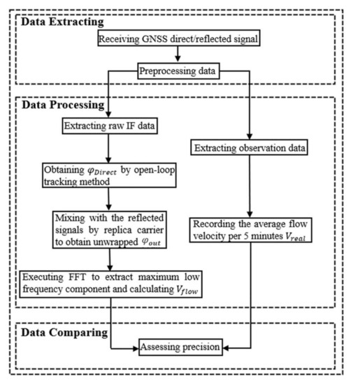
Figure 2. Flow chart of stream velocity inversion method.

2.2. Signal Open-Loop Tracking Method

For the shore-based Yangtze River experiment, separated direct and reflecting antennas were used. The receiver provides direct and reflected samples at 20 MHz to GNSS signals and then generates raw IF data of GNSS signals. The direct sampling applies the open-loop tracking method to adjust Doppler frequency and carrier phase by soft receiver (direct carrier replica). The cosine carrier and sine carrier generated by the local carrier numerically controlled oscillator (NCO) can be expressed as follows:

$$\begin{array}{c}{\mathit{v}}_{\mathit{I}}(t)=\cos ({\phi }_{\mathit{Local}}(t)+{\phi }_{\mathit{l}0})\\ {\mathit{v}}_{\mathit{Q}}(t)=\sin ({\phi }_{\mathit{Local}}(t)+{\phi }_{\mathit{l}0})\end{array}$$

(1)

where ${\phi }_{Local}\left(t\right)$ and ${\phi }_{l0}$ represent the carrier phase and initial phase of the direct signal, respectively. When the tracking loop enters a stable tracking state, the difference between the direct signal carrier and carrier replication frequency is 0, the carrier phase difference is close to 0, and the code phase difference is within 0.01–0.1 code chip [32]. The GNSS signal is a quasi-monochromatic and phase-modulated spherical wave signal [33], whose reflected signal can be expressed as follows:

$${\mathit{u}}_{\mathit{r}}(t)={\mathit{C}}_{\mathit{r}}(t)\cdot {\mathit{D}}_{\mathit{r}}(t)\cdot {\mathit{A}}_{\mathit{r}}(t).\cos ({\phi }_{\mathit{Reflect}}(t)+{\phi }_{r0})$$

(2)

where $C_r\left(t\right)$ represents pseudo-random code, $D_r\left(t\right)$ is navigation bit, $A_r\left(t\right)$ is reflected signal’s amplitude, and ${\phi }_{Reflect}\left(t\right)$ and ${\phi }_{r0}$ represent the carrier phase and initial phase of the reflected signal, respectively. The correlation operation between sine and cosine carrier replica and the reflected signal can be defined as follows [34]:

$$\begin{array}{c}{\mathit{I}}_{\mathit{n}}=\frac{1}{{\mathit{T}}_{\mathit{coh}}}{\displaystyle {\int }_{{\mathit{t}}_{\mathit{n}}}^{{\mathit{t}}_{\mathit{n}}+{\mathit{T}}_{\mathit{coh}}}{\mathit{u}}_{\mathit{r}}(t)}\cdot {\mathit{V}}_{\mathit{I}}(t)+{\mathit{N}}_{\mathit{i}}\\ \approx \overline{{\mathit{A}}_{\mathit{n}}}\cdot \mathrm{sinc}(2\pi \overline{\Delta {\mathit{f}}_{\mathit{n}}}\cdot {\mathit{T}}_{\mathit{coh}})\cdot \cos (2\pi \overline{\Delta {\mathit{f}}_{\mathit{n}}}\cdot {\mathit{T}}_{\mathit{coh}}+\Delta \varphi )+{\mathit{N}}_{\mathit{i}}\\ {\mathit{Q}}_{\mathit{n}}=\frac{1}{{\mathit{T}}_{\mathit{coh}}}{\displaystyle {\int }_{{\mathit{t}}_{\mathit{n}}}^{{\mathit{t}}_{\mathit{n}}+{\mathit{T}}_{\mathit{coh}}}{\mathit{u}}_{\mathit{r}}(t)}\cdot {\mathit{V}}_{\mathit{Q}}(t)+{\mathit{N}}_{\mathit{q}}\\ \approx \overline{{\mathit{A}}_{\mathit{n}}}\cdot \mathrm{sinc}(2\pi \overline{\Delta {\mathit{f}}_{\mathit{n}}}\cdot {\mathit{T}}_{\mathit{coh}})\cdot \sin (2\pi \overline{\Delta {\mathit{f}}_{\mathit{n}}}\cdot {\mathit{T}}_{\mathit{coh}}+\Delta \varphi )+{\mathit{N}}_{\mathrm{q}}\end{array}$$

(3)

where $T_{coh}$ (1 ms in this paper) is the coherence integration time and is generally an integer multiple of 1 ms, $sinc\left(x\right)=\sin \left(x\right)/x$. $\overline{\Delta f}=f_{Reflect}-f_{Local}$ refers to the frequency difference between the carrier replica and the input reflected signal in the coherent time, $\Delta \varphi$ is the initial phase difference between the carrier replica and the input reflected signal, and $N_i$ and $N_q$ represent the random noise of I and Q components, respectively. The subscript $n$ is time t, $t_n$<$t$<$t_n$+$T_{coh}$.

In the derivation of the above equation, the following assumption is made [35]: the coherence integral $T_{coh}$ is long enough for the high-frequency (replica carrier frequency plus reflected signal carrier frequency) components of I and Q to be filtered by the integrator. For this reason, Equations (4) and (5) reasonably omit the sum frequency (high-frequency) component in derivation, and the corresponding, approximately equal, sign appears.

Under the circumstances of the shore-based experiment, when signals enter the carrier tracking stage, the frequency difference between input reflected signal and local carrier replica has been very close. It has generally been much smaller than the integrator’s bandwidth, ∆f ≪1/$T_{coh}$, so I and Q components can be approximated as follows:

$$\begin{array}{l}{\mathit{I}}_{\mathit{n}}=\overline{{\mathit{A}}_{\mathit{n}}}\cdot \cos (2\pi \overline{\Delta {\mathit{f}}_{\mathit{n}}}\cdot {\mathit{T}}_{\mathit{coh}}+\Delta \varphi ))+{\mathit{N}}_{\mathit{i}}\\ {\mathit{Q}}_{\mathit{n}}=\overline{{\mathit{A}}_{\mathit{n}}}\cdot \sin (2\pi \overline{\Delta {\mathit{f}}_{\mathit{n}}}\cdot {\mathit{T}}_{\mathit{coh}}+\Delta \varphi )+{\mathit{N}}_{\mathit{q}}\end{array}$$

(4)

Equations (5) and (6) could be defined as the following complex vector form:

$${\mathit{r}}_{\mathit{n}}={\mathit{I}}_{\mathit{n}}+j{\mathit{Q}}_{\mathit{n}}=\overline{{\mathit{A}}_{\mathit{n}}}\cdot e^{j(\Delta {\varphi }_n)}$$

(5)

Vector amplitude $A_n$ and raw residual phase ${\phi }_{out}$ can be defined as follows:

$$\begin{array}{c}\overline{{\mathit{A}}_{\mathit{n}}}=\sqrt{{\mathit{I}}_{\mathit{n}}^2+{\mathit{Q}}_{\mathit{n}}^2}\\ {{\displaystyle \phi }}_{\mathit{out}}^{\mathit{n}}=\arctan 2(\frac{{\mathit{Q}}_{\mathit{n}}}{{\mathit{I}}_{\mathit{n}}})=2\pi \overline{\Delta {\mathit{f}}_{\mathit{n}}}\cdot {\mathit{T}}_{\mathit{coh}}+\Delta \varphi \end{array}$$

(6)

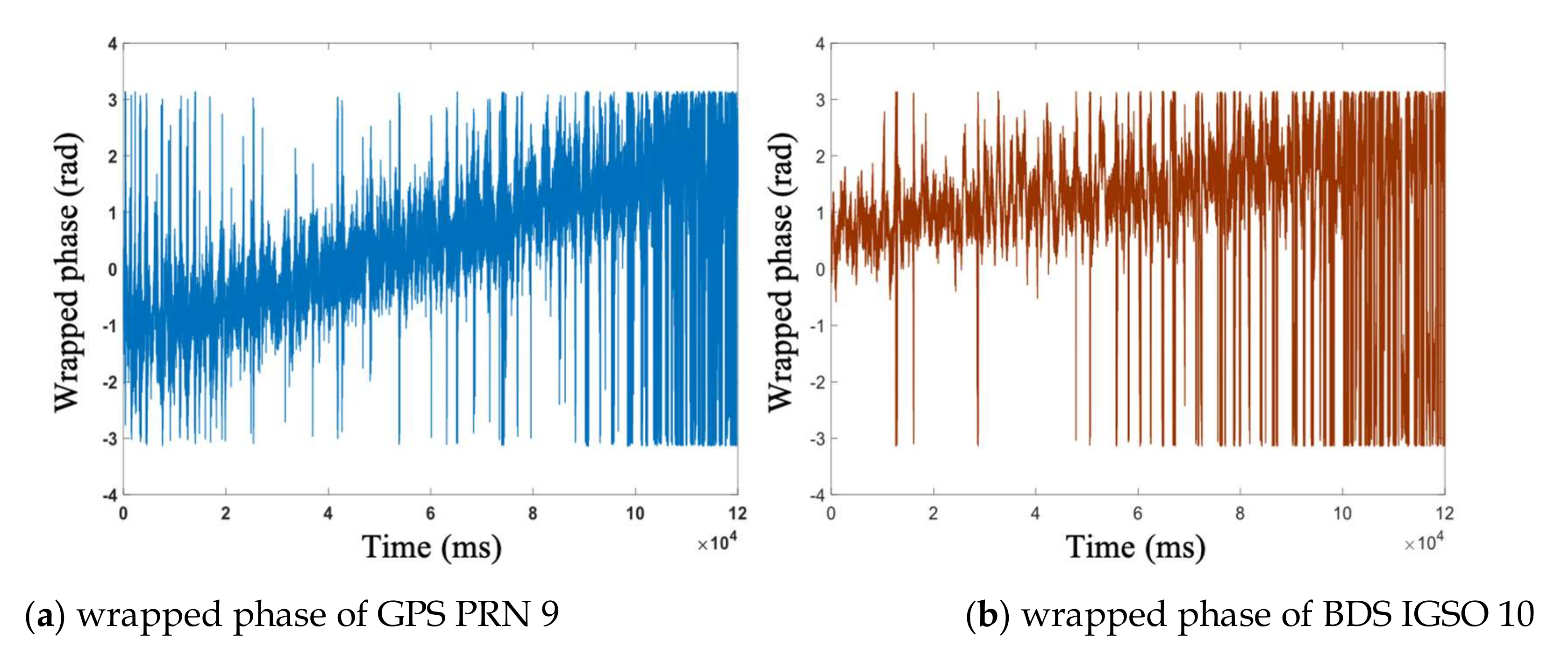
The raw residual phase ${\phi }_{out}$ is extracted from Equation (6) using the four-quadrant arctangent function. Figure 3a shows the wrapped phase of the GPS PRN 9 and Figure 3b shows the wrapped phase BDS IGSO 10 satellite in 2 min on 22 April 2021, 10:40 a.m.–10:42 a.m. (LT).

Figure 3. An example of wrapped phase of GPS PRN 9 (a) and BDS IGSO 10 (b) in 2 min (10:40 a.m.–10:42 a.m. local time).

The raw residual phase may exceed the phase interval [-π,$\mathsf{\pi }$], in which case the phase wrapping phenomenon occurs.

$${\phi }_{\mathit{residual}}=Unwarp[{\phi }_{\mathit{out}}]+2k\pi$$

(7)

where Unwarp [] represents the phase unwrapping operation, and ${\phi }_{residual}$ represents the result after the raw residual phase unwrapping, with k as the integer ambiguity.

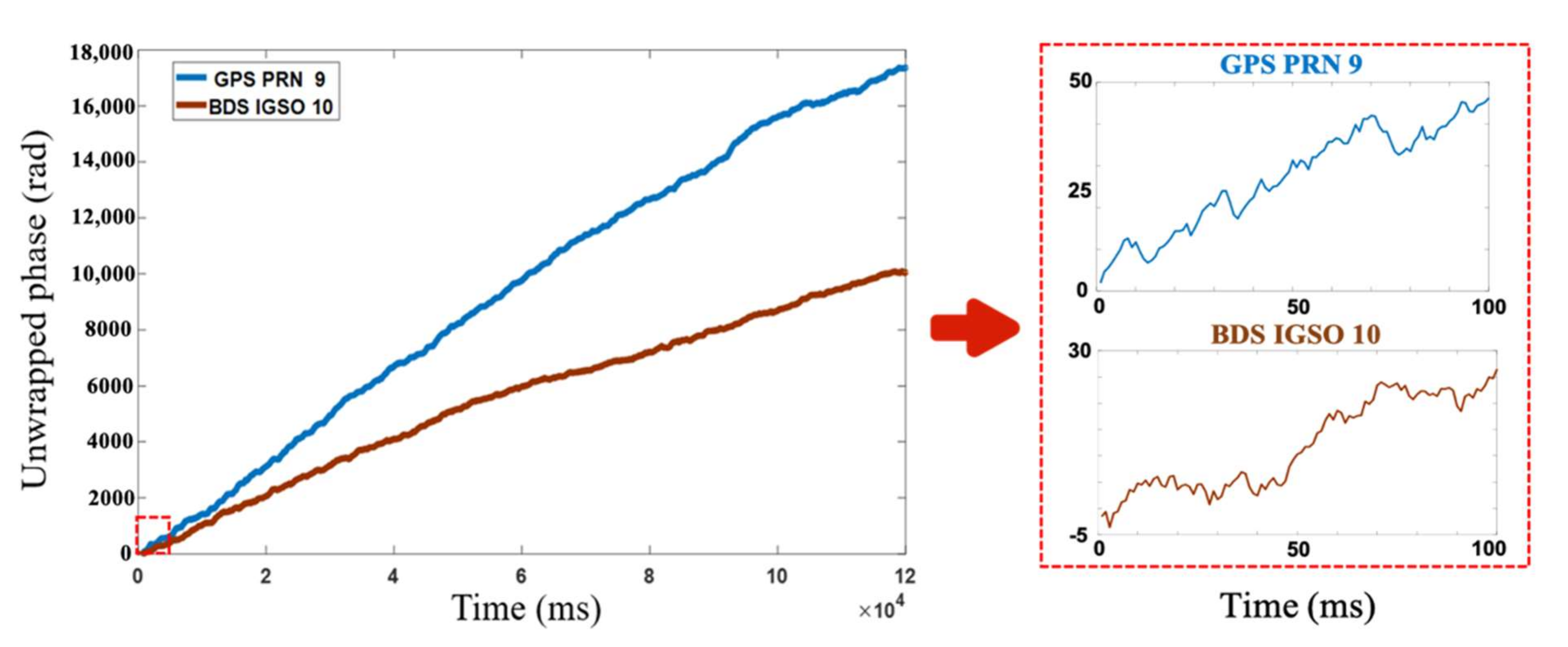
Figure 4 shows the residual phase after phase unwrapping of GPS PRN 9 and BDS IGSO 10 for 2 min on 22 April 2021, 10:40 a.m.–10:42 a.m. (LT). The first 100 ms unwrapped phase details are shown with red dashed boxes. The incoherence time in this paper is 1 ms, and the wrapped carrier phase in Figure 3 will be noisy in detail, but as long as the unwrapped carrier phase meets the relatively obvious linear trend, it can meet the requirements of inversion results every two min, as in this paper.

Figure 4. Unwrapped residual phase of GPS PRN 9 and BDS IGSO 10 in 2 min (10:40 a.m.–10:42 a.m. local time) (left panel); unwrapped phase details of GPS PRN 9 and BDS IGSO 10 in 100 ms (right panel).

2.3. Inversion Method

When GNSS satellite signals are reflected by the river in the target region, the Doppler frequency shift caused by the river flow velocity is the low-frequency component in the spectrum, due to the very low river flow compared with the satellite’s velocity. Moreover, the disconnected residual phase caused by random noise $N_i$ and $N_q$ only affects the high-frequency part of the frequency spectrum. In this article, GPS and BDS use the same inversion method.

By analyzing the residual phase spectrum of GNSS direct signal and reflected signal of the river to extract the low-frequency component of the spectrum, the inversion of river flow velocity can be realized. The geometric relationship of GNSS-R river flow inversion is shown in Figure 5.

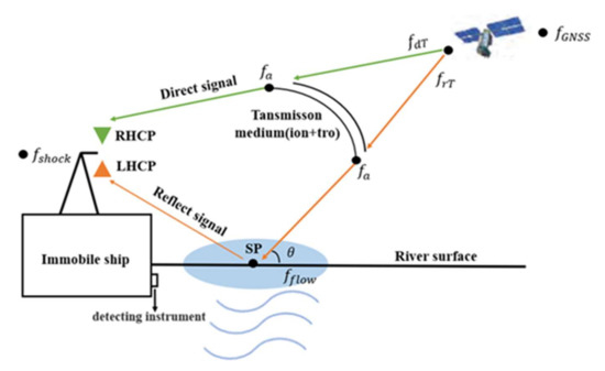
Figure 5. Geometric relationship of river flow velocity inversion.

In this paper, the principle of the reference [30] was expanded to apply to the inversion of river flow velocity under the experimental conditions of shore-based dual antennas. Unlike the experimental conditions of airborne experiments, under the conditions of shore-based experiments, there is no Doppler frequency caused by flight vibration. This paper explains in detail the magnitude and influence of each frequency component. The phase and frequency of the direct signal and reflected signal received by the receiver at time t are defined as follows:

$$\begin{array}{l}{\phi }_{\mathit{d}}(t)=2\pi {\mathit{f}}_{\mathit{d}}\cdot t\\ {\phi }_{\mathit{r}}(t)=2\pi {\mathit{f}}_{\mathit{r}}\cdot t\end{array}$$

(8)

$$\begin{array}{c}{\mathit{f}}_{\mathit{d}}={\mathit{f}}_{\mathit{GNSS}}-{\mathit{f}}_{\mathit{shock}}+{\mathit{f}}_{\mathit{dm}}+{\mathit{f}}_{\mathit{ds}}\\ {\mathit{f}}_{\mathit{r}}={\mathit{f}}_{\mathit{GNSS}}-{\mathit{f}}_{\mathit{shock}}+{\mathit{f}}_{\mathit{rm}}+{\mathit{f}}_{\mathit{ra}}+{\mathit{f}}_{\mathit{flow}}\end{array}$$

(9)

where $f_{GNSS}$ is the carrier frequency of satellite signals; the crystal vibration frequency of the receiver is $f_{shock}$ (the crystal vibration frequency of the GPS receiver used in this paper is 1575 MHz, and that of the BDS receiver is 1561 MHz); $f_{dm}\left(t\right)$ is the carrier Doppler frequency of direct signal due to satellite motion; $f_{rm}\left(t\right)$ is the carrier Doppler frequency of reflected signal carrier due to satellite movement; $f_{da}\left(t\right)$ and $f_{ra}\left(t\right)$ are the Doppler frequencies generated when the satellite signal propagates through the ionosphere and the atmosphere of the direct signal and reflected signal, respectively; the magnitude of $f_a\left(t\right)$ is near ${10}^{-2}$ Hz [35]. Since the receiver is fixed in the shore-based experiment, the receiver will not generate a Doppler frequency. Finally, $f_{flow}\left(t\right)$ refers to the Doppler frequency generated by the river.

Using the open-loop tracking method of Section 2.1, the residual interferometric phase ${\phi }_{out}$ of the unwrapped phase could be obtained:

$$\begin{array}{cc}\hfill {\phi }_{\mathit{out}}(t)& =2\pi ({\mathit{f}}_{\mathit{r}}-{\mathit{f}}_{\mathit{d}})\cdot t+\Delta \varphi \hfill \\ & =2\pi (\Delta {\mathit{f}}_{\mathit{m}}+\Delta {\mathit{f}}_{\mathit{a}}+{\mathit{f}}_{\mathit{flow}})\cdot t+\Delta \varphi \hfill \end{array}$$

(10)

where $\Delta f_m\left(t\right)=f_{rm}\left(t\right)-f_{dm}\left(t\right)$. Under shore-based experimental conditions, the delay of reflected signal and direct signal is within 1 ms. The path of direct/reflected signals are almost the same in the shore-based experiment set-up, so the satellite movement during the direct path and that during the reflected path are practically identical, and $\Delta f_m$ will be much lower than $f_{flow}\left(t\right)$.

Due to the shore-based experiment setup, the path of direct/reflected signals through the ionosphere and atmosphere is almost the same, $f_{da}\left(t\right)$ approximately equals $f_{ra}\left(t\right)$, and the value is simultaneously very small (${10}^{-2}$ Hz), so $\Delta f_a\left(t\right)=f_{ra}\left(t\right)-f_{da}\left(t\right)$ could also be ignored. Eventually, under shore-based experimental conditions, the parameters that have little influence on the inversion of river flow velocity are removed, and ${\phi }_{out}\left(t\right)$ can be written as follows:

$${\phi }_{\mathit{out}}(t)\approx 2\pi {\mathit{f}}_{\mathit{flow}}\cdot t+\Delta \varphi$$

(11)

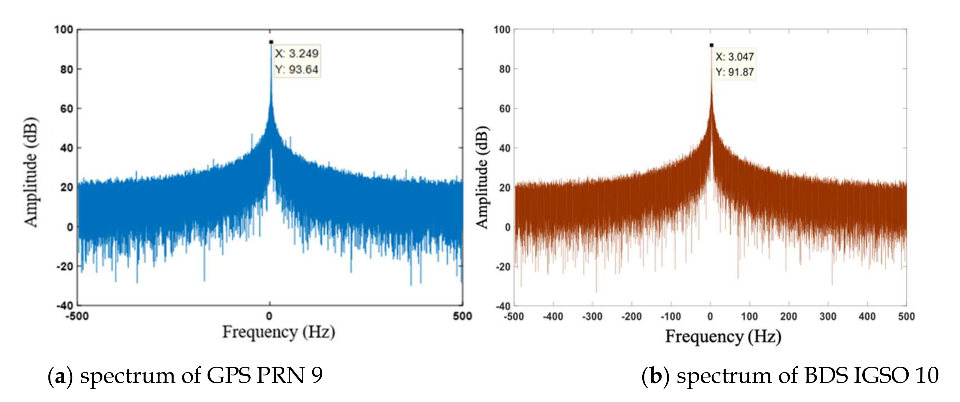
By FFT processing, the maximum value of the low-frequency component in the residual phase output spectrum $f_{flow}$ could be obtained from Equation (11). Figure 6 is the result of the FFT of the unwrapped residual phase (Figure 4) of the GPS PRN 9 and BDS IGSO 10 after unwrapping. Figure 6a is the spectrum of GPS PRN 9, the maximum value of the low-frequency component appears at 3.249 Hz and 3.047 Hz, which can be represented as the Doppler frequency $f_{flow}$ generated by river flow.

Figure 6. Spectrum analysis of GPS PRN 9 (a) and BDS IGSO PRN 10 (b) in 2 min (10:40 a.m.–10:42 a.m. local time).

Considering the geometric relations in Figure 5, the $V_{flow}$ could be deduced as follows [30]:

$${\mathit{V}}_{\mathit{flow}}={\mathit{f}}_{\mathit{flow}}\cdot \frac{c}{\cos (\theta )\cdot {\mathit{f}}_{\mathit{GNSS}}}$$

(12)

where $c$ is the light speed, $\theta$ is the elevation angle of satellite, $f_{flow}$ is the low-frequency Doppler component caused by river flow, and $f_{GNSS}$ is the carrier frequency of the satellite signal. According to the result of the maximum value of the low-frequency component in Figure 6 (upper panel 3.249 Hz and bottom panel 3.047 Hz), the flow velocity of the river can be calculated as 1.0217 m/s using GPS and 0.9758 m/s using BDS.

Considering a larger river flow velocity condition, in the case of $V_{flow}\approx$4 m/s and elevation $\theta \approx$50 degrees, $f_{flow}$ will be about 12 Hz according to Equation (12), which can be extracted from the residual phase using FFT. Therefore, this method can also be used under conditions of large river flow rates in theory, which is of great significance for water flow observation.

3. Shore-Based Velocity Inversion Experiment

3.1. The Experimental Set-Up

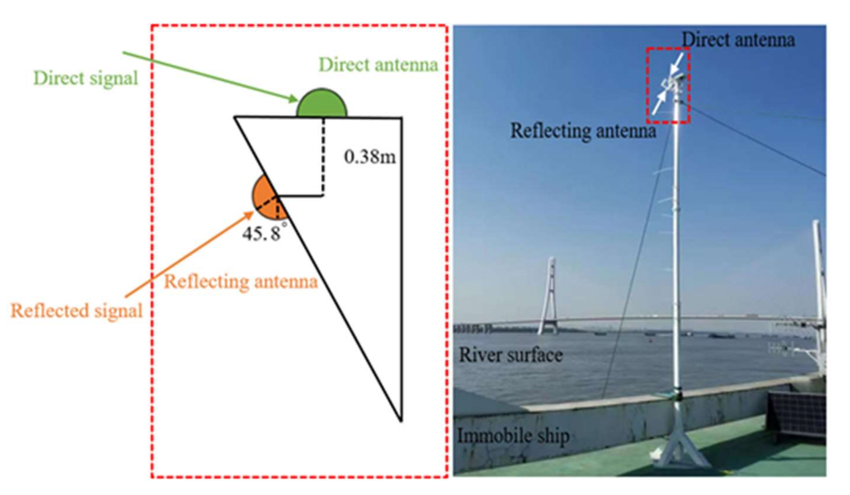
On 22 April 2021, a shore-based GNSS-R river flow velocity inversion experiment was carried out on the south bank of the Yangtze River basin (31°57′43″ N, 118°38′27″ E) near Dashengguan, Nanjing, China. The shore-based experiment was performed for almost 24 h, but because of damage to the receiver’s raw IF data reception during the experiment, the experimental results analysis only used about 2 h of data, from 9:30 a.m. to 11:30 a.m. (LT). Detection antennas and receiving equipment for receiving GPS/BDS dual-frequency direct/reflected signals were set up on the deck of a stationary cargo ship. The specific experimental set-up and antenna tilt settings are shown in Figure 7.

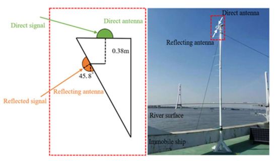
Figure 7. Experimental set-up.

The parameters were as follows: The direct antenna points upward to maximize direct signals’ contribution from above and to optimally suppress reflections. The height of the antenna is 5.45 m. The reflecting antenna points downwards with a tilt angle of 45.8 degrees, and the vertical height difference between the direct antenna and the reflecting antenna is 0.38 m. The orientation of the erected antenna is 304 degrees northwest (facing the Yangtze River). Table 1 is a summary of the experimental parameters.

Table 1. Experimental parameters.

Attributes	Value
Antenna latitude	31°57′43″ N
Antenna longitude	118°38′27″ E
Antenna azimuth angle	304° (northwest)
Tilt angle of reflecting antenna	45.8°
Height of antenna	5.45 m
Vertical height difference of direct/reflective antenna	0.38 m

3.2. Experimental Configuration

The hardware used in the experiment was a miniature GNSS-R detector designed and manufactured by Shanghai Aerospace Electronics Institute, which is made of a left-hand circular polarization antenna (LHCP), right-hand circular polarization antenna (RHCP), and hardware delay/Doppler-mapping receiver (DDMR). The device can receive GPS L1 and BDS B1I signals simultaneously.

A contact velocity-detecting instrument was used to record the average flow velocity from 9:30 a.m. to 11:30 a.m. (LT) every 5 min, which will be viewed as real velocity to assess inversion precision.

To meet the experimental requirements, the reflecting antenna of the receiver can receive the reflected signals in the area from negative 90 degrees to positive 90 degrees, and the reflecting antenna was set with a direction angle of 304 degrees northwest, so the azimuth of the region of the specular reflection point was chosen from 214 degrees to 34 degrees. Combining the zenith map with the screening scheme above, the experimental satellites selected in this paper are GPS PRN 4, PRN 9/BDS GEO 2, and IGSO 10. Figure 8 shows the zenith map of the selected experimental satellite at 10:00 a.m. (LT) on 22 April.

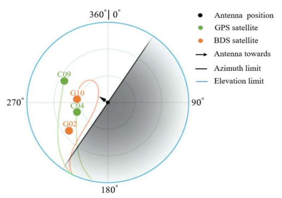
Figure 8. Satellite zenith at 10:00 a.m. (LT), 22 April 2021.

Figure 9 shows the movement track of the selected satellites’ specular points on 22 April. The red mark is the location of the erected antenna and the blue mark is the current meter location. The green circles are the starting points of GPS satellites’ specular points, and the orange circles are the starting points of BDS satellites’ specular points. Triangles represent the terminal of the corresponding specular reflection points. The white arrow represents the movement track of the satellite’s specular point. The white and red dashed lines delineate areas with the current meter at the center and a radius of 25 m and 50 m, respectively.

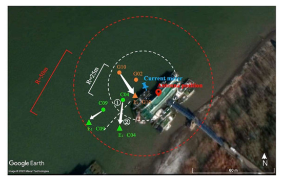
Figure 9. Movement trajectory of specular points. Circle points represent the beginning of specular points and triangle points represent the end of specular point. In this paper, the specular points in the red dotted line region are selected for inversion, and the “close points” in the white dotted line region are selected. In the figure, “①” represents the 1st period of GPS PRN4 inversion, and “②”represents the second stage of GPS PRN4 inversion.

As can be seen from Figure 9, since only one current meter is used in this experiment, there will be some difference between estimated river flow velocity on specular points and in situ measurements. We just chose the specular points within 50 m of the current meter (Figure 9, in the red dashed area) to reduce the difference impact in precision evaluation. Specular points within 25 m from the current meter are considered as the “close points” (Figure 9, in the white dotted area). Among specular points in Figure 9, PRN 4 specular points are divided into two periods due to environmental impact. In the 1st period, the specular points are almost “close points”; in the 2nd period, the specular points are obscured by platform obstacles.

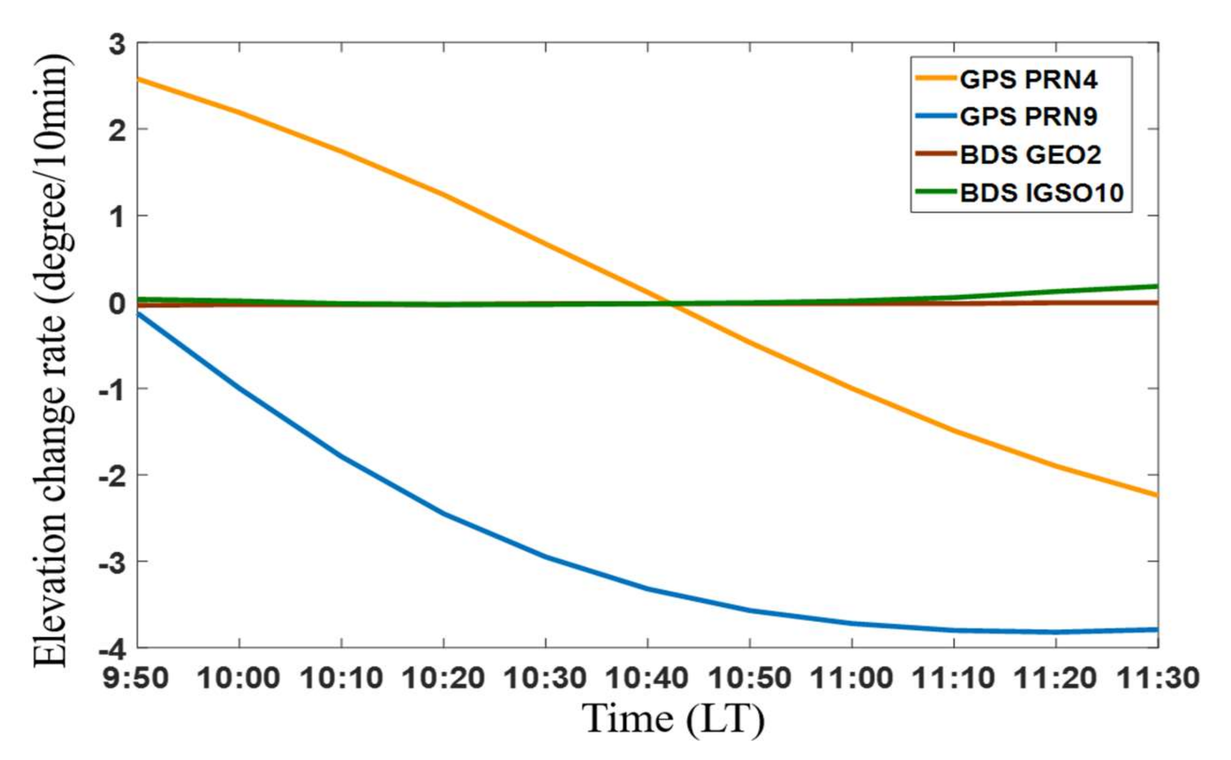
Figure 10 and Figure 11 record the elevation and elevation change rate of the selected satellites during the experimental period (GPS PRN 4, GPS PRN 9; BDS GEO 2, BDS IGSO 10).

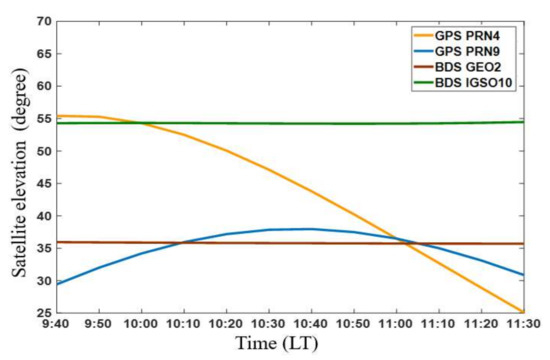
Figure 10. GNSS satellite elevation diagram.

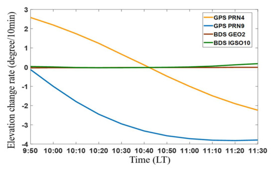
Figure 11. GNSS satellite elevation change rate diagram.

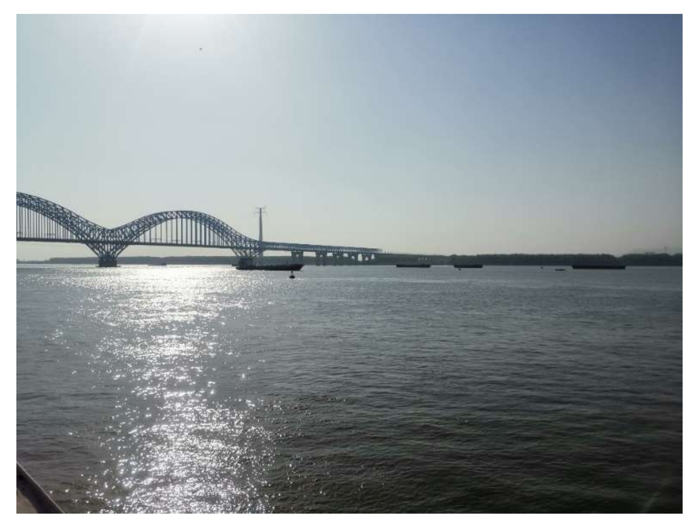
Surface water fluctuation is an important factor affecting the river’s surface roughness, and the wind speed affects the river’s surface roughness as well as the flow velocity of the river. Figure 12 shows a close-up view of the surface of the Yangtze River on the day of the experiment. During the experiment, the wind speed was small (not recorded), and the river surface was relatively stable. Therefore, we ignored the influence of river surface fluctuations on the monitoring of river flow velocity.

Figure 12. Photograph of the Yangtze River surface.

4. River Flow Velocity Inversion Result and Analysis

4.1. River Flow Velocity Inversion Results

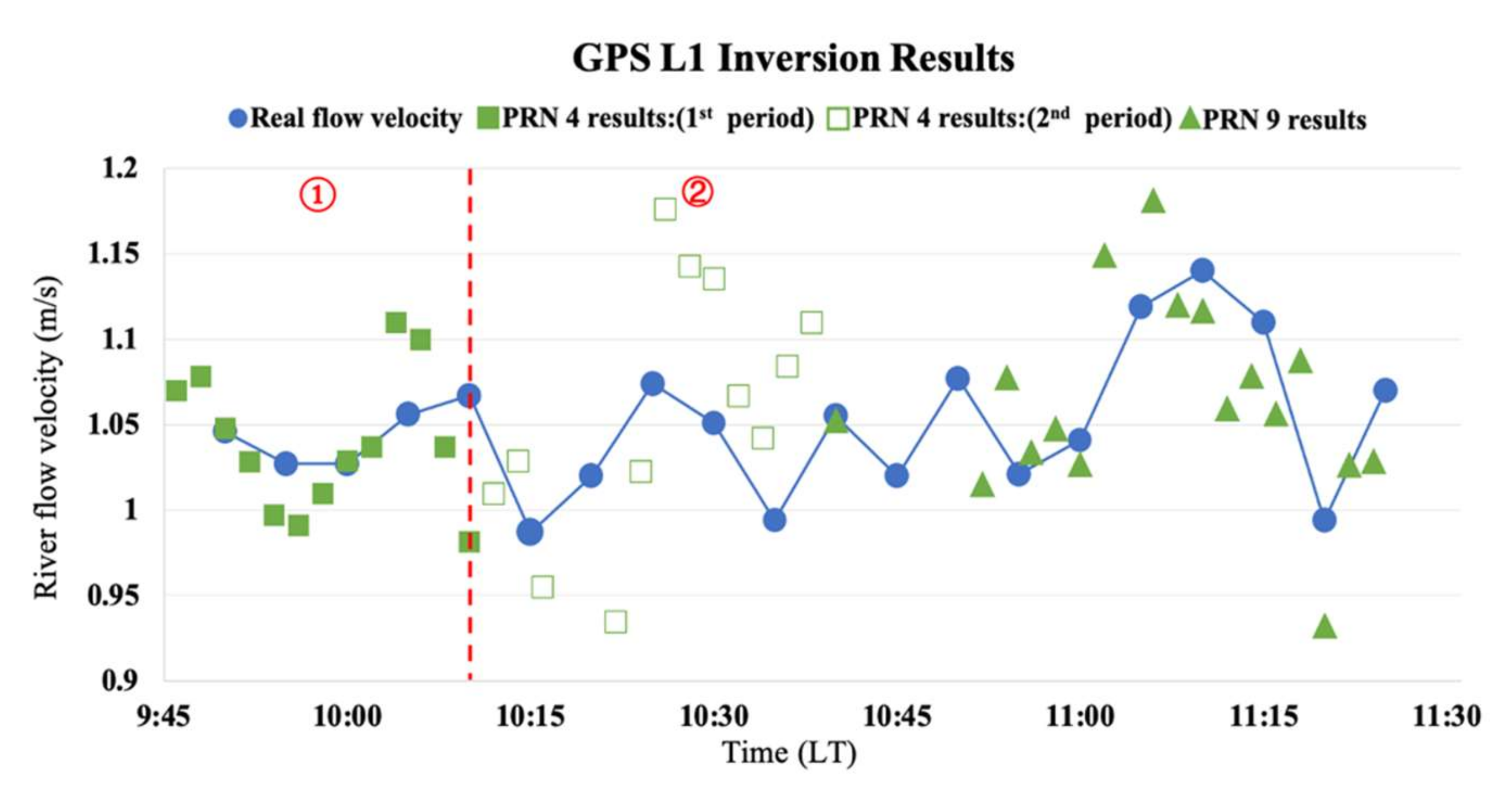
The inversion river flow velocity results per 2 min were calculated according to the shore-based carrier phase river flow velocity inversion method in Section 2. Figure 13 shows the GPS L1 inversion results. The blue solid circle represents the real river flow velocity $v_{real}$ per 5 min; green points are split up into squares (results of PRN 4) and triangles (results of PRN 9). Inversion results are shown in 2-min intervals. Figure 14 shows the BDS B1I inversion results. The blue solid circle represents the real river flow velocity $v_{real}$ per 5 min; orange points are split up into squares (results of GEO 2) and triangles (results of IGSO 10). Inversion results are shown in 2-min intervals.

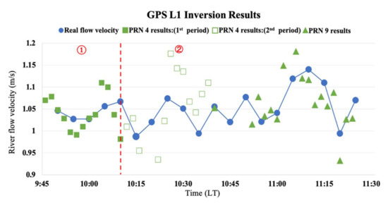
Figure 13. GPS L1 inversion results. In the figure, “①” represents the 1st period of GPS PRN4 inversion, and “②”represents the second stage of GPS PRN4 inversion.

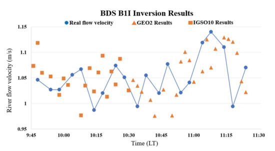
Figure 14. BDS B1I inversion results.

Four satellites’ (GPS PRN 4, GPS PRN 9, BDS GEO 2 and BDS IGSO 10) results and the accuracy verification results are listed in detail in Table 2.

Table 2. Accuracy of satellite inversion results.

Satellites System	PRN	Close Points Rate (Close Points/Total Points)	MAE(m/s)	RMSE(m/s)	R
GPS L1	PRN 4 (1st period)	100%	0.028	0.036	0.855
GPS L1	PRN 4 (2nd period)	13%	0.080	0.090	0.401
GPS L1	PRN 9	0%	0.103	0.14	0.378
BDS B1I	GEO 2	100%	0.048	0.063	0.806
BDS B1I	IGSO 10	100%	0.061	0.073	0.763

The Spearman correlation coefficient is used to measure relevance in this paper. The correlation coefficient R is as follows:

$$R=\frac{{\displaystyle {\sum }_i(xi-\overline{x})(yi-\overline{y})}}{\sqrt{{{\displaystyle {\sum }_i(xi-\overline{x})}}^2{\displaystyle {\sum }_i{(yi-\overline{y})}^2}}}$$

(13)

In the formula, $x_i$ and $y_i$ are correlated variables, $\overline{x}$ and $\overline{y}$ are the average values of the variables, and R ranges from −1 to 1. Generally, R > 0.7 demonstrates a strong correlation between variable, while 0.7 > R > 0.4 indicates there is a moderate correlation between variables.

By analyzing the results in Figure 13, Figure 14, and Table 2, GPS PRN 4 (1st period) inversion MAE reaches up to 0.028 m/s and root mean square error RMSE reaches 0.036 m/s. By contrast, GPS PRN 4 (2nd period) inversion MAE and RMSE are 0.080 and 0.090, respectively. The BDS IGSO 10 inversion MAE and RMSE are 0.061 m/s and 0.073 m/s, respectively. Compared with BDS IGSO 10 inversion results, the MAE and RMSE of BDS GEO 2 are improved by 0.013 m/s and 0.01 m/s, respectively, showing more accurate inversion results. R of PRN 4 (1st period), GEO 2, and IGSO 10 are higher than 0.7, showing strong correlation, which proves the effectiveness of inversion. Among these, a large gap existed between the inversion results of PRN 4 (1st period) and PRN 4 (2nd period). This may be due to the influence of obstacles or relatively fewer “close points”, as the current meter cannot accurately characterize the river velocity of specular points. The precision of PRN 9 is also lower than other inversion results, which may be due to the specular points of GPS PRN 9 being farther away from the current meter: the fixed current meter cannot represent the velocity at the specular points well, which affects the evaluation of results and the effectiveness of inversion.

4.2. Influence of Elevation Change Rate

It has been shown in Section 2.3 that the velocity of satellite movement has a direct influence on the elevation change rate of the satellite. Theoretically, the larger the elevation change rate is, the larger the $\Delta f_m\left(t\right)=f_{rm}\left(t\right)-f_{dm}\left(t\right)$ will be; $\Delta f_m\left(t\right)$ will superimpose with the low frequency $f_{flow}$ generated by the river flow and affect the inversion accuracy of river flow velocity. Figure 15 shows the sensitivity of river flow inversion accuracy to satellite elevation and elevation change rate, respectively.

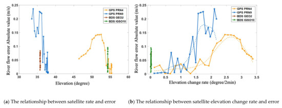
Figure 15. The relationship between satellite rate and error (a). The relationship between satellite elevation change rate and error (b).

The following can be concluded from the results: (1) satellite elevation (Figure 15a) has little influence on inversion accuracy; (2) on account of the low elevation change rate of the BDS satellite during the experimental period, the BDS satellite overall has the lowest elevation change rate and the more stable inversion precision (Figure 15b); and (3) the elevation change rate of satellites plays a significant role in the inversion precision of river flow velocity. The experimental inversion results are consistent with the theoretical hypothesis. It is worth mentioning that it can be seen in Figure 15 that over a relatively long period, the elevation angle change rate has a negative impact on the inversion accuracy. On the contrary, the GPS PRN 4 inversion results show an abnormal phenomenon for a short time when the elevation angle change rate is greater than 2.5 degree/min. This may be due to the velocity recorded by the current meter being incidentally close to that at the specular reflection point of THE GPS PRN 4; because of this, a deviation exists between the water flow velocity at the specular point and the water flow velocity detected by the river current meter.

Table 3 shows the correlation coefficient between inversion accuracy and elevation change rate. R of GPS 4 and GPS 9 are 0.652 and 0.876, respectively. The comprehensive correlation coefficient reaches up to 0.727, proving a strong correlation between the inversion accuracy error and the elevation angle change rate.

Table 3. Correlation analysis between precision and elevation change rate.

Satellite System	PRN	R
GPS L1	PRN 4	0.652
GPS L1	PRN 9	0.876
GPS L1	ALL	0.727

4.3. Influence of Reflected Signal Strength

The quality and strength of the signal can be measured by the signal-to-noise ratio (SNR) of the reflected signal. In this paper, I and Q of the reflected signal are used to calculate the SNR. Figure 16 shows the Lissajous figures of four satellites (GPS PRN 4, PRN 9, BDS GEO 2, and IGSO 10) to display the I and Q branches of the reflected signal demodulated by the software receiver.

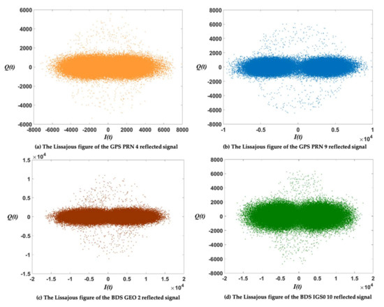
Figure 16. The Lissajous figures of four satellites’ reflected signals. The Lissajous examples include GPS PRN 4 SNR 10:00–10:02 a.m. (LT), GPS PRN 9 SNR 11:00−11:02 a.m. (LT), BDS GEO 2 SNR 10:00–10:02 a.m. (LT), and BDS IGSO 10 SNR 11:00−11:02 a.m. (LT).

The carrier-to-noise ratio (CNR) of a reflected signal can be defined as follows [31]:

$$CNR=10lg(\frac{({\mathit{I}}_{\mathit{i}}^2+{\mathit{Q}}_{\mathit{i}}^2)}{{(\sqrt{{\mathit{I}}_{\mathit{i}}^2+{\mathit{Q}}_{\mathit{i}}^2}-\frac{1}{N}{\displaystyle \sum _{i=1}^N\sqrt{{\mathit{I}}_{\mathit{i}}^2+{\mathit{Q}}_{\mathit{i}}^2}})}^2})$$

(14)

where N is the signal tracking time (2 min). The unit of SNR is decibel (dB). After completing the signal carrier synchronization and baseband demodulation processing, SNR and CNR have the following relationship:

$$SNR={\mathit{G}}_{\mathit{B}}+CNR$$

(15)

where G_B is baseband signal gain, including coherent cumulative gain value G_C, incoherent cumulative gain value G_I, and square loss G_L:

$${\mathit{G}}_{\mathit{B}}={\mathit{G}}_{\mathit{C}}+{\mathit{G}}_{\mathit{I}}-{\mathit{G}}_{\mathit{L}}$$

(16)

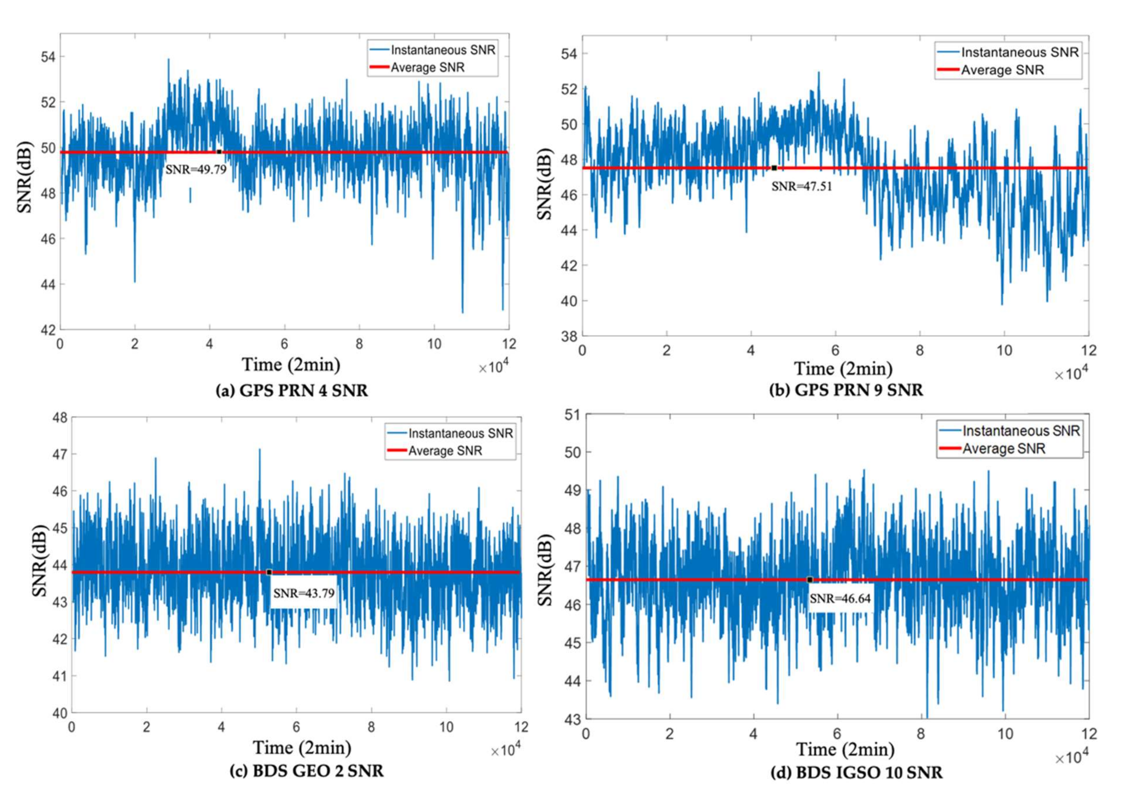
SNR is obtained by demodulating the I and Q branch of the raw IF data by the software receiver [36], including the instantaneous SNR and the average SNR in Figure 17. The instantaneous SNR fluctuates over time, so the average SNR is selected as the standard for evaluating signal strength. The SNR of GPS PRN 4, GPS PRN 9, BDS GEO 2, and BDSI GSO 10 in this period are 49.76 dB, 47.51 dB, 43.79 dB, and 46.64 dB, respectively. MEO signal strength of GPS is slightly stronger than the signal strength of GEO and IGSO of BDS. The four satellites analyzed in this experiment all have good signal quality. The influence of signal quality on the inversion accuracy cannot be judged by the slight difference between the average SNR of the four satellites. Combining the analysis of the results in Table 2, there is no apparent correlation between signal strength and the inversion accuracy of shore-based river flow velocity.

Figure 17. SNR of four satellites’ reflected signals (GPS PRN 4 (a), PRN 9 (b), BDS GEO 2 (c), and IGSO 10 (d)). Blue represents the instantaneous SNR, and red represents the average SNR in 2 min.

5. Conclusions

In this paper, the GNSS-R river current measurement was carried out on the south bank of Dashengguan Yangtze River in Nanjing, China, for nearly two h on 22 April 2021. The self-developed GNSS-R soft receiver was used to process satellites’ direct and reflected signals. The Doppler frequency is extracted by the interferometric carrier phase of the direct signal, and the reflected signal is proposed for inverse river flow velocity. The accuracy of the inversion results is verified by using the actual obtained data. This shore-based experiment realized the detection of river flow velocity and achieved high accuracy. More importantly, the possibility of BDS-R inversion of river flow velocity was verified for the first time.

This article qualitatively analyzes the inversion results from three perspectives: (1) relative position of specular points to current meter, (2) elevation angle, (3) elevation angle change rate, and (4) signal strength. The following conclusions can be drawn from the inversion results of this experiment:

In the case that the specular points are far away from the current meter or the specular points are blocked by obstacles, the current meter may not accurately represent the flow velocity, which leads to a large error between the flow velocity results of experimental inversion and the flow velocity results recorded by the current meter, which affects the evaluation of results and the effectiveness of inversion.

The MAE and RMSE of GPS PRN 4 (1st period) inversion results are 0.028 m/s and 0.036 m/s, respectively. The MAE and RMSE of BDS GEO 2 and IGSO 10 inversion results are 0.049 m/s and 0.063 m/s, and 0.061 m/s and 0.073, respectively. Both achieve high inversion accuracy, which proves the effectiveness of the inversion model of river flow velocity.

The analysis of elevation results and the SNR of different satellites show that signal strength and elevation of satellites have obvious correlations with the inversion accuracy of river flow velocity in this shored-based experiment.

Because the elevation angle of specular points of the BDS GEO 2 and IGSO 10 satellites is little changed during the period of the experiment, the Doppler frequency value generated by satellite motion is very small, while the elevation change rate of the GPS MEO satellite is larger, and the Doppler frequency generated by satellite motion is larger than the former. The inversion results show that the inversion results of BDS GEO 2 and IGSO 10 are superior to those of GPS PRN 4 and GPS PRN 9. The elevation angle change rate of GEO 2 is almost close to 0 degrees/minute. Its achieved inversion precision was the best. The decrease of elevation change rate directly reduces the Doppler frequency shift difference $\Delta f_T$ between direct and reflected signals and is more conducive to inversion of river flow velocity.

Apart from the factors discussed in this article, whether the differences between GPS and BDS systems in other aspects would impact the inversion accuracy of river flow velocity should be explored in future studies. Longer-term experimental data (more than 24 h), more river current meters, and more environmental data (such as wind speed, etc.) should be used in the future to verify the factors affecting river flow rate under different conditions.

References

- Sauquet, E.; Shanafield, M.; Hammond, J.C.; Sefton, C.; Datry, T. Classification and trends in intermittent river flow regimes in Australia, northwestern Europe and USA: A global perspective. J. Hydrol. 2021, 597, 126–170. [Google Scholar] [CrossRef]
- Sanjou, M.; Shigeta, A.; Kato, K.; Aizawa, W. Portable unmanned surface vehicle that automatically measures flow velocity and direction in rivers. Flow Measurement and Instrumentation. Flow Meas Instrum. 2021, 6, 2411–2502. [Google Scholar] [CrossRef]
- Wang, H.; Zang, J.; Wang, X. Research and Application of the Flow Calculation Model Based on the Average Velocity Distribution of the Vertical Line of the Cross Section. Hydrology 2019, 49, 50–54. [Google Scholar]
- Zhang, Y.; Xie, X.; Meng, W. Bohai Sea Ice Detection Based on Beidou GEO Satellite Reflected Signal. J. Beijing Univ. Aeronaut. Astronaut. 2018, 44, 257–263. [Google Scholar] [CrossRef]
- Zhang, Y.; Ma, D.; Meng, W. Research on sea level inversion of GPS Reflection Signal based on Techdemosat-1 satellite. J. Beijing Univ. Aeronaut. Astronaut. 2019, 10, 1941–1948. [Google Scholar] [CrossRef]
- Zhang, Y.; Hang, S.; Han, Y. Sea Ice Thickness Detection Using Coastal BeiDou Reflection Setup in Bohai Bay. IEEE Geosci. Remote. Sens. Lett. 2020, 99, 1–5. [Google Scholar] [CrossRef]
- Rodriguez-Alvarez, N.; Akos, D.M.; Zavorotny, V.U. Airborne GNSS-R Wind Retrievals Using Delay–Doppler Maps. IEEE Trans. Geosci. Remote Sens. 2013, 51, 626–641. [Google Scholar] [CrossRef]
- Valencia, E.; Zavorotny, V.U.; Akos, D.M. Using DDM Asymmetry Metrics for Wind Direction Retrieval From GPS Ocean-Scattered Signals in Airborne Experiments. IEEE Trans. Geosci. Remote Sens. 2014, 52, 3924–3936. [Google Scholar] [CrossRef]
- Zavorotny, V.U.; Voronovich, A.G. Scattering of GPS signals from the ocean with wind remote sensing application. IEEE Trans. Geosci. Remote Sens. 2000, 38, 951–964. [Google Scholar] [CrossRef] [Green Version]
- Yan, Q.; Huamg, W. Spaceborne GNSS-R Sea Ice Detection Using Delay-Doppler Maps: First Results From the U.K. TechDemoSat-1 Mission. IEEE J.-STARS. 2016, 9, 4795–4801. [Google Scholar] [CrossRef]
- Alonso-Arroyo, A.; Zavorotny, V.U.; Camps, A. Sea Ice Detection Using U.K. TDS-1 GNSS-R Data. IEEE Trans. Geosci. Remote Sens. 2017, 55, 4989–5001. [Google Scholar] [CrossRef] [Green Version]
- Zhu, Y.; Tao, T.; Zou, J. Spaceborne GNSS reflectometry for retrieving sea ice concentration using TDS-1 data. IEEE Trans. Geosci. Remote Sens. 2020, 18, 612–616. [Google Scholar] [CrossRef]
- Gerlein-Safdi, C.; Ruf, C.S. A CYGNSS-based algorithm for the detection of inland waterbodies. Geophys. Res. Lett. 2019, 46, 12065–12072. [Google Scholar] [CrossRef]
- Ghasemigoudarzi, P.; Huang, W.; Silva, O.D. A machine learning method for inland water detection using CYGNSS data. IEEE Geosci. Remote. Sens. Lett. 2020, 19, 8001105. [Google Scholar] [CrossRef]
- Valencia, E.; Camps, A.; Rodriguez-Alvarez, N. Using GNSS-R Imaging of the Ocean Surface for Oil Slick Detection. IEEE J.-STARS 2013, 6, 217–223. [Google Scholar] [CrossRef]
- Li, C.; Huang, W.; Gleason, S. Dual Antenna Space-Based GNSS-R Ocean Surface Mapping: Oil Slick and Tropical Cyclone Sensing. IEEE J.-STARS 2015, 8, 425–435. [Google Scholar] [CrossRef]
- Ca Parrini, M.; Egido, A.; Soulat, F. Oceanpal: Monitoring sea state with a GNSS-R coastal instrument. In Proceedings of the 2007 IEEE International Geoscience and Remote Sensing Symposium, Barcelona, Spain, 23–28 July 2007; pp. 23–28. [Google Scholar]
- Larson, K.M.; Ray, R.D.; Nievinski, F.G. The Accidental Tide Gauge: A GPS Reflection Case Study From Kachemak Bay. IEEE Trans. Geosci. Remote Sens. Lett. 2013, 10, 1200–1204. [Google Scholar] [CrossRef] [Green Version]
- Treuhaft, N.; Lowe, S.T.; Zuffada, C. 2-cm GPS altimetry over Crater Lake. Geophys. Res. Lett. 2001, 28, 4343–4346. [Google Scholar] [CrossRef]
- Mashburn, J.; Axelrad, P.; Lowe, S.T. An Assessment of the Precision and Accuracy of Altimetry Retrievals for a Monterey Bay GNSS-R Experiment. IEEE J.-STARS 2017, 9, 4660–4668. [Google Scholar] [CrossRef]
- Zhang, Y.; Li, B. Phase Altimetry Using Reflected Signals From BeiDou GEO Satellites. IEEE Trans. Geosci. Remote Sens. 2016, 13, 1–5. [Google Scholar] [CrossRef]
- Cardellach, E.; Rius, A.; Martín-Neira, M. Consolidating the precision of interferometric GNSS-R ocean altimetry using airborne experimental data. IEEE Trans. Geosci. Remote Sens. 2013, 52, 4992–5004. [Google Scholar] [CrossRef]
- Carreno-Luengo, H.; Park, H.; Camps, A. GNSS-R Derived Centimetric Sea Topography: An Airborne Experiment Demonstration. IEEE IGARSS 2013, 6, 1468–1478. [Google Scholar] [CrossRef]
- Fabra, F.; Cardellach, E.; Ribo, S. Is Accurate Synoptic Altimetry Achievable by Means of Interferometric GNSS-R? Remote Sens. 2019, 11, 505–520. [Google Scholar] [CrossRef] [Green Version]
- Hu, C.; Benson, C.; Rizos, C. Single-Pass Sub-Meter Space-Based GNSS-R Ice Altimetry: Results From TDS-1. IEEE J.-STARS 2017, 11, 3782–3788. [Google Scholar] [CrossRef]
- Li, W.; Cardellach, E.; Fabra, F. First spaceborne phase altimetry over sea ice using TechDemoSat-1 GNSS-R signals. Geophys. Res. Lett. 2017, 44, 8369–8376. [Google Scholar] [CrossRef]
- Li, W.; Cardellach, E.; Fabra, F. Lake Level and Surface Topography Measured with Spaceborne GNSS in eflectometry from CYGNSS Mission: Example for the Lake Qinghai. Geophys. Res. Lett. 2018, 45, 313–332. [Google Scholar] [CrossRef]
- Zuffada, C.; Haines, B.; Hajj, G. Assessing the Altimetric Measurement from CYGNSS Data. In Proceedings of the IGARSS 2018—2018 IEEE International Geoscience and Remote Sensing Symposium, Valencia, Spain, 22–27 July 2018; Volume 7. [Google Scholar]
- Semmling, A.M.; Schmidt, T.; Wickert, J.; Schön, S.S.; Fabra, F.; Cardellach, E.; Rius, A. On the retrieval of the specular reflection in GNSS carrier observations for ocean altimetry. Radio Sci. 2012, 47, RS6007. [Google Scholar] [CrossRef]
- Bai, W.; Xia, J.; Wei. W. A first comprehensive evaluation of China’s GNSS-R airborne campaign: Part II-river remote sensing. Sci. Bull. 2015, 17, 1527–1534. [Google Scholar] [CrossRef] [Green Version]
- Lu, Y. Principle and Implementation Technology of Beidou/GPS Dual-Mode Software Receiver, 3rd ed.; Publishing House of Electronics Industry: Beijing, China, 2016; pp. 163, 204–206, 212. [Google Scholar]
- Lu, Y. GPS Global Positioning Receiver: Principle and Software Implementation, 1st ed.; Publishing House of Electronics Industry: Beijing, China, 2009; pp. 76–78. [Google Scholar]
- Yang, D. Zhang, Q. GNSS Reflected Signal Processing Basis and Practice: GNSS Reflected Signal Processing Basis and Practice, 1st ed.; Publishing House of Electronics Industry: Beijing, China, 2012; pp. 76–77, 90–91. [Google Scholar]
- Beyerle, G.; Schmidt, T.; Wickert, J. Observations and simulations of receiver-induced refractivity biases in GPS radio occultation. J. Geophys. Res. 1970, 111, D12. [Google Scholar] [CrossRef] [Green Version]
- Geng, Q.; Huang, Z.; Li, Q. Doppler shift estimation and compensation of low and medium orbit satellite signals. Systems Eng. Electron. 2009, 31, 256–260. [Google Scholar] [CrossRef]
- Wang, J.W. Signal-to-Noise Ratio (SNR). Encycl. Neurosci. 2008, 47, 4833–4840. [Google Scholar] [CrossRef]
Publisher’s Note: MDPI stays neutral with regard to jurisdictional claims in published maps and institutional affiliations. |
© 2022 by the authors. Licensee MDPI, Basel, Switzerland. This article is an open access article distributed under the terms and conditions of the Creative Commons Attribution (CC BY) license (https://creativecommons.org/licenses/by/4.0/).