On Spectral-Spatial Classification of Hyperspectral Images Using Image Denoising and Enhancement Techniques, Wavelet Transforms and Controlled Data Set Partitioning

Abstract

Obtaining relevant classification results for hyperspectral images depends on the quality of the data and the proposed selection of the samples and descriptors for the training and testing phases. We propose a hyperspectral image classification machine learning framework based on image processing techniques for denoising and enhancement and a parallel approach for the feature extraction step. This parallel approach is designed to extract the features by employing the wavelet transform in the spectral domain, and by using Local Binary Patterns to capture the texture-like information linked to the geometry of the scene in the spatial domain. The spectral and spatial features are concatenated for a Support Vector Machine-based supervised classifier. For the experimental validation, we propose a controlled sampling approach that ensures the independence of the selected samples for the training data set, respectively the testing data set, offering unbiased performance results. We argue that a random selection applied on the hyperspectral dataset to separate the samples for the learning and testing phases can cause overlapping between the two datasets, leading to biased classification results. The proposed approach, with the controlled sampling strategy, tested on three public datasets, Indian Pines, Salinas and Pavia University, provides good performance results.

1. Introduction

Our environment is composed of different materials, which may seem similar to the human eye in visible white light, but which have other characteristics in monochromatic, infrared, or ultraviolet light [1]. Some of these features, which are not visible to the naked human eye, are integrated into the field of hyperspectral imaging and spectroscopy [2]. The hyperspectral image (HSI) takes the response of a surface/material under electromagnetic radiation at different wavelengths, both inside and outside the visible spectrum to obtain a characteristic spectral representation of it [2,3].

The importance and relevance of hyperspectral imaging is given by its ability to discriminate between different materials based on the patterns exhibited in the spectral domain/resolution of the data, but also by its ability to analyze a small spatial structure or pattern in the spatial domain [4]. By combining rich spectral information with spatial information, hyperspectral images can achieve increasingly accurate classifications of great importance in agriculture [5], forestry [6] and other fields [7,8]. For example, the classification of the hyperspectral image has become a dynamic and interesting field of research. Making a comparison between the representation of traditional RGB images and hyperspectral images, the latter look more like 3D data cubes; therefore, it is necessary to explore the various classification methods properly designed and optimized for this special type of data structures [9].

In the three-dimensional representation of the hyperspectral images (HSI), the first two dimensions represent the information stored in space (the 2D geometry of the object, like any monochromatic/black and white image), having M rows, N columns; the third dimension represents the spectral information of different scene objects spread across B spectral bands. This manner used for data representation is illustrated in Figure 1. The HSIs, of size M × N × B, like any captured data, are noisy, so assuming an additive noise model, the observed HSI image, denoted as F is:

F = U + n,

(1)

with U being the noise-free data and n the noise. As described in [10], the noise in HSI images has different intensities along the spectral bands.

Most hyperspectral datasets are obtained from setups that collect a continuous representation of the data along the spectrum (wavelength of light). This translates into large amounts of information capable of providing a great deal of detail, but with the downfall of having an increase in processing time during analysis. By reducing the problem to a discrete number B of spectrally narrow bands, representations like those in Figure 1 can be obtained.

For a similarly looking object or material, in terms of geometrical patterns, HSI provides cues for developing algorithms that can cope with the variability in the spectral domain of the data and provide a relevant classification of objects and materials in the scene for a better scene understanding. Each individual pixel is characterized by the spectral signature for a certain type of material. Depending on the relationship between different details in the spatial domain and those related to the scene (e.g., number of pixels for a certain scene or object of similar material) some relevant information that can be used for classification is given by the strong correlations between adjacent pixels. Those relations foster the need for classification methods designed specifically for these types of images [11], where spatial and spectral data are considered jointly and where it is possible to encounter the phenomenon of the same object with different spectra and different objects with the same spectrum [12]. These phenomena, on the other hand, restrict the accuracy of classification, as the dimensionality of the problem increases and the size of the training set may not be sufficient to extract all relevant parameters, causing overfitting of the classifier (the Hughes phenomenon [13]). However, as spatial resolution increases, the HSI image provides richer spatial structures and texture features, increasing the available data and data variability along the spatial dimension as well, which helps to increase the accuracy of the classification [14]. This also mitigates the problem of the low/medium spatial resolution of HSI data for Earth observation, where, if pixels cover large spatial regions, there is a tendency to generate mixed spectral signatures, leading in turn to high interclass similarity in border regions [15].

State-of-the-art classification techniques have been developed successfully for some HSI applications [16]. However, the methods thus developed tend to face difficulties in realistic situations, where the selection of labeled training samples available in the HSI classification is usually small [17], which leads to the problem of classifying images based on small sample sizes.

More than the problem of the insufficient labeled available datasets, hyperspectral images may also present artifacts resulting from uncontrolled changes in the reflectance captured by the spectrometer (the presence of clouds/changes in the atmospheric conditions, etc.) or instrumental noise corrupting spectral bands data [18].

To cope with the large amount of information stored in hyperspectral images, but also to avoid the problem imposed by such large sizes of the data, two main families of approaches are mentioned in the literature [19] focusing on methods for feature extraction and, secondly, focusing on methods for feature selection. Methods for extracting new features allow the creation of new descriptors from the original bands, whereas the feature selection methods must allow the extraction from the data cube of the most relevant information stored in the spectral bands. The two approaches will be combined in this paper in the proposed processing framework.

In a previous work, [20], we investigated how hyperspectral images can be filtered and enhanced so as not to destroy any of the relevant information existing in either the spatial (geometry of the scene) dimension or the spectral one. In our study from [21], we focused on feature descriptors for the complex HSI data and opened the case for approaching this component in the processing pipeline, again considering the coupling of the two dimensions of the data. In this work, we focused on proposing an end-to-end approach for HSI data processing, consisting of filtering and enhancing stages, followed by a feature extraction step and a classification phase. All stages consider the simultaneous processing of the spatial and spectral information in the data. With this respect, we investigated how the choice of partitioning the available HSI datasets into a training subset and a testing subset when supervised learning classifiers are used can bias the results and provide misleading classification results. Thus, in the proposed work we also include a method for controlled data sampling, ensuring proper independence between the two subsets and, subsequently, trustworthy labeling results.

We refer to our processing sequence as being an end-to-end parallel one by referring to the classification in [22] where the difference between the integrative and the parallel is given. More, by including a denoising step, data does not require any pre-processing.

The rest of the paper is organized as follows. Section 2 describes the related work. The overall addressed challenges by this work and the proposed methods used are explained in detail in Section 3. In Section 4 we detail the chosen datasets and their proposed partitioning method, the experimental setup configuration and provide the results obtained both in terms of accuracy in classification and visual results. The discussions are reserved for Section 5 and the conclusions are given in Section 6.

2. Related Work

Spectral images, like any type of image, are affected by noise, [18], limiting the quality of the desired classification results. To reduce the noise in a hyperspectral image, different approaches have been advocated. Krishnamurthy, in [23], partitioned a hyperspectral cube into anisotropic cells and maximized a penalized log-likelihood criterion. Furthermore, variational approaches have been applied on HSI, such as the total variation (TV), proving to be effective and capable of preserving the edges in the data. In [24], a spectral-spatial adaptive model based on the seminal work of Rudin–Osher–Fatemi (ROF) from [25] was employed, showing relevant classification results, even when the noise level is different in each band. In [26], the authors proposed a hybrid spatial-spectral derivative-domain wavelet shrinkage that benefits from the dissimilarity of the signal regularity in the spatial and spectral dimensions of the HSI. The algorithm allows a degree of smoothness that can be adjusted, but the spatial-spectral dependencies of HSI images are not considered. Being a pseudo-3D data cube, the hyperspectral image is represented not only in the spectral dimension but also in the spatial one. To consider those dependencies, the combined spatial and spectral weighted hyperspectral total variation (CSSWHTV) model is introduced in the work of Yuan [27], combining the total spectral and spatial weighted hyperspectral variation.

Initially, the HSI classification was based only on information provided by the spectral dimension, but those spectral features are not enough to represent and distinguish the different objects or elements present in a hyperspectral image (HSI). In [28], a multi-scale feature extraction classification framework is introduced, capable of improving the accuracy of HSI classification due to the decomposition of the HSI into multi-scale structures through a Gaussian pyramid model, with the advantage of preserving detailed structures at the edge regions of the image.

Based on the same concept of dependency between the two dimensions, spatial and spectral, a spectral-spatial method for classification of hyperspectral images is presented in [29], where an edge weighting function, based on low-frequency edge weighting is designed for the spatial dimension, while a combined spectral and spatial Laplacian matrix is used in classification.

Both [28] and [29] approaches take into consideration the HSI classification problem by having an altered representation of the HSI data cube, incorporating a stage dedicated to feature extraction followed by a stage for feature classification. Recent advances in deep learning methods challenge this approach, by providing processing architectures that no longer require handcrafting feature extraction methods, but rather rely on the training step to extract information that structures the weights of a neural network. We refer the reader to the work of Paoletti, in [7], for an extensive overview of the field, including discussions regarding available datasets and dataset partitioning for training and testing limiting the benefits of such approaches. Even in [17], it is argued that there is an extensive gap between the benefits of deep learning methods and practical situations where the lack of labeled data for training causes these deep learning methods to require further investigation and research. In [17], the author does not consider, however, the unbiased partitioning of the dataset between the training and testing phase of the experiments.

Feature extraction is the method that takes the input data, transforms and translates it into another space of representation—one that contains most of the relevant information—and is considered pertinent for the classification task [30]. The texture of an image can be defined as a set of values used to quantify the perceived texture of an image. Regarding the way the parameters describing the texture in an image are represented, one can mention the frequency domain representation, the entropy of the image, the homogeneity, the local binary pattern (LBP), etc.

A relevant use case for texture characterization and feature extraction is the reduction of the dimensionality of the data, without losing valuable information from the original data set [31]. Methods like the principal component analysis (PCA) [32], and the canonical analysis (CA) [33], aim at this by transforming the hyperspectral pixel vectors into a new set of coordinates.

Hyperspectral data is classified using different approaches such as k-closest-neighbors [33], maximum probability criterion [34], support vector machine, and logistic regression [35]. The accuracy of the classification of these methods is mostly unsatisfactory, due to the insufficient number of training samples compared to a large number of spectral bands [13]. With respect to this, random sampling of the data set to first train the model and then to validate (test) it, generate distributions in the data that bias the classification results: almost the same data is present in both subsets, so any new variability in the data when the model is to be used on new measurements is not present, so claims regarding the classification performance can be overstated. Furthermore, in [36], the case of perturbing only one pixel with differential evolution in the deep learning architecture demonstrates the effect and errors that are introduced in the classification. In [7], a spatially disjoint method is discussed, supporting the strict spatial separation between the sets at a given distance. However, this reduces only partially the bias, as boundary conditions are not addressed.

3. Methods and Materials

3.1. Addressing the Challenges in HSI Image Processing

Based on the shortcomings of each of the works previously presented, the question arises as to how one can process this type of pseudo-3D image for classification purposes starting from the actual data delivered by the sensor. This includes in all stages, relevant existing research results (and even enhancing some of them) and, lastly, to get a trustworthy estimate for the classification in the context of challenging available datasets. Overall, to improve the classification performance, one must take into consideration both spectral and spatial information, incorporating the spatial structure into all of the processing steps. A general flow of HSI data processing based on the spatial-spectral approach can thus be defined based on the following three elements: (1) data denoising/filtering and enhancement, (2) feature extraction, and (3) classification. Moreover, a validation of the results should challenge the random partitioning of an available dataset into a training subset and a testing subset. This is because without ensuring true separation between the two datasets, results cannot be considered relevant, but are rather biased.

With this respect, our proposed work investigates the processing pipeline from initial HSI data filtering to labeling it, by considering state-of-the-art methods and proposing enhanced alternatives at each step. The proposed results come together with a validation approach that satisfies the independence hypothesis between testing and training data partitioning in a supervised learning classification. We focus on getting the best classification accuracy in the context of existing available datasets, which are rather reduced in the number of available samples, a challenge that deep learning approaches have not yet overcome for spatial-spectral approaches as already mentioned when discussing the related works from [7,17].

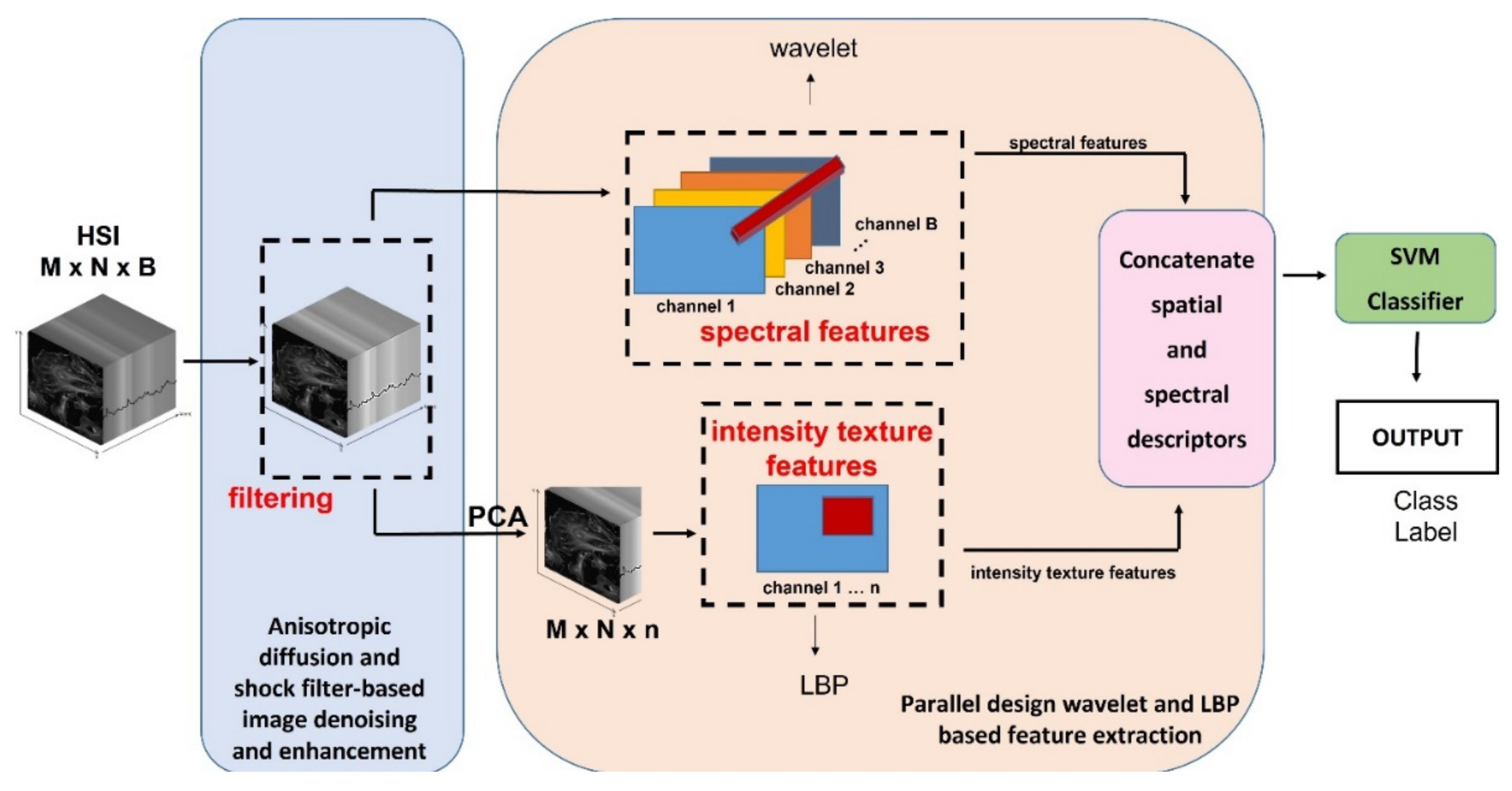
3.2. The Proposed Processing Method

The presented developed data processing workflow is depicted in Figure 2, where the three major stages of the HSI processing, along with the corresponding applied methods, are pipelined.

Briefly, in the first stage, data is filtered using an anisotropic diffusion and shock filter-based image denoising and enhancement method. For the second stage, a parallel approach [22] concatenates two feature vectors: one obtained from the wavelet transform applied in the spectral domain, and respectively, the LBP feature vector obtained from the spatial domain. For the spatial dimension, a principal component analysis is implemented in order to reduce the dimensionality of the HSI prior to the LBP. The two form the final feature vector used in the classification performed in stage 3. The figure emphasizes the independence of the two steps from one another, in the commonly referred parallel approach [22]. The SVM classifier takes the 1D concatenated feature vector and determines the correct label from the list of defined classes.

Each stage is responsible for reducing some of the known problems of HSI (e.g., noise, high intraclass variability, etc.) while contributing to increased classification performance.

3.2.1. The Spatial-Spectral Adaptive Shock Filtering Model

For hyperspectral images, the presence of noise can degrade the quality of the data, thus limiting the accuracy based on which the data is mapped to the appropriate labels. In this case, noise can damage both spatial and spectral information, generating challenges in the classification phase [18]. As in the case of classic images, the noise cancelation process for a hyperspectral image aims at the suppression of the noise on homogeneous regions while preserving the high frequency details that characterize an image in a certain band.

Throughout the paper the following notation is used: U^k—the luminance function corresponding to a band$k$, for the spatial coordinates $\left(x, y\right)$.

The proposed spatial-spectral adaptive shock filtering method was designed under the partial differential equations (PDE) framework and includes a smoothing term for non-linear noise filtering acting on the spatial dimensions and a shock filter designed to exploit the spectral dimension and to allow enhancement processes to also take part without inter-band diaphony.

The continuous model for the spatial-spectral adaptive shock filtering approach is inspired by the PDE-based fusion approach introduced in [37] and is driven in each HSI pixel by a combination between a classic anisotropic diffusion Perona Malik equation and a shock filter:

$$\frac{\partial U^k}{\partial t}=div\left(g\left(\left|\nabla U^k\right|\right)\nabla U^k\right)-\alpha \times sign\left(U_{\eta \eta }^M\right)\left|\nabla U^k\right|,$$

(2)

where:

$$M=\underset{j}{argmax}\left(\left|\nabla U^j\right|\right), j=1. . . B,$$

(3)

with $\alpha$ being the weighting factor for the enhancement term.

The first term in Equation (2) is a Perona–Malik term responsible for intra-channel denoising [20]. The second term is based on the shock filter theory, being able to inject high frequency information when discontinuities are present. In a classic formulation, for a generic luminance function U (x, y), the shock filter equation is:

$$\frac{\partial U}{\partial t}=-sign\left(U_{\eta \eta }\right)\left|\nabla U\right|,$$

(4)

with edge directions orthogonal to:

$$\eta =\frac{\nabla U}{\left|\nabla U\right|}.$$

(5)

In Equation (4), $U_{\eta \eta }^M$ represents the second order derivative in the directions orthogonal to the edges.

Depending on the sign of the second order derivative, the shock filter equation corresponds to morphological continuous erosions and dilations:

$$\frac{\partial U}{\partial t}=-\left|\nabla U\right|,$$

(6)

or:

$$\frac{\partial U}{\partial t}=\left|\nabla U\right| ,$$

(7)

producing piecewise constant regions separated by jumps [20].

In the model given by the system of Equation (2) we consider that the pertinent information is included in the spatial regions corresponding to rapid luminance function changes associated to edges and fine-scale details.

From a spatial point of view, edges or fine-scale details are filtered out or enhanced due to the first term, depending on the relationship between the spatial vector norm and a diffusion threshold K, a parameter for the classic anisotropic equation. The goal of the enhancement term is to reinforce high frequency information across the bands in which local structures are coherent. Equation (3) is used to detect, for each pixel, the band in which the spatial gradient vector norm has the highest value. For correlated local structures, the enhancement term approaches in each band a backward diffusion process and injects high frequency content and, thus, reinforces them. In case of uncorrelated structures, the high frequency information is not injected by this term in the other bands, limiting the channel mixing effects [20].

Such a filter can only be made stable in a discrete setting using slope-limiter functions. Similar to [20], we employ the min-mod function m(.):

$$m\left(x,y\right)=\left(\frac{sign\left(x\right)+sign\left(y\right)}{2}\right)\cdot min(\left|x\right|,\left|y\right|).$$

(8)

Using the notations $U_{i,j,k}^n$for denoting the luminance functions in a pixel having the spatial coordinates (i, j) in a band k at time instant n, the corresponding numerical approximation for the gradient vector norm is:

$$\left|\nabla U^k\right|=\sqrt{\begin{array}{c}{m}^2\left[D_x^{+}\left(U_{i,j,k}^n\right),D_{i,j}^{-}\left(U_{i,j,k}^n\right)\right]+\\ m^2\left[D_y^{+}\left(U_{i,j,k}^n\right),D_y^{-}\left(U_{i,j,k}^n\right)\right]\end{array}}.$$

(9)

For approximating the second order derivative:

$$U_{\eta \eta }=\frac{U_{xx}{U}_x^2+2U_{xy}{U}_x{U}_y+U_{yy}{U}_y^2}{\left|\nabla U\right|},$$

(10)

we use the classic spatial forward and backward difference operators in each band $D_x^{\pm }\left(U_{i,j,k}^n\right)$ and $D_y^{\pm }\left(U_{i,j,k}^n\right)$ for the numerical approximation on the directional derivatives, [31] and the following second-order derivatives approximations for each band:

$$\begin{array}{cc}\hfill U_{xx}{}^k& =D_x^{+}\left[D_x^{-}\left(U_{i,j,k}^n\right)\right]=D_x^{+}\left[U_{i,j,k}^n-U_{i-1,j,k}^n\right],\hfill \\ & =U_{i+1,j,k}^n-2U_{i,j,k}^n+U_{i-1,j,k }^n\hfill \end{array}$$

(11)

$$\begin{array}{cc}\hfill U_{yy}{}^k& =D_y^{+}\left[D_y^{-}\left(U_{i,j,k}^n\right)\right]=D_y^{+}\left[U_{i,j,k}^n-U_{i,j-1,k}^n\right] ,\hfill \\ & =U_{i,j+1,k}^n-2U_{i,j,k}^n+U_{i,j-1,k}^n \hfill \end{array}$$

(12)

$$U_{xy}{}^k=\frac{U_{i+1,j+1,k}^n+U_{i-1,j-1,k}^n-U_{i+1,j-1,k}^n-U_{i-1,j+1,k}^n}{4}.$$

(13)

We employ the rational Perona-Malik function and an explicit time-discretization scheme for approximating the solution of Equation (2).

We have showed preliminary results for our approach in [20] that illustrate that the proposed spatial-spectral adaptive shock filtering model for the HSI image is capable of filtering and enhancing the data, ensuring that the hyperspectral information stays loyal to its electromagnetic response for each band, without creating artefacts that may alter the information, by avoiding bands mixing in the restoration process.

Other methods, [25,27], are more widely and commonly used to enhance and filter the hyperspectral data. These will be compared in terms of experimental and visual performance in the experimental section of the paper with this proposed approach based on PDEs.

The first method is the TV (Total Variation) technique that takes into consideration only the spatial dimension of the data. In [25] it was concluded that the total variation method (TV) has good capabilities to eliminate noise, while retaining the edge information in the images. Based on those results, the TV model was also applied as a noise elimination technique for the HSI data. Even though this algorithm allows a degree of smoothness that can be adjusted to three-dimensional data, it is not a method designed specifically for the HSI pseudo-3D data.

The Combined Spatial and Spectral Weighted Hyperspectral Total Variation Model from [27] is the second method considered in the experimental evaluation, which combines the spatial and spectral dimensions. This model is based on the total variation model, with two regularization parameters, one for the spatial, and one for the spectral dimensions, supervising the reduction of the noise contained in the HSI image. This method was designed with the intent of combining the TV regularizations in the two dimensions, the spectral and the spatial one, as a unified framework, based on the pseudo-3D data format along with the dependencies between the adjacent pixels. Those refinement steps are performed by the weighted regularization terms, for the spatial dimension, and respectively for the spectral dimension. The two weighted regularization terms are capable of automatically penalizing the strength of each pixel in both the spatial and spectral dimensions. We refer to [27] for a full description of the method.

3.2.2. The Parallel Approach Based on Wavelet and LBP for Feature Extraction

As mentioned, it is relevant to take advantage of both spatial and spectral information and the dependencies between them in order to construct a jointly spatial-spectral classifier. We propose to construct a feature descriptor by independently extracting information from the spatial and spectral dimension (e.g., a parallel approach, as defined in [22]) and joining the results in the form of a concatenated vector in order to preserve both types of contexts in the labeling phase.

The local binary pattern (LBP) method, known as a powerful texture descriptor [30], is proposed to be applied to the hyperspectral data sets. The LBP is employed only on a subset of bands selected from the original high-resolution image, with the purpose of obtaining a more relevant description of the texture information present in the spatial dimension.

For a center pixel in an image$t_c$, the LBP value is computed by comparing its intensity value with its neighbors. The neighbors used for comparison are placed in a specific region with the corresponding binary label. Those labels take the following values: 0 if the centered pixel has a smaller intensity value than the neighbor or 1 otherwise, as shown in Figure 3.

The neighboring pixels are selected starting from the center pixel, from which several equally spaced samples over a circle of radius R are selected. The value of R determines the number of neighboring pixels positioned all around the center pixel.

The local binary code expressed based on the selected P neighbors [38], is defined as:

$$LB{P}_{P,R}\left( t_c\right)={\displaystyle \sum }_{i=0}^{P-1}s\left(t_i-t_c\right)2^i,$$

(14)

where$t_c$represents the intensity value of the center pixel having the coordinates $x_c \mathrm{and} y_c,$compared with each intensity value from the neighborhood represented by$t_i.$

The function s$\left(.\right)$ from Equation (14) gives the corresponding binary values for the neighboring pixels illustrated by:

$$s=\left\{\begin{array}{c}1 if t_i-t_c \ge 0 \\ 0 if t_i-t_c<0\end{array}\right..$$

(15)

When the LBP method is applied as a feature extraction technique, the set of parameters (P, R), given by the number of P neighbors distributed on a radius R, are usually defined as (8, 1), (16, 2), etc. The obtained LBP hyperspectral texture features are defined by the texture orientation and smoothness in a local region, defined by the (P, R) set. When analyzing the texture in a certain region, of the HSI data set, textures with different orientations are encountered. To avoid these issues, we propose the use of a rotation invariant uniform local binary pattern, $LB{P}_{P,R}^{riu2},$ introduced in [38]:

$$LB{P}_{P,R}^{riu2}=\min \left\{ROR\left(LB{P}_{P,R} ,i\right)\right\} | i=0,1\dots P-1,$$

(16)

where ROR($LB{P}_{P,R}$, i) is designed to perform a circular bit-wise right shift on the P-bit number of the $LB{P}_{P,R}$over a number of times proportional with the number of neighbors. The rotation invariant LBP defined in Equation (16) can quantify the statistical occurrences for each individual rotation invariant uniform pattern, represented by the superscript $riu2$, that can be included into a specific microfeature, which will result in $2^P$ different patterns capable of characterizing various texture information present in a specific band. The LBP obtained codes construct the corresponding LBP histogram of an image, as illustrated in Figure 4.

The wavelet transform is applied along the spectral dimension of the HSI data set. This means that for a selected 1D hyperspectral pixel we use the wavelet transform in order to perform a multiscale analysis of its content, by detecting the locations and scales at which significant properties of the spectral signature do exist.

We use a wavelet transform to analyze the information in a signal, at multiple scales. This analysis is done through a process based on scaling and translation, a process which gives the frequency content quantification and the time localization for a classic time-dependent signal. The process of scaling, noted as s, and translation, noted by the τ coefficient, is illustrated for the function $\psi \left(x\right)$, represented as ${\psi }_{s,}\left(x\right)$ by the formula, [39,40]:

$${\psi }_{s,}\left(t\right)=\frac{1}{\sqrt{s}}\psi \left(\frac{t-}{s}\right),$$

(17)

where $\psi \left(x\right)$ is called the wavelet or the mother function.

The wavelet transform takes a signal x(t) and decomposes it on the set of basis functions ${\psi }_{s,}\left(x\right),$ producing a time-scale representation of the same signal:

$$W_x\left(s,\right)=\underset{-\infty }{\overset{\infty }{{\displaystyle \int }}}{\psi }_{s,}\left(t\right)x\left(t\right)dt.$$

(18)

In our proposed processing pipeline, we formally consider the time dimension of a 1D wavelet to be the spectral band corresponding to a HSI image in the spectral signature. We use the discrete wavelet transform (DWT) that offers different levels of decomposition for the spectral signature content, as illustrated in Figure 5, separated in low-pass (L) and high–pass components (H) of the spectral signature of the hyperspectral image. As illustrated in Figure 5, the DWT-based wavelet processing induces a decimation operation based on an iterative process on the low-pass (L) component, which produces new low-pass and high-pass sub-bands for the illustrated hyperspectral pixel.

We used the Haar wavelet mother function in all our experiments. As illustrated in our previous work from [21], both Haar and Daubechies provide good performance results. In this paper we chose the Haar wavelet in order to reduce the border effects characteristic to wavelets.

3.2.3. The Concatenation of the Spatial and Spectral Descriptors

The parallel approach used in this paper is shown in Figure 6, where different feature descriptors, obtained independently from each other, are concatenated into a single feature vector and fed to the classifier. Preliminary results, without using the adaptive filtering approach, were included in [21] and demonstrate that, by reducing the dimensionality of the classification process, overall good accuracy, in case of random sampling-based train/test sample separation, can be obtained.

Similar to [21], spectral features (wavelet-based) and spatial features (LBP histograms) are concatenated in the last step in the feature extraction stage, to combine different representations of the data in order to obtain better classification accuracy.

The size of the feature vector varies according to the number of wavelet coefficients for the spectral features, the number of bands retained by the PCA dimensionality reduction process and the number of bins for representing the LBP histograms.

For example, for a spatial signature for $B$ bands and a single decomposition level, considering only low pass coefficients, 10 PCA hyperspectral bands and an LBP operator with P neighbors, the corresponding feature vector size is $B/2+10 x (P+1$); for both low pass and high pass wavelet coefficients the corresponding feature vector size will be $B+10 x \left(P+1\right).$

3.2.4. Controlled Sampling for Classification Accuracy Estimation

Most of the supervised hyperspectral image classification approaches are designed to classify the hyperspectral pixels, or the dimensional vectors from the same class. Those vectors, if they are from the same classes, have similar spectral responses or spectral-spatial features. Based on these assumptions, a trained classifier can be generalized to predict the labels of unseen samples, known as the testing data set. However, this concept does not always hold if the training and testing samples are not carefully selected. In the case of supervised classification, the traditional design for spectral classification leads to unfair or biased performance evaluation that are, generally, caused by the way the training and testing samples are selected, usually by a random partition of the hyperspectral data set. The phenomenon was already identified in experimental setups dealing with deep learning networks and HSI for joint spatial-spectral processing, where a comparison between random selection of samples versus spatially disjoint sample selection was performed. The conclusions demanded for more investigation of the matter. Details of this can be found in [7]. This practice is used in order to compensate for the limited availability of benchmark data and the high cost of having a large number of reference maps in the data collection.

Choosing the samples in an arbitrary, or random way from a data set results in dependence between the samples in the training and testing data sets. In the case of hyperspectral images, this sampling strategy, based on random selection, biases the results, since testing samples may be located adjacent in terms of spatial position to the training ones. So, the independence assumption between the two data sets, is flawed due to the spatial correlation between the training and the testing samples [41].

As pointed out earlier, when discussing about the classification of the spectral-spatial information, one must be careful when selecting the training and testing samples, in such a way that the data sets do not interact with each other. The problem of overlapping pixels from different classes is illustrated in Figure 7a. The emphasis here is on the fact that spatial processing also considers the neighboring pixels, and, depending on the size of the window/kernel used, with a random selection of the training data, or even with a spatially disjoint approach (due to boundary effects), there is a random number of pixels that have overlapping areas, faulting the independence assumption between the training and testing data samples.

This overlapping phenomenon generally results in exaggerated classification accuracy. Such, the information from the testing data set could be used in the training step by spatial operations, leading to a biased evaluation result, leading to the need for the implementation of a controlled sampling strategy. When using patch-based representation, as in [23], the independence between the training set and the testing set must be considered.

To address the overlapping problem due to the applied spatial operations, a proposed controlled partitioning is considered, as illustrated in Figure 7b.

By analyzing Figure 7a, one can observe that the two windows having the centered red and blue pixels overlap. This overlapping can occur, for example in the case of the LBP method applied on the spatial dimension. The LBP method is designed to determine the LBP histograms for each pixel based on a square patch, as already shown in Figure 4. The dimension of the window, along with the proximity of the selected samples, determine an unbiased performance result. This is due to the similarity between the two pixels, since the concatenated histograms along the spectral dimension, representing the feature vector, being almost identical, will determine the biased classification results, in the learning phase and in the testing phase.

A relevant controlled sampling strategy should have the capability to avoid selecting samples homogeneously over the whole image and it also must penalize overlapping between the data sets. It should also ensure that the selected training samples are representative for each class. Even though there are many samples in a specific class, those samples can vary slightly between one another, helping for a better labeling of the data, due to variation in the spectral dimension. Based on [35], and considering the aforementioned arguments, the explanations and details of the proposed method are described below:

Input: HSI data set U, the sampling rate ratio (the number of samples/percentage per class, the reference map, the desired distance between the pixels, the window representing the populated neighborhood

Output: training data set X_train

For each class c in U:

Determine all the partitions X in class C

For each partition x in X:

Get the centroid for each region in the partition

Get the spatial coordinates $\left(i, j\right)$ of the corresponding centroid

Calculate the number of training samples tot in the partition:

no_of_desired_samples = tot * ratio

While visited register is empty:

Add the samples situated at an established distance from the centroid and from the previous added sample

After each insertion of a sample in visited register, we verify:

if visited <= no_of_desired_samples; if not, continue with the region growing algorithm based on a window dimension representing the populated neighborhood

End while

End for Combine all the visited registers from the corresponding regions for the training samples End for

Combine all the samples from the partitions to obtain the final X_train training data set.

As a starting point for the proposed controlled sampling strategy, all the seed points are randomly selected from different partitions of the classes. Then, the controlled sampling process proceeds as follows: first, one must consider the different spatial positions of each class, so one must determine for each partition, the positions for all the labels from which the samples are selected.

The next step determines the distance at which each sample is selected, based on the position of the previous selected one, making sure that the selected training samples cover the spectral variance. This process is repeated until the number of selected points reaches a predefined number or a ratio. After the samples are extracted for each individual class, based on the expanding region already defined, given by a specified window, the neighborhoods are constructed based on the specific window size. The process is repeated until the training data set is selected.

4. Results

4.1. Hyperspectral Datasets

We performed experiments on the publicly available data sets [42]: Indian Pines, Pavia University and Salinas. The class distribution of the scenes is presented in Figure 8 for the Indian Pines dataset, Figure 9 for the Pavia University dataset and Figure 10 for the Salinas dataset, with the corresponding distributions of samples per class, based on the proposed controlled sampling strategy and the corresponding window size for the neighborhood construction.

The Indian Pines dataset was captured over an agricultural area in 1992 by the AVIRIS sensor and is characterized by the presence of crops of regular geometry and irregular forest groups. The reference dataset available is divided into 16 classes with 10,249 labeled pixels overall. The Pavia University contains nine different classes belonging to an urban environment with multiple solid structures, natural objects and shadows captured by the ROSIS sensor. The Salinas data set is also captured by the AVIRIS sensor and consists of data over several agricultural fields. The reference data is made up of 42,776 labeled pixels (from a total of approx. 200,000). More details on the number of independent samples per class for supervised learning are given in Section 4.2.

The Indian Pines scene is represented by a size of 145 × 145 and 200 spectral bands. The Salinas scene has 204 spectral bands, with a dimensionality of 512 lines and 217 samples. The Pavia University scene is composed of 103 bands, with the dimension of 610 × 340 pixels.

4.2. Ensuring the Independence between Data Training and Data Testing

The results for the proposed processing pipeline for the HSI classification depend greatly on the manner in which the data training and data testing steps are constructed. This means that the classification accuracy strongly depends on the number of training samples and how those sampled are selected with respected to the remaining ones.

We propose and evaluate the controlled sampled strategy for two different neighborhoods sizes: one for a window size of 3x3 (w3) and one for a window size of 5 × 5 (w5). In Figure 11 the constructed neighborhoods with the corresponding distance between them are depicted. The three points, A, B and C, represent the samples selected for the training dataset. In this representation we have singular pixels selected as samples used in the learning phase, distributed at equal distances based on the dimension of the desired window size.

In Figure 12 we illustrate for comparison the two strategies for selecting the samples: a random strategy and the proposed controlled strategy for a better understanding of the proposed method. One can observe that it is difficult to ensure the independence between the training and data sets for the random selection.

4.3. The Experimental Configuration

We evaluate the performance in classification of the proposed end-to-end processing pipeline for HSI using a validation approach similar to the one in [25]: the number of the PCA selected bands was fixed to 10, and the patch size used for computing the histograms of the LBPs were set to 3 × 3 and 5 × 5 for all the datasets. The window sizes for the proposed controlled sampling strategy were set to 3, respectively 5, corresponding to the selected neighborhood dimensions, of w = 3, respectively, of w = 5. When we considered the selected window for the controlled strategy as 3 × 3, the distance between the centered neighborhoods is therefore 5. If we considered the windows to be 5 × 5, then the distance between the center of the neighborhood is 7. For the denoising and enhancing method, the parameters used in paper [20] were kept for each data set, the number of iterations depending on the complexity of the stored information in the HSI.

The same window size was used for all the experiments dealing with the LBP histogram computation. To ensure the independence between the training and testing samples, the proposed controlled sampling strategy, grouped as the collected samples based on neighborhoods, situated at certain distances. This determined a selection of a smaller number of samples per class in comparison with a random strategy approach.

We used the LBP feature descriptors for which a histogram of LBP values on a patch centered on a given pixel was created. The rotational invariant LBP model uses different values for the set of parameters (P, R), like (8,1) or (16,2). The corresponding distance between the neighborhoods of the selected training samples ensures a minimal overlapping of the LBP histogram computation to ensure the independence between the training and the data sets.

The feature vector, for each pixel in the data cube, is built by concatenating the patch histograms of each band along with the spectral wavelet features, and then fed into the SVM classifier to evaluate the overall accuracy of the processing pipeline.

Table 1. Size of the feature vector fed into the SVM for Indian Pines having 200 bands, for N = 1 and N = 2 wavelet decomposition levels.

Number of Bands after the PCA Band Reduction Process (n1)	Number of Neighbors (Param. P of LBP) (n2)	Spatial Features	Spectral Features	Size of the Feature Vector
		Number of LBP Histogram Bins (nbins)	Wavelet Level
10	8	9	N = 1 (L)	100	190
			N = 2 (LL)	50	140

illustrates how the size of the feature vector fed into the SVM is determined.

To evaluate the classification performance of the proposed architecture, we compared the obtained results with the state-of-the-art support vector machine (SVM) classifier, with the radial basis function (RBF) kernel, where gamma has the value 0.001 and the regularization parameter c is set to 200. The corresponding parameters for SVM were obtained through a grid search for each data set. For the wavelet filters, an important parameter is represented by the level of decomposition (N) which gives the number of components of the hyperspectral vector for the spectral domain. Therefore, considering different decomposition levels, the wavelet filter can extract the desired features from the input for a better representation of the signal. In this paper, we denote for the first level decomposition (N = 1) the low (L) coefficients to$cA$. Similar, for the second level of decomposition (N = 2) the low (LL) coefficients are represented by the same $cA$ notation. For the third level of decomposition (N = 3), we combine the low (LLL) coefficients, represented by the same $cA$, with the high (LLH) coefficients denoted in this situation as $cD$.

We illustrate the performance of the proposed model for three decomposition levels, N = 1, N = 2 and N = 3. Alongside the three levels, we have chosen for the first two levels only the low (L) coefficients, denoted as cA, and for the third level, we have chosen to concatenate the complete low pass coefficients with the high pass (H) coefficients. For N = 3 levels, the high coefficients are denoted as cD.

4.4. Obtained Experimental Results

For all the experiments, we used the overall accuracy (OA) evaluation as a measurement of how well the proposed processing pipeline behaves, along with the controlled strategy and how this can increase the classification performance. In this case, the OA represents the number of correctly classified samples. The performance results were averaged over 10 experiments.

We tested the performance of the proposed three stage pipeline: data denoising and enhancement, feature extraction followed by data classification. We tested the data filtering and enhancement techniques based on the shock filters and compared it with the results obtained from the TV and the CSSWHTV methods. After each filtering method, we extracted the spatial and spectral features. At the end of the concatenation step, the classifier analyzed the spatial-spectral concatenated features to establish the corresponding label for each feature vector.

The obtained results are presented according to the validation they bring to the end-to-end approach, starting from the introduction of the controlled sampling strategy, continuing with the illustration of the influence of either dimension of the data (e.g., spatial and spectral) to the classification. This approach follows the most appropriate feature selection combination for the parallel approach (where spectral and spatial descriptors are combined) and illustrates the added value brought by the denoising and enhancement stage. We include in the manuscript the gradual improvements added by each of the proposed methods and reach the processing pipeline described in Figure 2 referring to the Indian Pines dataset. Then, we provide, for comparison, the results for all the datasets in Section 4.1.

4.4.1. Random Sampling vs. Controlled Sampling Evaluation

To understand the influence of the sampling strategy on the classification and the bias introduced when there is no control over the independence between the test and the training dataset partition, for different window sizes, w = 3, w = 5, and w = 11, we performed a classification of the Indian Pines dataset experiment using a random sampling strategy. Results are illustrated in

Table 2. Classification accuracy (OA) using the random sampling, for the Indian Pines dataset, with different windows size, of dimension 3 × 3, 5 × 5 and 11 × 11, for the LBP histogram computation.

Feature Extraction Method		Window Size
		w3	w5	w11
$\mathrm{LBP}\mathrm{method}$ $\mathrm{only}$	${\mathrm{LBP}}_{8,1}^{\mathrm{riu}2}$	75.35 ± 1.42	97.69 ± 1.81	98.19 ± 0.71
	${\mathrm{LBP}}_{16,2}^{\mathrm{riu}2}$	77.09 ± 1.67	97.30 ± 1.24	99.93 ± 0.55

.

The high values of the obtained results, as the size of the window increases, are associated to an increasing similarity between the test and training dataset used, in the case of a window size of 11 × 11, challenging the random partitioning approach.

In all subsequent experiments we used our controlled sampling strategy for the validation of the results.

4.4.2. Spatial vs. Spectral Information for Feature Extraction

Next, we tested the influence of independently considering the spatial information and the spectral information to classify the Indian Pines dataset. The approach aimed at validating the usage of a control sampling strategy, capable of decorrelating and ensuring independence between samples in the spatial dimension of the data.

As illustrated in

Table 3. Classification accuracy (OA) for the Indian Pines dataset with different windows size, of dimension 3 × 3 and 5 × 5, for the controlled sampling strategy, without filtering, using the window size for the LBP histogram computation, or the wavelet transform on three levels, with low pass coefficients (cA), respectively high pass coefficients (cD).

Methods and Corresponding Parameters		Window Size
		w = 3	w = 5
$\mathrm{LBP}\mathrm{method}$ $\mathrm{only}$	${\mathrm{LBP}}_{8,1}^{\mathrm{riu}2}$	25.74 ± 1.21	26.27 ± 0.99
	${\mathrm{LBP}}_{16,2}^{\mathrm{riu}2}$	25.74 ± 1.29	26.27 ± 1.32
$\mathrm{Wavelet}\mathrm{method}$ $\mathrm{only}\mathrm{for}\mathrm{the}\mathrm{three}\mathrm{levels}$	N = 1 (cA)	76.40 ± 1.52	75.68 ± 1.78
	N = 2 (cA)	76.85 ± 1.98	78.05 ± 1.78
	N = 3 (cA + cD)	80.52 ± 1.18	74.91 ± 1.27

, for the controlled sampling strategy presented in this paper, when we use only the LBP histogram, we do not have high classification rates.

When we use the wavelet method, compared with the LBP one, we have a significant increase in classification performance, independent of the window size desired. However, spatial information is still relevant to the classification.

4.4.3. Parallel Spatial-Spectral Feature Extraction and Classification

Based on the processing pipeline presented in this paper, we test different options of combining the spectral and spatial features extracted by a parallel approach to improve the quality of the overall feature vectors for the HSI data. The obtained results are presented in

Table 4. Classification accuracy for the Indian Pines dataset, without filtering, with wavelet transform up to three levels, with the corresponding window size, of dimension 3 × 3 and 5 × 5, for the controlled sampling strategy and LBP histogram computation, w3 and w5 (OA).

	Spectral Feature		Window Size
Spatial feature	Wavelet Level	High/Low Pass Coefficients	w3	w5
${\mathrm{LBP}}_{8,1}^{\mathrm{riu}2}$	N = 1	cA	84.49 ± 1.54	83.62 ± 1.78
	N = 2	cA	83.45 ± 1.32	82.42 ± 1.69
	N = 3	cA + cD	81.59 ± 1.25	78.04 ± 2.12
${\mathrm{LBP}}_{16,2}^{\mathrm{riu}2}$	N = 1	cA	84.98 ± 1.82	84.54 ± 1.89
	N = 2	cA	84.10 ± 1.63	82.41 ± 1.33
	N = 3	cA + cD	83.23 ± 1.47	72.24 ± 1.85

for the Indian Pines dataset without filtering.

The table illustrates the importance of combining the spectral and spatial information, leading to better classification results obtained under the same conditions for the training and testing selection of the data, compared to the previous case in Table 2 when only one dimension was considered.

4.4.4. Contribution of the Data Filtering for End-to-End Classification

Finally, we included a filtering step to further improve our results, according to the proposed end-to-end parallel approach.

The classification results based on the proposed framework are presented in

Table 5. Classification accuracy for the Indian Pines dataset, using the TV, the CSSWHTV and the anisotropic diffusion and shock filter-based approaches, with wavelet transform for three levels, with the corresponding window size, of dimension 3 × 3 and 5 × 5, for the controlled sampling strategy and LBP histogram computation, w3 and w5 (OA).

Filtering Method	Spatial Feature	Spectral Feature		Window Size
		Wavelet Level	High Pass (cD)/Low Pass (cA) Coeff.	w3	w5
TV filtering	${\mathrm{LBP}}_{8,1}^{\mathrm{riu}2}$	N = 1	cA	90.2 ± 1.3	87.83 ± 0.96
		N = 2	cA	88.16 ± 0.92	86.69 ± 1.62
		N = 3	cA + cD	80.99 ± 1.45	82.95 ± 1.55
	${\mathrm{LBP}}_{16,2}^{\mathrm{riu}2}$	N = 1	cA	90.36 ± 0.96	88.12 ± 1.02
		N = 2	cA	88.24 ± 1.78	86.45 ± 1.63
		N = 3	cA + cD	81.1 ± 1.65	83.15 ± 1.54
CSSWHTV filtering	${\mathrm{LBP}}_{8,1}^{\mathrm{riu}2}$	N = 1	cA	86.46 ± 1.26	84.56 ± 1.65
		N = 2	cA	84.12 ± 1.24	82.83 ± 1.28
		N = 3	cA + cD	74.73 ± 1.96	83.03 ± 1.63
	${\mathrm{LBP}}_{16,2}^{\mathrm{riu}2}$	N = 1	cA	86.46 ± 1.62	84.56 ± 1.21
		N = 2	cA	84.12 ± 0.76	82.83 ± 1.03
		N = 3	cA + cD	74.73 ± 1.26	83.03 ± 1.69
proposed anisotropic diffusion and shock filter	${\mathrm{LBP}}_{8,1}^{\mathrm{riu}2}$	N = 1	cA	93.85 ± 1.57	90.04 ± 0.99
		N = 2	cA	91.38 ± 1.2	89.4 ± 1.85
		N = 3	cA + cD	81.64 ± 1.87	85.95 ± 1.27
	${\mathrm{LBP}}_{16,2}^{\mathrm{riu}2}$	N = 1	cA	93.37 ± 1.25	90.73 ± 1.12
		N = 2	cA	91.53 ± 1.22	88.84 ± 1.28
		N = 3	cA + cD	83.25 ± 1.98	85.88 ± 1.22

. Each corresponding table depicts the results obtained by one of the three filtering techniques. By analyzing the results, we observe that there is only a slight difference in performance when comparing the results from $LB{P}_{8,1}^{riu}$ and $LB{P}_{16,2}^{riu}$.

One can observe that the shock filtering method performs better in comparison with the TV and CSSWHTV methods, also in terms of visual results for the classification maps (Figure 13d) and in terms of the confusion matrices (Figure 14c). Moreover, when compared in terms of overall classification results based on different window sizes, w3 and w5, there is an increase in performance with smaller window size. We attribute this to the larger number of samples per class in the case of a window of size 3, compared to 5. Figure 13 shows the classification maps for the three filtering methods, for the ${\mathrm{LBP}}_{8,1}^{\mathrm{riu}2}$ with an N = 1 number of wavelet decomposition levels. Figure 14 presents the corresponding confusion matrices.

We include also the confusion matrix in order to provide more insights about the classification accuracy especially when dealing with imbalanced datasets due to the original sample distribution or to the number of resulting samples after applying the controlled sampling strategy. We used it to compute the mean accuracy in

Table 6. Average accuracy performance per class (%), for the Indian Pines dataset, for the TV, the CSSWHTV and the anisotropic diffusion and shock filter methods, with a controlled sampling based on the 3 × 3 (w3) window size for the training set, N = 1 wavelet transform level and ${\mathrm{LBP}}_{8,1}^{\mathrm{riu}2}.$

Indian Pines Class Name	Average Accuracy for Each Method
	TV(%)	CSSWHTV (%)	Anisotropic Diffusion (%)
Corn-notill	87.54	81	90.09
Corn-mintill	87.91	76.37	91.76
Grass-pasture	95.9	92.43	95.9
Grass-trees	97.37	96.24	99.06
Hay-windrowed	98.27	99.14	99.71
Soybean-notill	70.91	67.84	70.18
Soybean-mintill	90.42	85.03	92.79
Soybean-clean	93.4	87.07	95.25
Woods	99.12	98.75	99.37

to assess the classifier performance on each class.

Results in Table 6 regarding the obtained results in terms of the Average accuracy (AA) performance per class validate that there is no major difference due to the available number of samples among classes.

4.4.5. Classification Results on the Salinas Datasets

The classification results based on the proposed model for the Salinas dataset are presented in

Table 7. Classification accuracy for the Salinas dataset, using the TV, the CSSWHTV and the anisotropic diffusion and shock filter-based approaches, with wavelet transform for three levels, with the corresponding window size, of dimension 3 × 3 and 5 × 5, for the controlled sampling strategy and LBP histogram computation, w3 and w5 (OA).

Filtering Method	Spatial Features	Spectral Feature		Window Size
		Wavelet Level	High Pass (cD)/Low Pass (cA) Coeff.	w3	w5
TV filtering	${\mathrm{LBP}}_{8,1}^{\mathrm{riu}2}$	N = 1	cA	94.1 ± 1.45	93.59 ± 1.87
		N = 2	cA	93.88 ± 1.85	93.45 ± 1.48
		N = 3	cA + cD	92.78 ± 1.89	95.7 ± 1.75
	${\mathrm{LBP}}_{16,2}^{\mathrm{riu}2}$	N = 1	cA	94.85 ± 1.42	93.77 ± 1.49
		N = 2	cA	93.56 ± 1.85	93.41 ± 1.47
		N = 3	cA + cD	95.93 ± 1.45	92.67 ± 1.81
CSSWHTV filtering	${\mathrm{LBP}}_{8,1}^{\mathrm{riu}2}$	N = 1	cA	92.82 ± 1.98	92.67 ± 1.52
		N = 2	cA	92.81 ± 1.84	92.67 ± 1.22
		N = 3	cA + cD	90.68 ± 1.14	92.13 ± 1.87
	${\mathrm{LBP}}_{16,2}^{\mathrm{riu}2}$	N = 1	cA	92.99 ± 1.48	92.81 ± 1.47
		N = 2	cA	92.47 ± 1.85	92.12 ± 1.36
		N = 3	cA + cD	91.62 ± 1.58	92.69 ± 1.74
proposed anisotropic diffusion and shock filter	${\mathrm{LBP}}_{8,1}^{\mathrm{riu}2}$	N = 1	cA	95.41 ± 1.22	95.1 ± 1.22
		N = 2	cA	95.49 ± 1.82	94.71 ± 1.56
		N = 3	cA + cD	94.36 ± 1.32	94.1 ± 1.75
	${\mathrm{LBP}}_{16,2}^{\mathrm{riu}2}$	N = 1	cA	96.54 ± 1.87	94.91 ± 1.78
		N = 2	cA	95.88 ± 1.45	93.89 ± 1.36
		N = 3	cA + cD	93.78 ± 1.61	93.22 ± 1.55

, illustrating the results for one of the three filtering techniques. By analyzing the results, one can observe that there is only a slight difference in performance when the results from $LB{P}_{8,1}^{riu2}$ and $LB{P}_{16,2}^{riu2}$ are compared.

A difference in classification performance can be observed based on the selected filtering method. The shock filtering method brings an increase in performance, by ~2% when compared with the TV method and ~3% when compared with the CSSWHTV method. The visual results for the Salinas dataset, in terms of classification maps, based on the different filtering methods used, are presented in Figure 15.

4.4.6. Classification Results on the Pavia University Datasets

The classification results based on the proposed model for the Pavia University dataset are presented in

Table 8. Classification accuracy for the Pavia University dataset, using the TV, the CSSWHTV and the anisotropic diffusion and shock filter-based approaches, with wavelet transform for three levels, with the corresponding window size, of dimension 3 × 3 and 5 × 5, for the controlled sampling strategy and LBP histogram computation, w3 and w5 (OA).

Filtering Method	Spatial Feature	Spectral Feature		Window Size
		Wavelet Level	High Pass (cD)/Low Pass (cA) Coeff.	w3	w5
TV filtering	${\mathrm{LBP}}_{8,1}^{\mathrm{riu}2}$	N = 1	cA	84.02 ± 1.52	83.86 ± 1.42
		N = 2	cA	88.29 ± 1.77	83.25 ± 1.33
		N = 3	cA + cD	82.93 ± 0.99	82.01 ± 1.02
	${\mathrm{LBP}}_{16,2}^{\mathrm{riu}2}$	N = 1	cA	85.51 ± 1.47	82.25 ± 1.41
		N = 2	cA	87.62 ± 1.78	82.45 ± 1.30
		N = 3	cA + cD	82.85 ± 1.31	82.07 ± 1.52
CSSWHTV filtering	${\mathrm{LBP}}_{8,1}^{\mathrm{riu}2}$	N = 1	cA	89.86 ± 1.52	85.91 ± 1.28
		N = 2	cA	88.4 ± 1.27	82.66 ± 1.34
		N = 3	cA + cD	83.73 ± 1.87	83.98 ± 1.85
	${\mathrm{LBP}}_{16,2}^{\mathrm{riu}}$	N = 1	cA	89.16 ± 1.74	84.88 ± 1.51
		N = 2	cA	87.25 ± 1.31	83.62 ± 1.78
		N = 3	cA + cD	83.96 ± 1.88	82.11 ± 1.39
proposed anisotropic diffusion and shock filter	${\mathrm{LBP}}_{8,1}^{\mathrm{riu}2}$	N = 1	cA	92.86 ± 1.32	91.41 ± 1.78
		N = 2	cA	92.29 ± 1.99	90.98 ± 1.22
		N = 3	cA + cD	91.75 ± 1.18	89.89 ± 1.54
	${\mathrm{LBP}}_{16,2}^{\mathrm{riu}2}$	N = 1	cA	92.12 ± 1.94	90.27 ± 1.83
		N = 2	cA	90.51 ± 1.15	89.15 ± 1.48
		N = 3	cA + cD	90.02 ± 1.54	87.32 ± 1.52

. By analyzing the results, one can observe that there is only a slight difference in performance when the results from $LB{P}_{8,1}^{riu}$ and $LB{P}_{16,2}^{riu}$ are compared.

The Pavia University data set is represented by a multitude of small structures, for which it is difficult to ensure a vast representation of samples grouped in neighborhoods. Even though the structure of the data set is represented in this way, an increase in performance is ensured by the proposed processing pipeline.

The visual results for the Pavia University, based on the different filtering methods used, are presented in Figure 16, in terms of classification maps. A difference in classification performance can be observed considering the selected filtering method. The same behavior remains for this data set as in the case of the previous two analyzed datasets: the shock filtering method can bring an increase in the performance by ~8% when compared with the TV method and by ~4% when compared with the CSSWHTV method. The analysis of the classification performance shows that the type of content in the data set influences the results for the specific controlling sampling strategy proposed.

5. Discussion

The results obtained in Table 2, under the same experimental conditions for the data set, when we consider a random sampling strategy, show higher classification rates compared with the values presented in Table 3. The disadvantage in this situation, is represented by the inability to ensure the independence between the two data sets, for training, respectively testing, which determines the network to learn and validate approximatively the same samples each time. In addition, when we increase the window size, the samples selected have a larger proportion of overlapping between each other.

In Table 4 we present the classification results obtained for the Indian Pines dataset, when data is unfiltered. Table 5 illustrates the importance of the filtering phase, its absence leading to significantly lower classification results obtained under the same conditions for the training and testing selection of the data. The shock filtering method brings an increase in performance, by ~3% when compared to the TV method, by ~6% when compared to the CSSWHTV method and by ~8% when compared to the case when no filtering was used. Based on these results, we conclude that a relevant filtering and enhancing stage brings significant contributions to the selected features for the spatial and spectral dimensions.

In general, but also in the case of deep learning methods, one could increase the overall performance of the model by adopting a random sampling strategy, as illustrated and presented in Figure 12. Regarding this random strategy, we performed the same classification of the data, after passing it through the proposed framework, using the TV filtering method. For the Indian Pines dataset, with random sampling, by selecting the corresponding number of samples per class corresponding with the window size of w3, we obtained ~95.53% accuracy, a significantly larger value in comparison with the proposed controlled sampling where we obtain ~90.02% accuracy, as seen in Table 5.

By analyzing the difference in performance of the data sets, of approximately 5%, one can initially deduce that the random sampling offers better results in terms of performance. However, this is not entirely correct, due to the fact that one cannot ensure that there is independence between the training and the testing data sets. In addition, as we increase the window size for the LBP histogram calculation, we have more overlapping between the windows, generating results with ~98–99% accuracy (see Table 2), which cannot be considered as a valid classification choice due to the bias in the experiment introduced by similarities between the samples in the training and testing data sets.

Compared to existing deep learning methods, where HSI data is directly fed to the neural network, our proposed work and sampling method provides better results.

Table 9. Classification accuracy of the proposed method compared to deep learning methods reported in the literature.

Model Name	Indian Pines Dataset	Pavia University Dataset
CNN2D40 with disjoint sample selection (results taken from [7])	82.97	84.98
CNN3D with disjoint sample selection (results taken from [7])	79.58	86.82
Proposed end-to-end (results taken from Table 5 and Table 7)	93.85	92.86

summarizes the differences in performance (in terms of OA).

We also tested the performance of the spatially disjoint method presented in [7] for training and testing distribution according to our proposed controlled sampling strategy, using the code provided by the authors, and we obtained an overall accuracy of 77.35% for the Indian Pines data set.

6. Conclusions

We proposed a processing pipeline for hyperspectral images based on three stages: filtering and enhancing, followed by feature extraction designed to take into consideration both the spatial and spectral dimension, and ending with the classification stage. Along with the proposed architecture designed to deal with the high dimensional data, we presented a controlled sampling strategy, based on the need to ensure the independence between the training data set and the testing data set, guaranteeing validity in the interpretation of the classification results when the available data set is relatively small in sample number count. We demonstrated the fact that the structure of the datasets and the elements used for representing the information has an influence on the performance of the classifier as well, where all dimension in the data need to be considered consistently: both the spatial or the geometry of the objects in the scene and their spectral representation. The experimental results illustrated the importance of the filtering and enhancing step for the hyperspectral image, even if we had a smaller number of samples per class. The anisotropic diffusion and shock filter-based proposed approach technique gave the best results in classification compared with the CSSWHTV or TV methods. A decrease in classification performance was observed when the filtering phase was eliminated, so one can conclude that the filtering and enhancement step was of foremost importance and relevance. In addition, a controlled sampling strategy, like the proposed one, defined by the two parameters, the distance between the selected samples, and the window sizes, was critical for ensuring the independence between the two data sets (training and testing) used in the classification phase and obtaining results that were not biased.

We also showed that the proposed work outperformed the reported results in the state-of-the-art using joint spectral and spatial information processing and deep-learning architectures. However, further investigation needs to be made on how the proposed controlled sampling strategy can be used together with CNN based methods, especially within the challenge of even smaller sample populations.

References

1. Chang, C.-I. Hyperspectral Imaging: Techniques for Spectral Detection and Classification; Springer Science & Business Media: New York, NY, USA, 2003; Volume 1. [Google Scholar]
2. Liang, G.; Smith, R.T. Optical hyperspectral imaging in microscopy and spectroscopy—A review of data acquisition. J. Biophotonics 2015, 8, 441–456. [Google Scholar]
3. Que, D.; Li, B. Medical images denoising based on total variation algorithm. In Proceedings of the International Conference on Environment Science and Biotechnology ICESB, Maldives, Spain, 25–26 November 2011; Volume 23, p. 227. [Google Scholar]
4. Signoroni, A.; Savardi, M.; Baronio, A.; Benini, S. Deep learning meets hyperspectral image analysis: A multidisciplinary review. J. Imaging 2019, 5, 52. [Google Scholar] [CrossRef] [PubMed] [Green Version]
5. Teke, M.; Deveci, H.S.; Haliloglu, O.; Gürbüz, S.Z.; Sakarya, U. A short survey of hyperspectral remote sensing applications in agriculture. In Proceedings of the 2013 6th International Conference on Recent Advances in Space Technologies (RAST), Istanbul, Turkey, 12–14 June 2013; pp. 171–176. [Google Scholar]
6. Adão, T.; Hruška, J.; Pádua, L.; Bessa, J.; Peres, E.; Morais, R.; Sousa, J.J. Hyperspectral Imaging: A Review on UAV-Based Sensors, Data Processing and Applications for Agriculture and Forestry. Remote Sens. 2017, 9, 1110. [Google Scholar] [CrossRef] [Green Version]
7. Paoletti, M.; Haut, J.; Plaza, J.; Plaza, A. Deep learning classifiers for hyperspectral imaging: A review. ISPRS J. Photogramm. Remote Sens. 2019, 158, 279–317. [Google Scholar] [CrossRef]
8. Fei, B. Hyperspectral imaging in medical applications. In Data Handling in Science and Technology; Elsevier: Amsterdam, The Netherlands, 2020; Volume 32, pp. 523–565. [Google Scholar]
9. Khan, M.J.; Khan, H.S.; Yousaf, A.; Khurshid, K.; Abbas, A. Modern Trends in Hyperspectral Image Analysis: A Review. IEEE Access 2018, 6, 14118–14129. [Google Scholar] [CrossRef]
10. Rasti, B.; Scheunders, P.; Ghamisi, P.; Licciardi, G.; Chanussot, J. Noise Reduction in Hyperspectral Imagery: Overview and Application. Remote Sens. 2018, 10, 482. [Google Scholar] [CrossRef] [Green Version]
11. Gómez-Chova, L.; Tuia, D.; Moser, G.; Camps-Valls, G. Multimodal Classification of Remote Sensing Images: A Review and Future Directions. Proc. IEEE 2015, 103, 1560–1584. [Google Scholar] [CrossRef]
12. Bowker, D.E. Spectral Reflectances of Natural Targets for Use in Remote Sensing Studies; NASA: Washington, DC, USA, 1985; Volume 1139. [Google Scholar]
13. Hughes, G.F. On the mean accuracy of statistical pattern recognizers. IEEE Trans. Inf. Theory 1968, 14, 55–63. [Google Scholar] [CrossRef] [Green Version]
14. Zhang, X.; Cui, J.; Wang, W.; Lin, C. A Study for Texture Feature Extraction of High-Resolution Satellite Images Based on a Direction Measure and Gray Level Co-Occurrence Matrix Fusion Algorithm. Sensors 2017, 17, 1474. [Google Scholar] [CrossRef] [Green Version]
15. Gomez, C.; Drost, A.; Roger, J.-M. Analysis of the uncertainties affecting predictions of clay contents from VNIR/SWIR hyperspectral data. Remote Sens. Environ. 2015, 156, 58–70. [Google Scholar] [CrossRef] [Green Version]
16. Engesl, J.M.; Chakravarthy, B.L.; Rothwell, D.; Chavan, A. SEEQ™ MCT wearable sensor performance correlated to skin irritation and temperature. In Proceedings of the Annual International Conference of the IEEE Engineering in Medicine and Biology Society, Milan, Italy, 25–29 August 2015; IEEE: Piscataway, NJ, USA, 2015; pp. 2030–2033. [Google Scholar]
17. Jia, S.; Jiang, S.; Lin, Z.; Li, N.; Xu, M.; Yu, S. A survey: Deep learning for hyperspectral image classification with few labeled samples. Neurocomputing 2021, 448, 179–204. [Google Scholar] [CrossRef]
18. Mohan, B.K.; Porwal, A. Hyperspectral image processing and analysis. Curr. Sci. 2015, 108, 833–841. [Google Scholar]
19. Taskin, G.; Kaya, H.; Bruzzone, L. Feature Selection Based on High Dimensional Model Representation for Hyperspectral Images. IEEE Trans. Image Process. 2017, 26, 2918–2928. [Google Scholar] [CrossRef] [PubMed]
20. Miclea, A.; Borda, M.; Terebes, R.; Meza, S. Hyperspectral Image Enhancement using Diffusion and Shock Filtering Techniques. In Proceedings of the 2019 E-Health and Bioengineering Conference (EHB), Iasi, Romania, 21–23 November 2019; pp. 1–6. [Google Scholar]
21. Miclea, A.; Terebes, R. A Novel Local Binary Patterns and Wavelet Transform-based Approach for Hyperspectral Image Classification. Acta Teh. Napoc. 2021, 61, 29–34. [Google Scholar]
22. Cernadas, E.; Delgado, M.F.; González-Rufino, E.; Carrión, P. Influence of normalization and color space to color texture classification. Pattern Recognit. 2017, 61, 120–138. [Google Scholar] [CrossRef]
23. Willett, R.; Krishnamurthy, K.; Raginsky, M. Multiscale photon-limited spectral image reconstruction. SIAM J. Imaging Sci. 2010, 3, 619–645. [Google Scholar]
24. Shen, H.; Yuan, Q.; Zhang, L. Hyperspectral image denoising employing a spectral-spatial adaptive total variation model. IEEE Trans. Geosci. Remote Sens. 2012, 50, 3660–3677. [Google Scholar]
25. Rudin, L.I.; Osher, S.; Fatemi, E. Nonlinear total variation based noise removal algorithms. Phys. D Nonlinear Phenom. 1992, 60, 259–268. [Google Scholar] [CrossRef]
26. Othman, H.; Qian, S. Noise reduction of hyperspectral imagery using hybrid spatial-spectral derivative-domain wavelet shrinkage. IEEE Trans. Geosci. Remote Sens. 2006, 44, 397–408. [Google Scholar] [CrossRef]
27. Cheng, J.; Zhang, H.; Zhang, L.; Shen, H.; Yuan, Q. Hyperspectral image denoising with a combined spatial and spectral weighted hyperspectral total variation model. Can. J. Remote Sens. 2016, 42, 53–72. [Google Scholar]
28. Tu, B.; Li, N.; Fang, L.; He, D.; Ghamisi, P. Hyperspectral Image Classification with Multi-Scale Feature Extraction. Remote Sens. 2019, 11, 534. [Google Scholar] [CrossRef] [Green Version]
29. Elham, K.G. Hyperspectral image classification using a spectral–spatial random walker method. Int. J. Remote Sens. 2019, 40, 3948–3967. [Google Scholar]
30. Wei, L.; Chen, C.; Su, H.; Qian, D. Local Binary Patterns and Extreme Learning Machine for Hyperspectral Imagery Classification. IEEE Trans. Geosci. Remote Sens. 2015, 53, 3681–3693. [Google Scholar]
31. Demel, M.; Ecker, G.; Janecek, A.; Gansterer, W. On the relationship between feature selection and classification accuracy. In Proceedings of the Machine Learning Research, New Challenges for Feature Selection in Data Mining and Knowledge Discovery, Antwerp, Belgium, 15 September 2008; Volume 4, pp. 90–105. [Google Scholar]
32. Shan, J.; Rodarmel, C. Principal component analysis for hyperspectral image classification. Surveying and Land Information System. Surv. Land Inf. Sci. 2002, 62, 115. [Google Scholar]
33. Samat, A.; Persello, C.; Gamba, P.; Liu, S.; Abuduwaili, J.; Li, E. Supervised and Semi-Supervised Multi-View Canonical Correlation Analysis Ensemble for Heterogeneous Domain Adaptation in Remote Sensing Image Classification. Remote Sens. 2017, 9, 337. [Google Scholar] [CrossRef] [Green Version]
34. Fang, B.; Li, Y.; Zhang, H.; Chan, J.C.-W. Hyperspectral Images Classification Based on Dense Convolutional Networks with Spectral-Wise Attention Mechanism. Remote Sens. 2019, 11, 159. [Google Scholar] [CrossRef] [Green Version]
35. Li, J.; Bioucas-Dias, M.; Plaza, A. Semisupervised Hyperspectral Image Segmentation Using Multinomial Logistic Regression with Active Learning. IEEE Trans. Geosci. Remote Sens. 2010, 48, 4085–4098. [Google Scholar] [CrossRef] [Green Version]
36. Su, J.; Vargas, D.V.; Sakurai, K. One Pixel Attack for Fooling Deep Neural Networks. IEEE Trans. Evol. Comput. 2019, 23, 828–841. [Google Scholar] [CrossRef] [Green Version]
37. Pop, S.; Lavialle, O.; Donias, M.; Terebes, R.; Borda, M.; Guillon, S.; Keskes, N. A PDE-Based Approach to Three-Dimensional Seismic Data Fusion, Geoscience and Remote Sensing. IEEE Trans. Geosci. Remote Sens. 2008, 46, 1385–1393. [Google Scholar] [CrossRef]
38. Ojala, T.; Pietikainen, M.; Maenpaa, T. Multiresolution gray-scale and rotation invariant texture classification with local binary patterns. IEEE Trans. Pattern Anal. Mach. Intell. 2002, 24, 971–987. [Google Scholar] [CrossRef]
39. Feng, S.; Yuki, P.; Duarte, M. Wavelet-Based Semantic Features for Hyperspectral Signature Discrimination. arXiv 2016, arXiv:1602.03903. [Google Scholar]
40. Ghaderpour, E.; Pagiatakis, S.D.; Hassan, Q.K. A Survey on Change Detection and Time Series Analysis with Applications. Appl. Sci. 2021, 11, 6141. [Google Scholar] [CrossRef]
41. Qian, Y.; Wen, L.; Bai, X.; Liang, J.; Zhou, J. On the sampling strategy for evaluation of spectral-spatial methods in hyperspectral image classification. IEEE Trans. Geosci. Remote Sens. 2017, 55, 862–88042. [Google Scholar]
42. Hyperspectral Remote Sensing Scenes. Available online: http://www.ehu.eus/ccwintco/index.php/Hyperspectral_Remote_Sensing_Scenes (accessed on 16 March 2022).
Figure 1. A representation of the hyperspectral image of size M × N × B, with the corresponding spectral information along a large number B of narrow continuous wavelengths (left); an illustration of different spectral information (along the B dimension) for a similarly looking spatial geometry point/patch in the N × M plane from 16 different object classes (right).
Remotesensing 14 01475 g001
Figure 2. The parallel approach proposed for feature extraction of the hyperspectral data with mixed spatial-spectral filtering and characterization.
Remotesensing 14 01475 g002
Figure 3. A representation of how the LBP code is calculated based on the function s . with a uniform and non-uniform approach.
Remotesensing 14 01475 g003
Figure 4. A representation of the final feature vector obtained based on the LBP patch histograms.
Remotesensing 14 01475 g004
Figure 5. An example of wavelet coefficients based on the Haar wavelet for a hyperspectral pixel in the Indian Pines, [36], dataset: (a) hyperspectral signature, (b) the low (L) coefficients for the first level decomposition (N = 1), (c) the high (H) coefficients for the first level of decomposition (N = 1), (d) the low (LL) coefficients for the second level of decomposition (N = 2), (e) the high (LH) coefficients for the second level of decomposition (N = 2), (f) the low (LLL) coefficients for the third level of decomposition (N = 3), (g) the high (LLH) coefficients for the third level of decomposition (N = 3).
Remotesensing 14 01475 g005aRemotesensing 14 01475 g005b
Figure 6. Feature vector used in classification composed of spatial and spectral descriptors.
Remotesensing 14 01475 g006
Figure 7. A representation of the overlapping phenomenon between two pixels when a spatial operation is performed, based on a window centered on a pixel: (a) random sampling, (b) proposed controlled sampling ensuring no overlapping.
Remotesensing 14 01475 g007
Figure 8. Hyperspectral remote sensing scenes from the Indian Pines dataset for the most representative classes only: (a) sample band of the Indian Pines dataset, (b) reference map of the Indian Pines dataset, (c) reference map classes for the Indian Pines scene and their respective number of samples.
Remotesensing 14 01475 g008
Figure 9. Hyperspectral remote sensing scenes from the Pavia University dataset for the most representative classes only: (a) sample band of the Indian Pines dataset, (b) reference map of the Indian Pines dataset, (c) reference map classes for the Pavia University scene and their respective samples number.
Remotesensing 14 01475 g009
Figure 10. Hyperspectral remote sensing scenes for the Salinas dataset: (a) sample band of the Salinas dataset, (b) reference map of the Salinas dataset, (c) reference map classes for the Salinas scene and their respective samples number.
Remotesensing 14 01475 g010
Figure 11. Examples of the sample distributions for the training set, when the distance between the selected samples is set to a window size w = 3, for: (a) a class in the Indian Pines dataset, (b) a class in the Pavia University dataset, (c) a class in the Salinas dataset.
Remotesensing 14 01475 g011
Figure 12. Examples of the sample distribution for the training set for the Indian Pines dataset, for the same number of samples per class as illustrated for the window size w = 3 for: (a) random selection, (b) sampling-controlled strategy.
Remotesensing 14 01475 g012
Figure 13. Classification maps obtained for the Indian Pines dataset with a controlled sampling strategy based on the 3 × 3 (w3) window size for the training set, for N = 1 wavelet transform level and LBP 8 , 1 riu 2 (a) Reference map, (b) TV filtering, (c) CSSWHTV filtering, (d) anisotropic diffusion and shock filter-based approach.
Remotesensing 14 01475 g013
Figure 14. The confusion matrix obtained for the Indian Pines dataset with controlled sampling strategy based on the 3 × 3 (w3) window size for the training set, for N = 1 wavelet transform level and LBP 8 , 1 riu 2 : (a) TV filtering, (b) CSSWHTV filtering (c) anisotropic diffusion and shock filter.
Remotesensing 14 01475 g014
Figure 15. Classification maps obtained for the Salinas dataset with a controlled sampling strategy based on w3 window size for the training set, for N = 1 wavelet transform level and LBP 8 , 1 riu 2 (a) Reference map, (b) TV filtering, (c) CSSWHTV filtering, (d) anisotropic diffusion and shock filter-based approach.
Remotesensing 14 01475 g015
Figure 16. Classification maps obtained for the Pavia University dataset with a controlled sampling strategy based on w3 window size for the training set, for N = 1 wavelet transform level and LBP 8 , 1 riu 2 (a) reference map, (b) TV filtering, (c) CSSWHTV filtering, (d) anisotropic diffusion and shock filter-based approach.
Remotesensing 14 01475 g016