Article

Assessment of Land Surface Temperature Estimates from Landsat 8-TIRS in A High-Contrast Semiarid Agroecosystem. Algorithms Intercomparison

by
Joan M. Galve
1,*,
Juan M. Sánchez
1,
Vicente García-Santos
2,
José González-Piqueras
1,
Alfonso Calera
1 and
Julio Villodre
3
1
Remote Sensing and GIS Group, Regional Development Institute, University of Castilla-La Mancha, Campus Universitario SN, 02071 Albacete, Spain
2
Department of Earth Physics and Thermodynamics, University of Valencia, Burjassot, 46100 Valencia, Spain
3
Agrisat Iberia S.L., Parque Científico y Tecnológico, Edificio Emprendedores, Paseo de la Innovación nº 1, 02006 Albacete, Spain
*
Author to whom correspondence should be addressed.
Remote Sens. 2022, 14(8), 1843; https://doi.org/10.3390/rs14081843
Submission received: 28 February 2022 / Revised: 1 April 2022 / Accepted: 6 April 2022 / Published: 12 April 2022
(This article belongs to the Special Issue Remote Sensing Monitoring of Land Surface Temperature (LST) II)

Abstract

:
Monitoring Land Surface Temperature (LST) from Landsat satellites has been shown to be effective in the estimation of crop water needs and modeling water use efficiency. Accurate LST estimation becomes critical in semiarid areas under water scarcity scenarios. This work shows the assessment of some well-known Single-Channel (SC) and Split-Window (SW) algorithms, adapted to Landsat 8/TIRS, under the conditions of a high-contrast semiarid agroecosystem. The recently released Landsat 8 Level-2 LST product (L8_ST) has also been included in the performance analysis. Ground measurements of surface temperature were taken for the evaluation during the summers of 2018–2019 in the cropland area of the Barrax test site, Spain. A dataset of 44 ground samples and 11 different L8/TIRS dates/scenes was gathered, covering a variety of crop fields and surface conditions. In addition, a simplified Single Band Atmospheric Correction (L-SBAC) was introduced based on a linearization of the atmospheric correction parameters with the water vapor content (w) and a redefinition of the emissivity threshold for the emissivity correction in the study site. The best results show differences within ±4.0 K for temperatures ranging 300–325 K. Statistics for the L-SBAC result in a RMSE of ±1.8 K with negligible systematic deviation. Similar results were obtained for the other SC and SW algorithms tested, whereas an overestimation of 1.0 K was observed for the L8_ST product because of inappropriate assignment of emissivity values. These results show the potential of the proposed linearization approach and set the uncertainty for LST estimates in high-contrast semiarid agroecosystems.

1. Introduction

Land Surface Temperature (LST) plays a key role in a variety of environmental disciplines, and has been long used in connection to climatology, meteorology, or hydrology [1,2,3]. For these reasons, LST has been recognized as one of the Essential Climate Variables (ECVs) by the Global Climate Observing System (GCOS) and the Climate Change Initiative (CCI) of the European Space Agency (ESA) [4]. LST has also become essential in agricultural management assisted by remote sensing, since it is a key parameter in the estimation of water needs, water use efficiency, or irrigation scheduling [5,6,7,8]. The current demand of fresh water for agriculture in the world requires suitable management as recognized by Food and Agricultural Organization of the United Nations [9]. More food production needs more irrigation and the resources available are not enough for that hydrological demand [10]. Efficient water use for irrigation to achieve sustainable intensification of irrigated agriculture [11] is the best way to solve this dilemma.
The Landsat program has succeeded in providing thermal information for agricultural applications every 2 weeks for more than 4 decades [12,13]. Landsat 8 (L8) was launched in February 2013 and started acquisition in April that year [14]. For the first time in the series, the Thermal Infrared Sensor (TIRS) on board L8 was provided with two Thermal Infrared (TIR) bands, 10 (10.60–11.19 μm) and 11 (11.50–12.51 μm), at a nominal spatial resolution of 100 m.
An algorithm was proposed by [15] for correcting the stray-light effect detected in L8 after launching [16]. The algorithm was implemented in TIRS data, and scenes were reprocessed from 2017. Furthermore, the correcting algorithm was also applied to L8 scenes prior to February 2017, treating these scenes in a new processing system. Recent studies have shown successive improvements using, for instance, independent scenes of EOS-Terra MODIS as reference data [17], which showed a reduction of banding artifacts by half of its magnitude. Guo et al. [18] observed differences between TIRS TOA brightness temperatures at bands 10 and 11, and in-situ LSTs became closer to the theoretical atmospheric differential absorption after the stray-light correction. Niclòs et al. [19] found negligible biases and an uncertainty <1.5 K when using corrected TIRS data in Collection 1 (i.e., data after the 2017 reprocessing), based on a robust and accurate multi-year (2014–2019) set of reference temperature ground data.
Previous studies evaluated the performance of specific LST algorithms using either Surface Radiation Budget Monitoring (i.e., SURFRAD, ARM, BSRN, and HiWATER stations) data [18,20,21], or ground LST transects [19] as a reference. Traditionally, these studies on calibration/validation of satellite LST algorithms focus on areas covered by water (lakes), large extensions of bare soils (desert), forest or fully covered grasslands, or croplands (paddies) to guarantee the thermal homogeneity of the remotely sensed target. However, agricultural landscapes in semiarid environments are usually a mixture of herbaceous, cereals, woody crops, fruit trees, fallow terrains, etc. Furthermore, the thermal heterogeneity can be increased by the combination of rainfed and irrigated fields. For these reasons, there is a need to assess the performance of the LST obtained from L8/TIRS in these semiarid agroecosystems and fill this gap in the existing literature. The Barrax area in Southeastern Spain is a perfect location for the aim of this work. Furthermore, the operational LST Level 2 product, recently released as part of the new Collection 2 (C2) [22], needs to be tested under the conditions of this work.
Obtaining detailed and comprehensive atmospheric profiles of air temperature, water vapor, and pressure in height above the pixels of interest is essential to calculating atmospheric correction parameters [23] accurate enough to be used for Land Surface Temperature retrieval using a Single-Channel (SC) method. Coll et al. [24] evaluated different sources for these atmospheric profiles, applied to Landsat 7/ETM+. These authors compared in situ measurements of surface temperature in a homogeneous flat rice cropland with those obtained from Landsat 7/ETM+ band 6, and atmospheric correction parameters obtained from local radiosondes, the global tropospheric product provided by the National Center for Environmental Prediction (ds 083.2, NCEP, [25]), the Terra/MODIS atmospheric profile product (MOD07_L2, [26]), and the Aqua/AIRS sounder atmospheric profiles product [27]. The comparison yielded a root mean square difference (RMSD) of ±1.0 K in all cases except AIRS profiles, due to temporal gap between AIRS and Landsat 7 overpass (2–3 h), which surely explains the observed underestimation (2.1 K). Regarding the other sources, NCEP and MOD07 yielded lower underestimation (−0.2 K and −0.7 K, respectively) and a small overestimation in the case of local radiosondes (0.4 K).
Before the release of the new L8_C2 product, the Atmospheric Correction Parameter calculator (https://atmcorr.gsfc.nasa.gov/, ACP, [28], accessed on 15 January 2022) was the tool proposed and recommended by NASA for obtaining the atmospheric correction parameters for a given location (lat/lon coordinates), date, and time using the profiles from NCEP global reanalysis product. This tool offers different configurations to obtain these parameters. This ACP tool was tested by [29] applied to Landsat 7/ETM+ data. A comparison against ground LST measurements determined that the best results were obtained by setting the spatiotemporal interpolation of the four grid corners surrounding the site, using the two times before and after the TIR observation, and when no surface conditions were inserted [29]. This ACP tool works on a single-location basis, and the feasibility of the estimated atmospheric correction parameters decreases with the distance and elevation difference, this dependence being stressed in humid atmospheric conditions [30]. Facing these limitations, Galve et al. [31] introduced a new Single-Band Atmospheric Correction (SBAC) tool that provides pixel-by-pixel atmospheric correction parameters using NCEP profiles and a Digital Elevation Model. SBAC was applied to Landsat 7-ETM+ data and promising results were obtained in LST retrieval [31]. However, depending on computational capacity, SBAC processing may introduce some delays in obtaining the LST products, and this can be critical when near Real-Time information is needed, for instance, in crop irrigation scheduling tasks.
The objectives of this work are:
  • To assess the performance of traditional LST algorithms applied to L8/TIRS after the recalibration implemented in the new Collection 2 under the conditions of a semiarid agroecosystem.
  • Explore the feasibility of the new LST Level 2 operational product for agricultural applications in our site.
  • Introduce a new procedure to derive atmospheric correction parameters as part of a novel algorithm to estimate LST from L8/TIRS, reducing processing time and preserving accuracy.
This work is structured as follows. Section 2 describes the main features of the LST algorithms to be tested. Details of the study site, ground measurements, and L8 imagery are included in Section 3. Section 4 shows the results of the assessment of the LST algorithms using the ground measurements as a reference. The discussion on the intercomparison of the different algorithms, including the operational L8 LST product, is conducted in Section 5. Finally, Section 6 summarizes the main findings and conclusions of this work.

2. Methods

2.1. Land Surface Temperature Retrieval Algorithms

The algorithms for LST retrieval with Landsat can be classified in two types: the Single-Channel (SC) and the Split-Window (SW) algorithms [31]. The SC algorithms are based on a unique thermal band, usually centered in 11 μm. This is the case for Band 10 of L8/TIRS. These SC algorithms are based on the Radiative Transfer Equation, and differ in the way they extract atmospheric correction parameters.
The SW algorithms are applicable to sensors with at least two bands within the 10–12 μm atmospheric absorption window, one channel being centered in 11 μm, where atmosphere is more transparent, and the other in 12 μm, where water vapor strongly absorbs radiance. The SW benefits from the differences between the brightness temperatures in both channels are used to estimate the water vapor absorption and correct this effect on the 11 μm brightness temperature.
This work deals with the following selection of widely used SC and SW methods:

2.1.1. Jimenez-Muñoz Single-Channel Algorithm

Jimenez-Muñoz et al. [32] introduced a Single-Channel algorithm based on the expression:
T = γ [ 1 ε ( Ψ 1 L T O A + Ψ 2 ) + Ψ 3 ] + δ
where T stands for LST, LTOA is the Top of Atmosphere (TOA) radiance measured in the corresponding band, ε is the emissivity on that band, and γ and δ are two parameters given by:
γ T i 2 b i L T O A
δ T i T b 2 b i
where Ti is the brightness temperature measured in the sensor band, i.e., T10 and T11 for L8/TIRS bands 10 and 11, respectively, and b i = 14387.7 / λ ( K ) ; λ being the effective wavelength of the sensor band. Ψj are the atmospheric terms related to the atmospheric correction parameters, which can be obtained through a non-linear relation with water vapor content (w). Jimenez-Muñoz et al. [33] updated these parameters using the Global Atmospheric Profiles from the Reanalysis Information database [34], resulting in:
[ ψ 1 ψ 2 ψ 3 ] = [ 0.04019 0.02916 1.01523 0.38333 1.50294 0.20324 0.00918 1.36072 0.27514 ] [ w 2 w 1 ]
Guo et al. [19] followed the same procedure to obtain the coefficients needed for band 11, yielding:
[ ψ 1 ψ 2 ψ 3 ] = [ 0.09874 0.03212 1.06497 0.81391 0.94691 0.17172 0.00676 1.40205 0.14864 ] [ w 2 w 1 ]

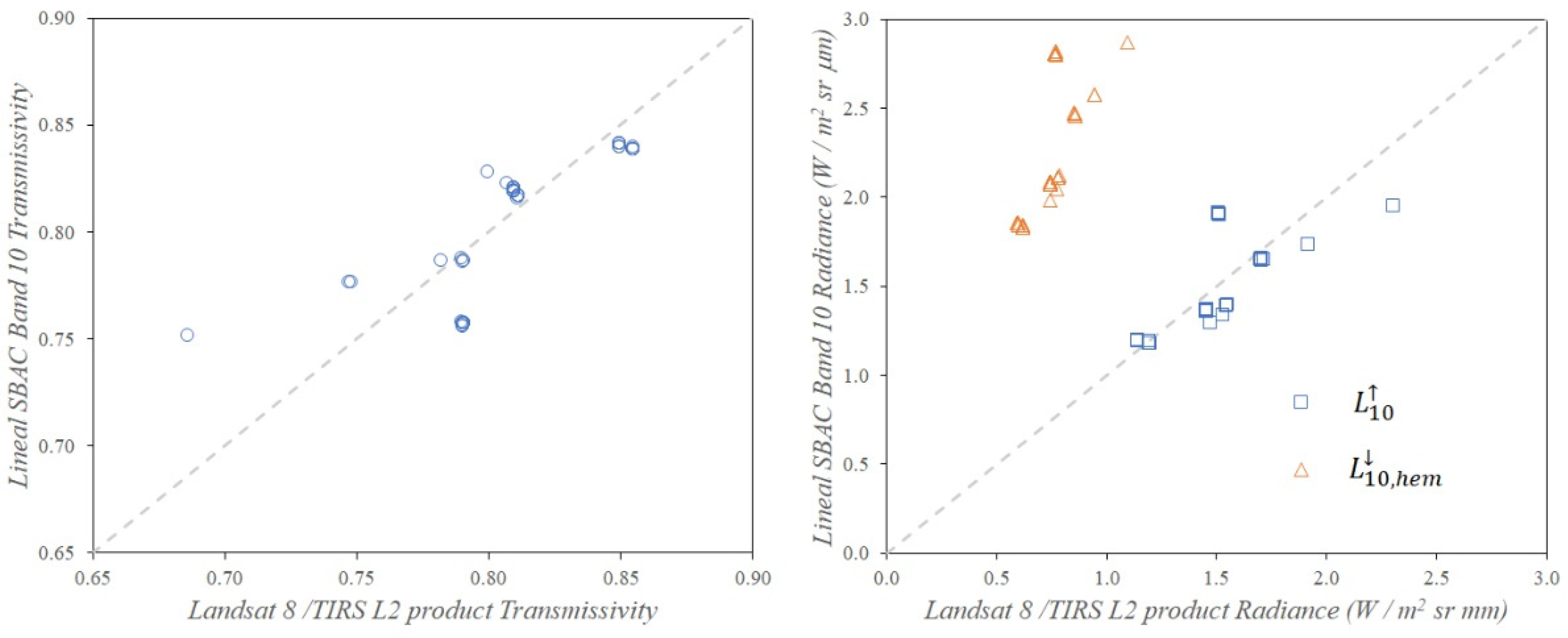
2.1.2. The Single Band Atmospheric Correction (SBAC)

Recent efforts in LST retrieval from Landsat have led to new methodologies to build up pixel-by-pixel maps of atmospheric correction parameters. Single Band Atmospheric Correction (SBAC, [30]) is a new tool based on NCEP profiles and MODTRAN v5.2 [35,36] radiative transfer code. The SBAC tool has been successfully applied before to Landsat 7/ETM+ [29] and Envisat/AATSR [37]. In this work, SBAC is adapted to channels 10 and 11 of L8/TIRS. SBAC interpolates the atmospheric correction parameters, taking into account the time, location, and elevation of a given pixel, no matter what the spatial resolution is. SBAC builds up two tridimensional grids, closest in time prior to and after the sensor overpass, covering the full scene and 13 different elevation levels from 0 m to 5000 m a.s.l. In each node (time-latitude-longitude) the atmospheric profile used as input in MODTRAN v5.2 is modified to be adapted to the pixel elevation, following the procedure described in [30].

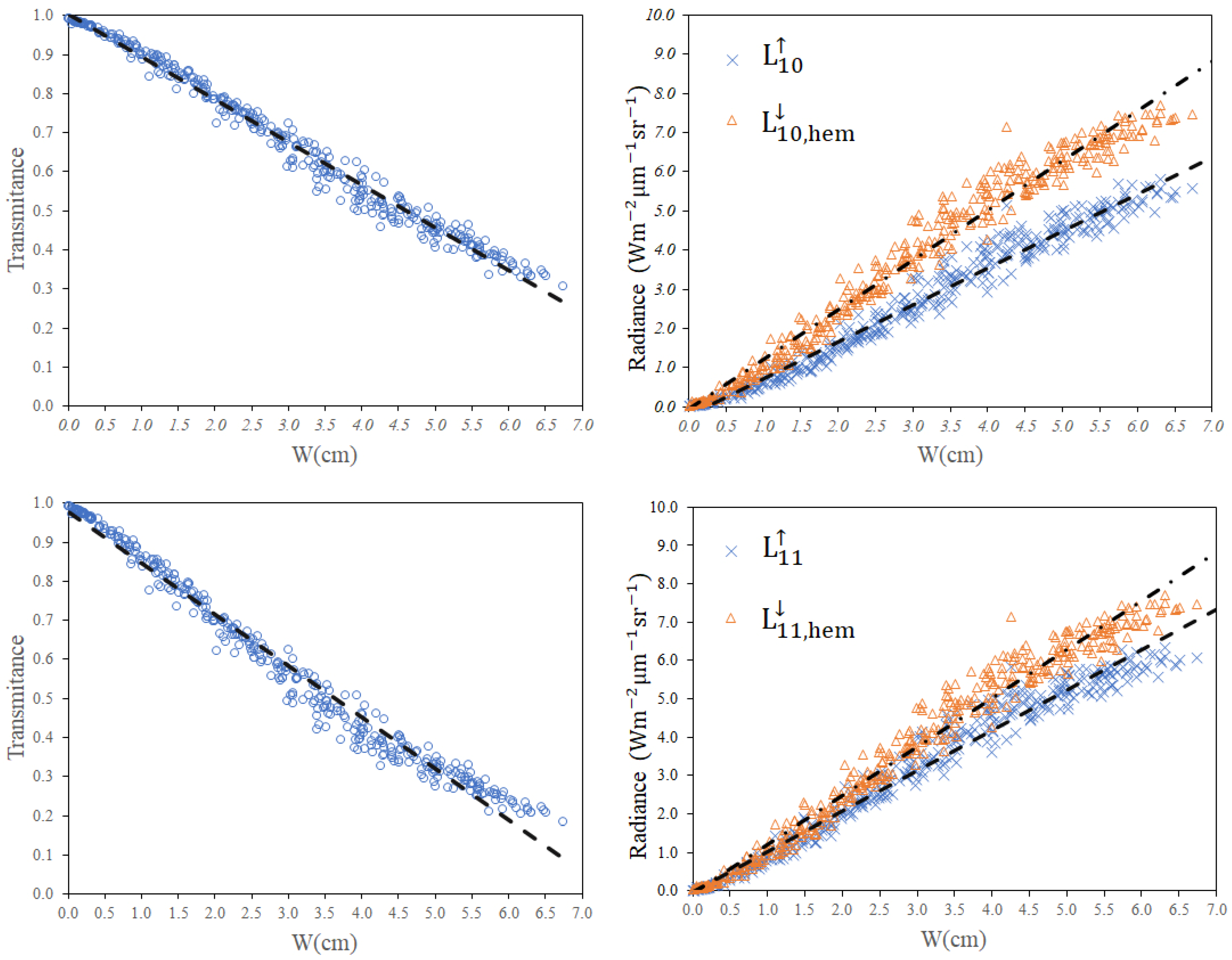
2.1.3. Linear Approach for SBAC (L-SBAC)

Time consumption and the complexity in the calculation procedure of the SBAC methodology render its use inefficient when near Real-Time product is needed. To increase the effectiveness of SBAC, a linear regression between the atmospheric correction parameters and the water vapor content (w) is introduced in the L-SBAC approach. The Cloudless Land Atmospheric Radiosonde dataset (CLAR, [38]) was used to derive these statistical regressions. The CLAR database was set with the aim of simulating radiometric measurements from satellite-borne sensors in the thermal infrared. This database contains 382 radiosounding profiles acquired over land that homogenously cover water vapor content from 0 to 5 cm. Figure 1 plots the results obtained for L8/TIRS bands, and a summary of the coefficients for the linear regressions is included in Table 1.

2.1.4. Jiménez-Muñoz Split-Window Algorithm

Jiménez-Muñoz et al. [33] proposed a Split-Window algorithm (SW_JM) based on the mathematical structure originally introduced by [39,40,41]. The coefficients needed were obtained from statistical fits performed over simulated data from atmospheric profile datasets used as inputs to the MODTRAN radiative transfer code. Jimenez-Muñoz et al. [33] used the Global Atmospheric Profiles from Reanalysis Information (GAPRI) as inputs. This database contains 4715 atmospheric profiles selected over land, covering tropical, midlatitude, subartic, and artic weather conditions. For further details on this SW_JM algorithm, see [34]. The algorithm can be written as follows:
T = T 10 + 1.378 ( T 10 T 11 ) + 0.183 ( T 10 T 11 ) 2 0.268 + ( 54.30 2.238 w ) ( 1 ε ) ( 16.40 w 129.20 ) Δ ε
where ε and Δε represent the mean and difference emissivity values for L8/TIRS bands 10 and 11, respectively.

2.1.5. Du Split-Window Algorithm

Du et al. [42] proposed a Split-Window approach (SW_Du) based on the generalized Split-Window algorithm of [43], which has no explicit dependence on water vapor content:
T = 0.41165 + ( 1.00522 + 0.14543   1 ε ε 0.27297   Δ ε ε 2 ) T 10 + T 11 2 + ( 4.06655 6.92512 1 ε ε 18.27461 Δ ε ε 2 ) T 10 T 11 2 + 0.24468 ( T 10 T 11 ) 2
The coefficients in Equation (7) were obtained by [42] for the whole range of values of w from 0 to 6.3 cm.

2.1.6. Split-Window Based on CLAR Database

A new Split-Window algorithm (SW_CLAR) is proposed in this work, following the typical structure of SW algorithms in the literature [33,40,41] and redefining the coefficients by using the CLAR database [38]. This database contains 382 radiosounding profiles over land, with nearly uniform distribution of precipitable water between 0.02 and 5.5 cm. The sondes are distributed in three latitude ranges, with around 40% of radiosoundings placed at low latitudes (0°–30°), another 40% at middle latitudes (30°–60°), and 20% at high latitudes (> 60°). The temperature of the first layer of the radiosoundings (T0) ranges from −20 °C to 40 °C. The setup of the simulations performed considers the simulated ground T as following a Gaussian distribution: T0 − 6, T0 − 2, T0 + 1, T0 + 3, T0 + 5, T0 + 8, and T0 + 12. Radiative transfer calculations are performed with the MODTRAN 5 code for two viewing angles; in this case, the nadir and the Gaussian angle 11.6° [44], sufficient to account for the 15° field of view of L8. The resulting radiance spectra are convoluted with the response filter functions of L8/TIRS bands 10 and 11, and coefficients in Equation (8) were derived:
T = T 10 + 0.357 ( T 10 T 11 ) + 1.867 ( T 10 T 11 ) 2 + 0.148 + ( 47.72 + 4.08   w   1.34   w 2 ) ( 1 ε ) + ( 27.3   w 139.3 ) Δ ε
Beyond the difference in the number of thermal bands used by the different algorithms, there are some common features, and also differences, between them. For instance, the three SW algorithms adopt a second-order polynomial for the temperature difference between bands, although with different coefficients. The SC_JM algorithm also adopts a quadratic relation with the brightness temperatures, whereas the SBAC and L-SBAC models follow the radiative transfer equation. Another similarity between models is that they all depend on surface emissivity. While emissivity information for a single band (10 or 11) is required for SC algorithms, SW approaches need the emissivity from both spectral ranges to run. The main differentiating feature between the algorithms is the way atmospheric correction is conducted. All the algorithms, except SW_Du, need the water vapor content as an input, but the way this is estimated and implemented varies. SW_JM considers a linear dependence with w, whereas SC_JM and SW_CLAR opt for a second-order polynomial. The strength of SBAC is its capability to account for the spatio-temporal and orography variability within a scene, although its operational application may be computationally demanding. A shortcut is introduced with L-SBAC through a linear approximation with w data. In summary, the six LST algorithms selected for this study feature a variety of approaches, some of them well-known and widely used (SC_JM, SW_JM or SW_Du) and others more recently introduced (SBAC), in addition to the new L-SBAC and SW_CLAR also explored in this work.

2.2. Landsat 8 LST L2 Product

As part of the Level-2 Science Products (L2SP), the USGS has released an operational LST product (L8_ST) derived from L8 Collection 2 Level-1 data [45]. This product is also based on the radiative transfer equation applied to L8/TIRS band 10 radiances. North American Regional Reanalysis (NARR) data are used to characterize the atmosphere in this case, and MODTRAN code is used to perform the radiative transfer calculations. Atmospheric data are interpolated in time, elevation, and pixel location to provide per-pixel atmospheric compensation values. The emissivity correction for this product is based on data from the ASTER Global Emissivity Dataset (ASTER-GED, [46]), temporally adjusted to the target Landsat scene through ASTER Normalized Difference Vegetation Index (ASTER NDVI) information.
L8_ST product is available with a 16 day period through the Earth Explorer website (https://earthexplorer.usgs.gov/, accessed on 1 March 2022). In addition to the LST information, the operational product provides all the variables involved in the atmospheric compensation process, including emissivity in band 10, atmospheric transmittance, and upwelling and downwelling radiances [22]. Note that L8_ST products are available approximately 15–17 days after acquisition and this is a concern for near Real-Time applications.

2.3. Emissivity and Water Vapor Content Inputs

2.3.1. Emissivity Estimation

Emissivity values for natural surfaces are usually estimated by weighting the vegetated and soil portions of every pixel. The NDVI has been traditionally used as an input to quantify the vegetation cover fraction (Pv) for remote sensing. Based on the results of a theoretical and experimental study, Valor and Caselles [47,48] proposed the following approach to estimate the emissivity of a natural surface:
ε i = ε i , v P v + ε i , s ( 1 P v ) ( 1 1.74 P v ) + 1.7372 P v ( 1 P v )
where εi,v and εi,s are the emissivity assigned to pure samples of full vegetation cover and bare soil, respectively. Hulley and Hook [49] calculated these values for ASTER bands using 58 soil spectra from the ASTER Spectral Library (ASL, [50]), covering all soil taxonomy, in addition to the conifer spectra measurement made by Johns Hopkins University (JHU). Applying this same procedure, adapted now to the thermal channels of L8/TIRS, values of 0.971 and 0.994 were obtained for bare soil and fully vegetated pixels, respectively, for band 10, and 0.977 and 0.995 for band 11.
According to [47,48], Pv in Equation (3) is obtained from the NDVI ( N D V I = ( ρ N I R ρ R ) / ( ρ N I R + ρ R ) ), ρNIR and ρR being reflectances in the near-infrared and red bands, respectively:
P v = ( 1 N D V I N D V I s ) ( 1 N D V I N D V I s ) + K ( 1 N D V I N D V I v ) ,
where the subindices s and v stand for pure bare soil and full vegetated pixels, respectively. K is defined as the quotient of the contrasts between infrared and red reflectance in fully vegetated surfaces and bare soil surfaces K = ( ρ i r v ρ r v ) / ( ρ i r s ρ r s ) .
The correct choice of these two pure sites is critical for accurate emissivity estimation. In this work, an analysis of the evolution of the NDVI during typical years in different crops is conducted. Alfalfa, corn, vineyard, and wheat fields are selected, as well as bare soil parcels. A total of 3326 measurements from 2014 to 2018 in crop fields of Albacete (Spain) are used. Figure 2 shows the temporal evolution of the mean NDVI values for the selected land covers, accessible from the WebGIS platform (www.spiderwebgis.org, accessed on 10 February 2022).
Alfalfa, corn, and wheat are crops with a capacity to reach full covered conditions, showing mean values of maximum NDVI of 0.86 ± 0.03, 0.820 ± 0.012, and 0.86 ± 0.03, respectively. A threshold of 0.85 in NDVI is set in this work for considering a pixel as fully vegetated. Regarding bare soil, a threshold of 0.15 was established. These match with the previous studies that assume values of NDVI of 0.93 and 0.14 for full vegetated and bare soil conditions, respectively [51,52].

2.3.2. Spatially Distributed Total Column Water Vapor Content

All the algorithms above share the need for an estimation of the total column water vapor content (w) for every single pixel in the image (except SW_Du). However, there are no operational products available offering this variable with sufficient spatio-temporal concurrence and with L8/TIRS overpass. In the present work, we introduce a methodology inspired by the SBAC interpolation method [30] to obtain w. The main steps can be summarized as follows:
  • Data from the NCEP global tropospheric analyses product are used. This product provides atmospheric profiles of temperature, air humidity, and geopotential height in several constant pressure levels every 6 h.
  • The SBAC interpolation method defines a tri-dimensional grid with nodes latitude-longitude and thirteen height levels from 0 to 5000 m above the sea. Every node/level coordinate is filled with a calculated W from an atmospheric profile above the determinate level, temporally interpolated between the two closest in time products prior to and after the sensor overpass.
  • Once a pixel is selected, the eighteen closest nodes-levels are activated (nine above and nine below of selected pixels) based on the corresponding latitude, longitude, and height above sea level.
  • Weighted spatial interpolation, with the distance square as a basis, is used to obtain W only in the level above and below the desired pixel. Finally, a linear interpolation between two levels yields the w value for the selected pixel.
This methodology for obtaining w allows for the specialization of this variable to any resolution, time, and scene, wrapping to the elevation of the terrain.

2.4. Evaluation Statistics

To evaluate the accuracy of the different models, the satellite-derived LSTs were compared to the ground measurements (Tg), used as ground-truth reference. Two sets of statistical parameters were used for the assessment. First, some statistics focused on the result uncertainty, such as the biased estimator (Bias), the Standard Deviation (σ), the Root Mean Square Error (RMSE), and the Mean Absolute Error (MAE). A second set of statistics was implemented to evaluate the efficiency and scatter, the slope and interception of the linear adjustments between estimates and ground measurements of LST, and the regression coefficient (R2).

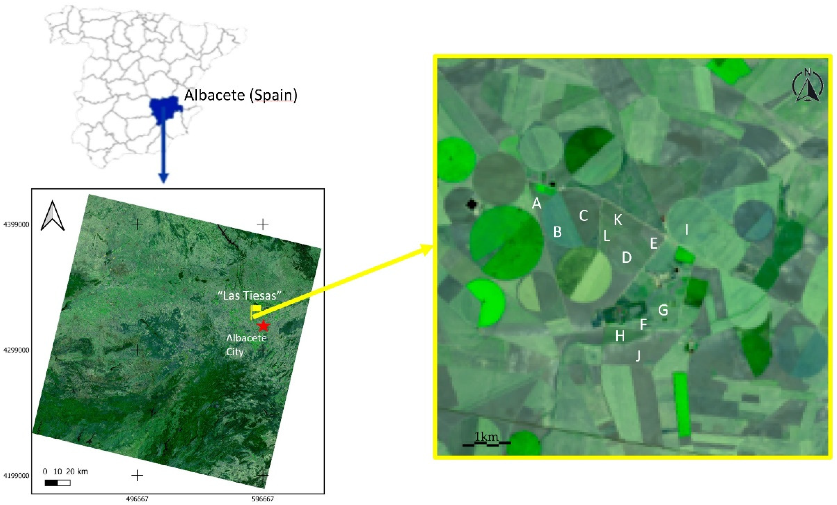
3. Study Site and Measurements

The study site for this work is a semiarid agricultural area of southeastern Spain located in the “Las Tiesas” experimental farm (39.03035N, 2.060W). This is a high-contrast flat cropland area with an average altitude of 700 m above sea level close to Albacete, frequently used as an experimental site in the framework of international campaigns involving ground, airborne, and satellite sensors [53,54,55,56,57]. The “Las Tiesas” site falls within the overlapped area between Landsat tiles WRS 200/33 and WRS 199/33 (path/row). This guarantees one image per week will cover our study site.
Ground LST measurements were taken concurrently with L8/TIRS overpasses during the summer seasons of 2018–2019 in a set of crop fields selected to cover a variety of vegetation cover conditions: barley, vineyard, corn, garlic, poppy, wheat, onion, and almond orchard. An overview of the study area and the crop fields is shown in Figure 3. The extension of all selected plots is >10 ha (except for the vineyard with ~5 ha), which guarantees a minimum of 3 × 3 Landsat pixels within each plot. The temperatures were measured using three Apogee MI-210 hand-held infrared radiometers (IRTs). These radiometers have a broad thermal band (8–14 µm) with an accuracy of ±0.3 K and a 22° field of view. All radiometers were calibrated against a black body (Landcal-P80, also calibrated in an international blackbody inter-comparison field campaign, [58]) before and after every campaign. In the sparse crops (vineyard and almond trees), special care was taken in the measurements, averaging soil and canopy temperatures so as to obtain representative values of the target LST.
A total set of 11 L8/TIRS scenes was selected for this work. All are cloud-free images with available ground data for the evaluation. Collection 2 Level-1 and Level-2 L8 products were downloaded and processed, with a pixel size of 30 m. Table 2 lists the ground data available for each date/scene. All of these ground measurements were taken under cloudless sky conditions. Ground transects were conducted by carrying the radiometer back and forth, pointing to the surface in a nadir view, and at a height of 1–1.5 m above the ground. The temperature was registered at a rate of 5–10 samples/min, covering 30–50 m/min, and a total area of several hectares in each plot. Ten-minute average values centered on the satellite overpass times were calculated. Ground temperatures were corrected from atmospheric and emissivity effects. For this, downwelling sky emission was registered for each radiometer and date [59]. Emissivity data were obtained by applying the Temperature-Emissivity-Separation (TES) methodology [46,60] to the on-site measurements using a CIMEL CE312-2 multispectral thermal infrared radiometer [61]. Broadband emissivity values (8–13 µm) were used in this case.

4. Results

4.1. Ground Measurements and Satellite Brightness Temperatures

The averaged 10 min ground LST measurements (Tg) centered in the L8 overpass were measured for all items presented in Table 2. The uncertainty in ground temperature corresponding to the standard deviation of these measurements ranged from ±0.5 K to ±1.2 K, accounting for the temporal (10 min) and spatial (several hectares) variability of the LST at the test site. Emissivity values for both band 10 and band 11 were obtained following the methodology in Section 2.3.1, using NDVI values obtained using reflectance data from the L8/Operational Land Imager’s (OLI) red and infrared data (bands 4 and 5, respectively) provided in the Level-1 product. Note that Level-1 data must be used at this step to achieve near Real-Time LST estimation. Total water vapor content (w) for each site/date was derived following the procedure described in Section 2.3.2, yielding values between 1.5 cm and 2.3 cm. Mean emissivity and brightness temperature values for the 3 × 3 pixels centered in the exact location of the ground transects were extracted from the images to guarantee the spatial matching between ground and satellite LST data. Table 3 lists these average values, together with their standard deviation, for the 3 × 3 pixels centered in the coordinates of each site (#) labeled in Table 2. Note that the same emissivity values were used for all the algorithms tested to focus and constrain their differences in terms of atmospheric correction.

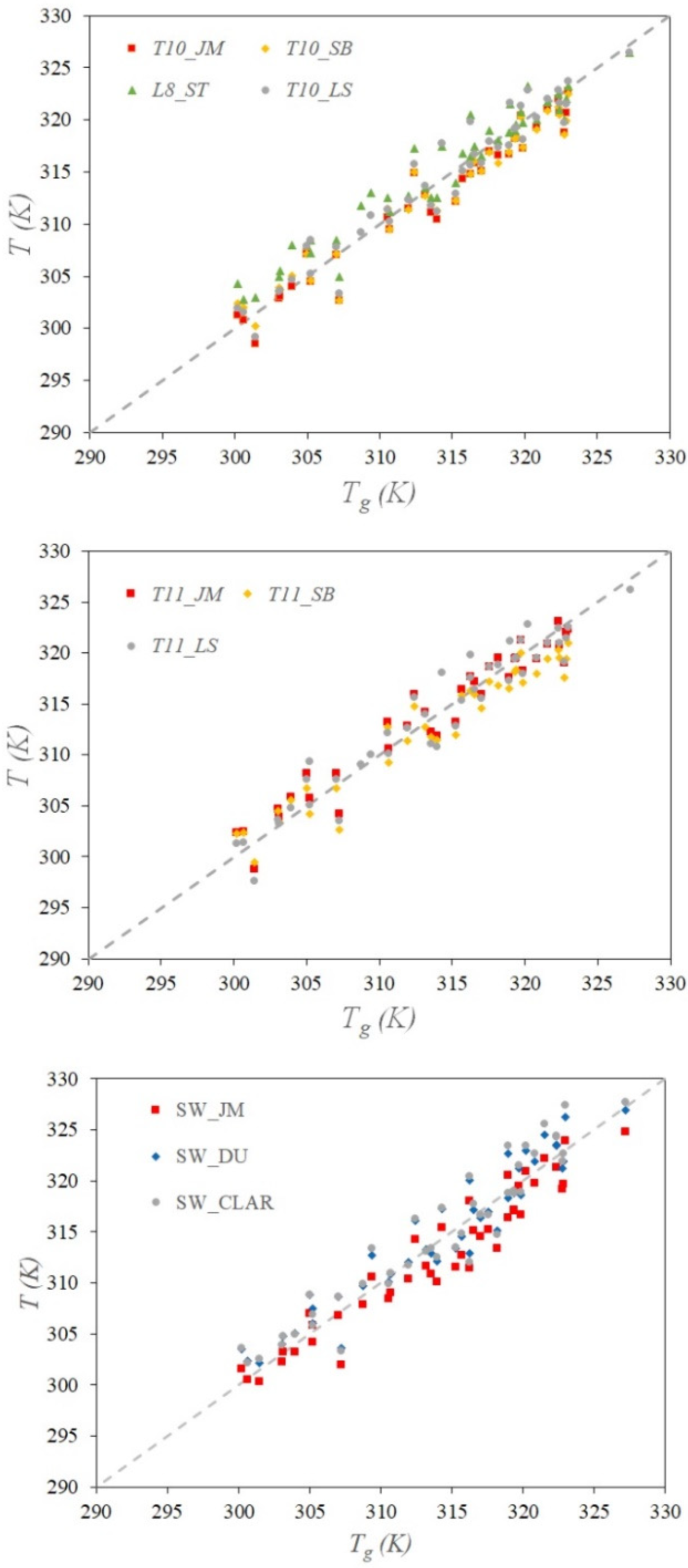
4.2. Single-Channel LST

All described SC algorithms were applied to the set of 11 images available for this work. Figure 4 shows an example of LST maps corresponding to date 24 July 2018. These images illustrate the large variability in LST within the study site, with no significant differences between algorithms at first sight. Plots in Figure 5 and statistics in Table 4 show the assessment of the SC algorithms described in Section 2.1 in terms of LST retrieval, using the ground measurements as a reference. This intercomparison involves the traditional [33] algorithm (T10_JM, Equation (4)) and the [18] adaptation to band 11 (T11_JM, Equation (5)), the results being obtained by using the radiative transfer equation together with atmospheric correction parameters obtained from the SBAC tool (T10_SB and T11_SB), or the linear approximation (Table 1, T10_LS and T11_LS). Finally, the operational L8/TIRS LST product (L8_ST) is included in the analysis. A more detailed analysis of the results, filtering by crop type, is shown in Table 5. Cereals (wheat and barley) are presented together due to the growing similarity between both crops. Stubble and onion were not included in this per-crop analysis since a single dataset for each was available.
Overall, the results obtained from all the SC algorithms were equivalent with no significant differences between them, except for the L8_ST product. The estimation error in all cases was between ±1.8 K and ±2.0 K, independent of the band used. If we focus on the systematic deviation of the models, Linear SBAC yields practically no bias with a small overestimation of 0.1 K (0.2 K) for band 10 (11). The SBAC and JM methodologies reproduce a similar underestimation of around −0.6 K using bands 10 and 11, except for the case of T11_JM (Equation (5)), in which an overestimation of 0.6 K is observed. Better results were obtained using band 10 versus band 11. Mean Average Error (MAE) values of ±1.4 K for T10_LS and ±1.5 K for both T10_JM and T10_SB were observed against MAE values up to ±1.7 K for T11_JM and T11_SB.
Regarding the operational L8_ST product, an overestimation of 1.0 K is obtained, although with a standard deviation of ±1.9 K, resulting in a MAE of ±1.7 K. This systematic deviation in the LST provided by the USGS operational product needs further analysis, provided in a section below.

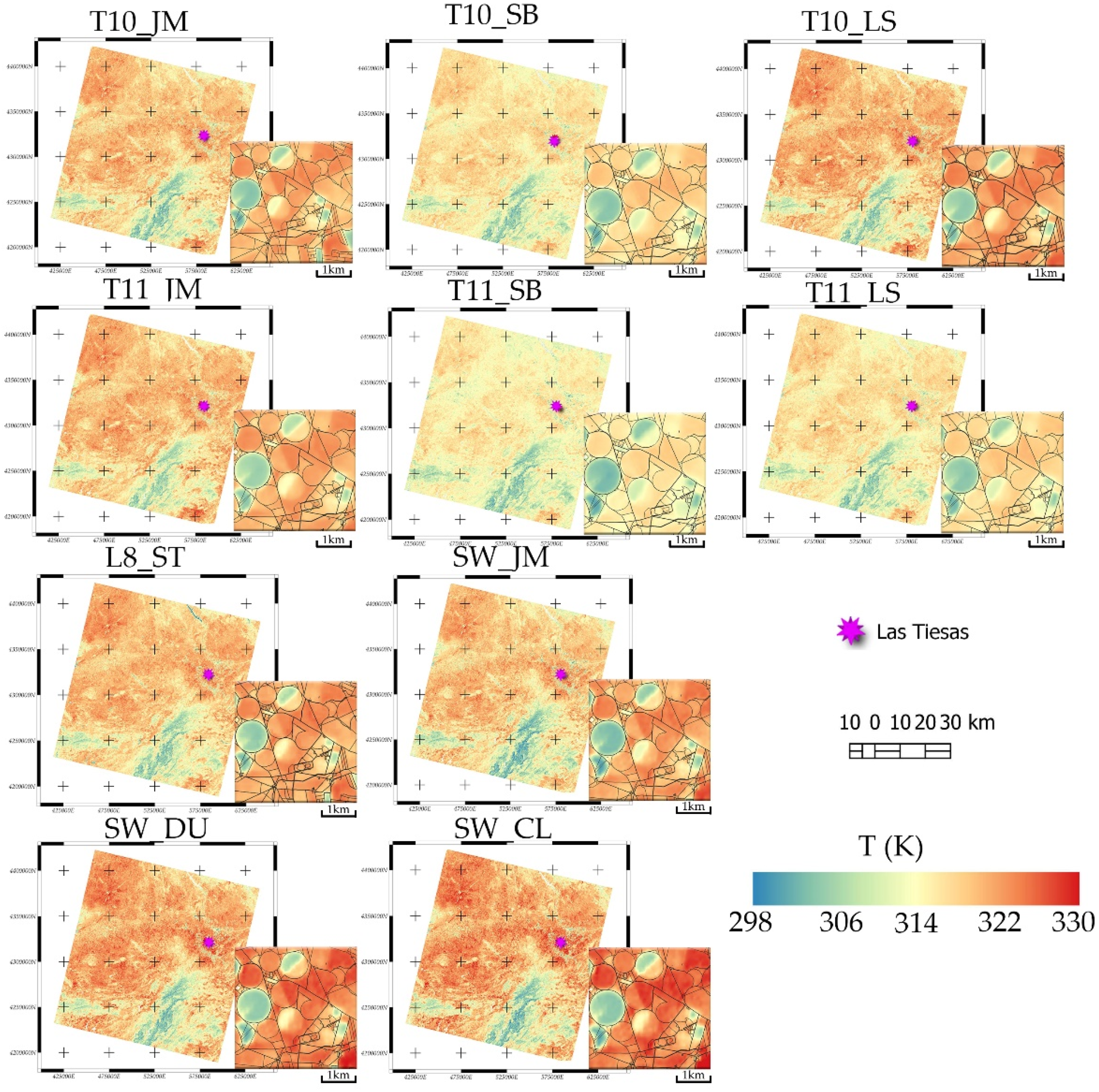
4.3. Split-Window LST

Focusing now on the results from the Split-Window algorithms, Figure 5 also plots the intercomparison between the surface temperatures obtained with SW_JM [33], SW_DU [42], and SW_CLAR, the latter being described in Section 2.1.6 and based on the methodology by [38].
The main results for the SW algorithms are summarized in Table 4. The three approaches perform very similarly, with a common RMSE of ±2.0 K. An underestimation of −1.2 K is observed with the SW_JM algorithm, whereas SW_DU and SW_CLAR overestimate the ground-measured LSTs by 0.7 and 0.9 K, respectively. Results are in good agreement with recently published works [62], noting the good performance of the SW algorithms and evidencing the slight advantage of SW_DU with respect the other algorithms, since it does not need any atmospheric input.
Overall, estimation errors from using SW formulations do not differ significantly to those obtained from applying SC algorithms in terms of accuracy, although a slight increase in the BIAS is noticed.

5. Discussions

The primary aim of this work is the assessment of the performance of the LST estimates from L8 under the specific conditions of our semiarid site, and focusing on agricultural targets for the further implication of this parameter in water management or irrigation scheduling tasks. This study does not intend to be a pure intercomparison of algorithms, as that would require a larger variety of atmospheric conditions and even more homogeneous surfaces. Nevertheless, under this premise, the results of SC algorithms from this study are in good agreement with (or even improve upon) those published in recent literature [20,63]. These authors tested different SC algorithms applied to L8, and reported mean BIAS errors of −1 K and a RMSE of ±2–3 K, when compared with in situ data from seven to twelve SURFRAD and ARM stations measuring grassland and cropland surfaces. Further, similar validation results were reported by Wang et al. [64] and Ermida et al. [65] using a proposed SC algorithm framework for producing global long time-series of Landsat LST retrievals on the Google Earth Engine (GEE) cloud computing platform. Mean BIAS values within 0.6 K and RMSE of ±2 K were obtained by these authors when compared with in situ LST data from different SURFRAD stations. The good results also reported when using band 11 prove the improvement in this spectral band implemented in the released L8 Collection 2. Differences in the LST derived from both band 10 and 11, separately, can be then used to test the reliability and feasibility of a model, assuming that the surface temperature is independent of the spectral range considered for its estimation. Table 6 shows the statistics of the differences between T10T11 from the different SC methodologies studied in this work.
Note that the SBAC methodology and its linear approach (L-SBAC) are less sensitive to the bands used (10 or 11), yielding negligible BIAS and a low MAE (±0.5 K). However, the JM methodology shows a stronger dependence, with a mean difference of 1.2 K instead.
Regarding the operational USGS LST product, this work contributes to filling the gap in the existing literature regarding its performance under the conditions of semiarid agroecosystems. To better understand the sources of bias of the L8_ST product in our site, shown above, we can investigate the uncertainties in both the atmospheric parameters and emissivity values implemented in the USGS L8_ST product for the correction of the brightness temperatures. The plots in Figure 6 show the comparison between the atmospheric correction parameters obtained through the linear SBAC approach proposed (Table 1) against those provided by the L8 L2SP product. Results from both methods are very similar in terms of atmospheric transmissivity and upwelling radiance, with minor differences that may be a consequence of the atmospheric profiles used as inputs. On the contrary, significant differences appear in the values for downward hemispherical radiance, with values that almost triple those provided by the L8 L2SP product. Nevertheless, a sensitivity analysis of this parameter shows that strong variations of this parameter do not have considerable effects on LST retrieval; as such, the impact on LST due to this uncertainty is expected to be lower than 0.2 K. Recalculated L8_ST, implementing downward hemispherical radiance values obtained with Linear SBAC, reduces the overestimation to 0.9 K and the MAE to ±1.6 K, although this reduction is minor and the systematic differences in LST still remain.
The emissivity values for band 10 [46] are also provided as one of the L2SP products. Figure 7 shows the comparison between our self-derived emissivity values, retrieved following the methodology described in Section 2.3.1, against those provided by the L8 L2SP product for the study plots.
The emissivity values provided by the L8 L2SP product are significantly lower than our estimations. This discrepancy could be a consequence of an improper land use classification or vegetation content estimation. It is well known that minor differences in emissivity may lead to significant deviations in LST. A sensitivity analysis was carried out to quantify the effect of emissivity deviations in the LST retrieval. A discrepancy of 0.5% in emissivity yields an LST uncertainty of ±0.5 K for L8_ST and ± 0.4 K for T10_LS. However, if the discrepancy increases up to 2%, as reported above for the emissivity values in the L8_ST product, deviation in LST reaches ±2.0 K for L8_ST and ± 1.8 K for T10_LS. Therefore, this underestimation in the emissivity values justifies the overestimation in LST values of the L8_ST product shown above. A recalculation of these LST values using our emissivity estimates reduces the underestimation of the L8_ST product to 0.2 K, resulting in a final MAE of ±1.5 K. This necessity for a tuning in the LSE correction of the operational L8 LST product was previously pointed out by Duan et al. [63].
Finally, the results using the simplified and faster version of SBAC are promising. L-SBAC could be then implemented to generate time series of LST images from L8 in semiarid agroecosystems at a near Real-Time rate, saving computational resources. The performance of L-SBAC must be further evaluated under a larger variety of environmental and surface conditions in future works.

6. Conclusions

This work focuses on the assessment of LST retrieval from L8/TIRS under the conditions of a heterogeneous cropland area in a semiarid region, where temperatures during a typical spring-summer growing season range between 295 K and 325 K for irrigated covers and bare soil surfaces, respectively, at the satellite overpass time. The Barrax test site in Spain provided a unique opportunity for this experiment of LST validation and intercomparison of algorithms, using ground transects of LST covering a variety of surface conditions concentrated in a few square kilometers within a Landsat scene. This ground dataset itself is a major contribution of this work, since ground transects of LST under these conditions are quite rare in the literature. Performance is very similar for the total of seven LST algorithms tested: four Single-Channel, including the USGS operational product, and three Split-Window. Estimation errors were below ±2.0 K in all cases, with systematic deviations mostly within 1.0 K. Nevertheless, slightly better accuracy was obtained with SC compared to SW algorithms, especially with those using band 10, although the good performance of band 11 is also noticeable.
Results using the linear approach of the SBAC methodology (L-SBAC) for LST retrieval from L8 are promising in our region, based on the good accuracy observed, with average values of BIAS = +0.2 K and RMSE = ±1.8 K for the full dataset, and no significant differences between crop types. Furthermore, L-SBAC significantly reduces the computational resources, and thus the time frame, needed to generate and provide operational LST maps from L8 Level 1 data. L-SBAC will be particularly attractive for those applications when near Real-Time LST data are needed, since an LST product could be ready within 2–3 h after acquisition. Water management or irrigation scheduling tasks could benefit from prompt LST information, and this becomes critical in agroecosystems with limited water resources.
This study also contributes to the assessment of the USGS L8_ST product in the Barrax test site. Results show this operational product performs well in our cropland area, and the systematic overestimation of 1.0 K observed can be justified by the erroneous assignment of emissivity values for the targets. These findings are in agreement with the few results reported in the literature and contribute to taking further actions for the tuning of the L8_ST product.

Author Contributions

Conceptualization, J.M.G. and J.M.S.; methodology, J.M.G., J.M.S., J.V. and J.G.-P.; validation, J.M.G., J.M.S. and J.G.-P.; formal analysis, J.M.G. and J.M.S.; investigation, J.M.G., J.M.S., J.G.-P. and A.C.; data curation, J.M.S., J.M.G. and J.V.; writing—original draft preparation, J.M.G. and J.M.S.; writing—review and editing, V.G.-S. and J.G.-P.; project administration, J.M.S., J.G.-P. and A.C.; funding acquisition, J.M.S., J.G.-P. and A.C. All authors have read and agreed to the published version of the manuscript.

Funding

This work was funded by the Spanish Economy and Competitiveness Ministry (projects PID2020-113498RB-C21 and PID2020-118797RB-I00), the Education, Culture and Sports Council (JCCM, Spain) (ANIATEL project SBPLY/17/180501/000357). Both together with FEDER funds. Financial support of the European Commission (NEXUS project, grant number 101003632) is also acknowledged.

Data Availability Statement

The data presented in this study are available on request from the corresponding author.

Acknowledgments

The authors would like to acknowledge the logistic support and access to the facilities of the ITAP-FUNDESCAM in Las Tiesas experimental farm during the field campaigns.

Conflicts of Interest

The authors declare no conflict of interest.

References

  1. Anderson, M.C.; Allen, R.G.; Morse, A.; Kustas, W.P. Use of Landsat thermal imagery in monitoring evapotranspiration and managing water resources. Remote Sens. Environ. 2012, 122, 50–65. [Google Scholar] [CrossRef]
  2. Trigo, I.F.; Boussetta, P.S.; Viterbo, G.; Balsamo, A.; Sandu, I. Comparison of model land skintemperature with remotely sensedestimates and assessment of surface-atmosphere coupling. J. Geophys. Res. Atmos. 2015, 120, 12096–12111. [Google Scholar] [CrossRef] [Green Version]
  3. Fisher, J.B.; Melton, F.; Middleton, E.; Hain, C.; Anderson, M.; Allen, R.; McCabe, M.F.; Hook, S.; Baldocchi, D.; Townsend, P.A.; et al. The future ofevapotranspiration: Globalrequirements for ecosystemfunctioning, carbon and climatefeedbacks, agricultural management, and water resources. Water Resour. Res. 2017, 53, 2618–2626. [Google Scholar] [CrossRef]
  4. Guillevic, P.; Göttsche, F.; Nickeson, J.; Hulley, G.; Ghent, D.; Yu, Y.; Trigo, I.; Hook, S.; Sobrino, J.A.; Remedios, J.; et al. Land surface temperature product validation best practice protocol version 1.1. Best Pract. Satell.-Deriv. Land Prod. Valid. 2018. Available online: https://lpvs.gsfc.nasa.gov/PDF/CEOS_LST_PROTOCOL_Feb2018_v1.1.0_light.pdf (accessed on 15 January 2022).
  5. Su, H.; McCabe, M.; Wood, E.F.; Su, Z.; Prueger, J. Modeling evapotranspiration during SMACEX: Comparing two approaches for local-and regional-scale prediction. J. Hydrometeorol. 2005, 6, 910–922. [Google Scholar] [CrossRef]
  6. Kalma, J.D.; McVicar, T.R.; McCabe, M.F. Estimating Land Surface Evaporation: A Review of Methods Using Remotely Sensed Surface Temperature Data. Surv. Geophys. 2008, 29, 421–469. [Google Scholar] [CrossRef]
  7. Sánchez, J.M.; Scavone, G.; Caselles, V.; Valor, E.; Copertino, V.A.; Telesca, V. Monitoring daily evapotranspiration at a regional scale from Landsat-TM and ETM+ data: Application to the Basilicata region. J. Hydrol. 2008, 351, 58–70. [Google Scholar] [CrossRef]
  8. Kustas, W.P.; Alfieri, J.G.; Nieto, H.; Wilson, T.G.; Gao, F.; Anderson, M.C. Utility of the two-source energy balance (TSEB) model in vine and interrow flux partitioning over the growing season. Irrig. Sci. 2019, 37, 375–388. [Google Scholar] [CrossRef]
  9. Food and Agriculture Organization of United Nations. Innovation in Family Farming; The State of Food and Agriculture: Rome, Italy, 2014; E-ISBN 978-92-5-108537-0. [Google Scholar]
  10. Tilman, D.; Cassman, K.G.; Matson, P.A.; Naylor, R.; Polasky, S. Agricultural sustainability and intensive production practices. Nature 2002, 418, 671–677. [Google Scholar] [CrossRef]
  11. Garnett, T.; Appleby, M.C.; Balmford, A.; Bateman, I.J.; Benton, T.G.; Bloomer, P.; Burlingame, B.; Dawkins, M.; Dolan, L.; Fraser, D.; et al. Sustainable Intensification in Agriculture: Premises and Policies. Sci. Mag. 2013, 341, 33–34. [Google Scholar] [CrossRef]
  12. Wulder, M.A.; White, J.C.; Loveland, T.R.; Woodcock, C.E.; Belward, A.S.; Cohen, W.B.; Fosnight, E.A.; Shaw, J.; Masek, J.G.; Roy, D.P. The global Landsat archive: Status, consolidation, and direction. Remote Sens. Environ. 2016, 185, 271–283. [Google Scholar] [CrossRef] [Green Version]
  13. Dwyer, J.L.; Roy, D.P.; Sauer, B.; Jenkerson, C.B.; Zhang, H.K.; Lymburner, L. Analysis Ready Data: Enabling Analysis of the Landsat Archive. Remote Sens. 2018, 10, 1363. [Google Scholar] [CrossRef]
  14. Irons, J.R.; Dwyer, J.L.; Barsi, J.A. The next landsat satellite: The landsat data continuity mission. Remote Sens. Environ. 2012, 122, 11–21. [Google Scholar] [CrossRef] [Green Version]
  15. Montanaro, M.; Barsi, J.; Lunsford, A.; Rohrbach, S.; Markham, B. Performance of the Thermal Infrared Sensor on-board Landsat 8 over the first year on-orbit. In Proceedings of the Earth Observing Systems XIX, San Diego, CA, USA, 17–21 August 2014; p. 921817. [Google Scholar] [CrossRef]
  16. Barsi, J.A.; Lee, K.; Kvaran, G.; Markham, B.L.; Pedelty, J.A. The Spectral Response of the Landsat-8 Operational Land Imager. Remote Sens. 2014, 6, 10232–10251. [Google Scholar] [CrossRef] [Green Version]
  17. Gerace, A.; Montanaro, M. Derivation and validation of the stray light correction algorithm for the thermal infrared sensor onboard landsat 8. Remote Sens. Environ. 2017, 191, 246–257. [Google Scholar] [CrossRef]
  18. Guo, J.; Ren, H.; Zheng, Y.; Lu, S.; Dong, J. Evaluation of Land Surface Temperature Retrieval from Landsat 8/TIRS Images before and after Stray Light Correction Using the SURFRAD Dataset. Remote Sens. 2020, 12, 1023. [Google Scholar] [CrossRef] [Green Version]
  19. Niclòs, R.; Puchades, J.; Coll, C.; Barberà, M.J.; Pérez-Planells, L.; Valiente, J.A.; Sánchez, J.M. Evaluation of Landsat-8 TIRS data recalibrations and land surface temperature split-window algorithms over a homogeneous crop area with different phenological land covers. ISPRS J. Photogramm. Remote Sens. 2021, 174, 237–253. [Google Scholar] [CrossRef]
  20. Wang, M.; Zhang, Z.; Hu, T.; Liu, X. A Practical Single-Channel Algorithm for Land Surface Temperature Retrieval: Application to Landsat Series Data. J. Geophys. Res. Atmos. 2019, 124, 299–316. [Google Scholar] [CrossRef]
  21. Duan, S.-B.; Li, Z.-L.; Wang, C.; Zhang, S.; Tang, B.-H.; Leng, P.; Gao, M.-F. Land-surface temperature retrieval from Landsat 8 single-channel thermal infrared data in combination with NCEP reanalysis data and ASTER GED product. Int. J. Remote Sens. 2019, 40, 1763–1778. [Google Scholar] [CrossRef]
  22. Sayler, K. Landsat 8-9 Collection 2 Level 2 Science Product Guide. 2020. Available online: https://www.usgs.gov/media/files/landsat-8-collection-2-level-2-science-product-guide (accessed on 15 January 2022).
  23. Pérez-Planells, L.; García-Santos, V.; Caselles, V. Comparing different profiles to characterize the atmosphere for three MODIS TIR bands. Atmos. Res. 2015, 161, 108–115. [Google Scholar] [CrossRef] [Green Version]
  24. Coll, C.; Caselles, V.; Valor, E.; Niclòs, R. Comparison between different sources of atmospheric profiles for land surface temperature retrieval from single channel thermal infrared data. Remote Sens. Environ. 2012, 117, 199–210. [Google Scholar] [CrossRef]
  25. Kalnay, E.; Kanamitsu, M.; Kistler, R.; Collins, W.; Deaven, D.; Gandin, L.; Iredell, M.; Saha, S.; White, G.; Woollen, J.; et al. The NCEP/NCAR 40-year reanalysis project. Bull. Am. Meteorol. Soc. 1996, 77, 437–471. [Google Scholar] [CrossRef] [Green Version]
  26. Seemann, S.W.; Borbas, E.E.; Li, J.; Menzel, W.P.; Gumley, L.E. MODIS Atmospheric Profile Retrieval Algorithm Theoretical Basis Document. Madison, WI: Univ. Wisconsin-Madison. 2006. Available online: http://modis-atmos.gsfc.nasa.gov/reference_atbd.html (accessed on 15 January 2022).
  27. Divakarla, M.G.; Barnet, C.D.; Goldberg, M.D.; McMillin, L.M.; Maddy, E.; Wolf, W.; Zhou, L.; Liu, X. Validation of Atmospheric Infrared Sounder temperature and water vapor retrievals with matched radiosonde measurements and forecasts. J. Geophys. Res. 2006, 111, D09S15. [Google Scholar] [CrossRef] [Green Version]
  28. Barsi, J.A.; Schott, J.R.; Palluconi, F.D.; Hook, S.J. Validation of a web-based atmospheric correction tool for single thermal band instruments. In Proceedings of the Earth Observing Systems X, San Diego, CA, USA, 31 July–4 August 2005; Volume 5882, p. 58820E. [Google Scholar] [CrossRef]
  29. Coll, C.; Galve, J.M.; Sanchez, J.M.; Caselles, V. Validation of Landsat-7/ETM+ thermal-band calibration and atmospheric correction with ground-based measurement. IEEE Trans. Geosci. Remote Sens. 2010, 48, 547–555. [Google Scholar] [CrossRef]
  30. Galve, J.M.; Sánchez, J.M.; Coll, C.; Villodre, J. A New Single-Band Pixel-by-Pixel Atmospheric Correction Method to Improve the Accuracy in Remote Sensing Estimates of LST. Application to Landsat 7-ETM+. Remote Sens. 2018, 10, 826. [Google Scholar] [CrossRef] [Green Version]
  31. Li, Z.; Tang, B.; Wu, H.; Ren, H.; Yan, G.; Wan, Z.; Trigo, L.F.; Sobrino, J.A. Satellite-derived land surface temperature: Current status and perspectives. Remote Sens. Environ. 2013, 131, 14–37. [Google Scholar] [CrossRef] [Green Version]
  32. Jimenez-Munoz, J.C.; Cristobal, J.; Sobrino, J.A.; Soria, G.; Ninyerola, M.; Pons, X. Revision of the Single-Channel Algorithm for Land Surface Temperature Retrieval From Landsat Thermal-Infrared Data. IEEE Trans. Geosci. Remote Sens. 2009, 47, 339–349. [Google Scholar] [CrossRef]
  33. Jiménez-Muñoz, J.C.; Sobrino, J.A.; Skoković, D.; Mattar, C.; Cristóbal, J. Land Surface Temperature Retrieval Methods From Landsat-8 Thermal Infrared Sensor Data. IEEE Geosci. Remote Sens. Lett. 2014, 11, 1840–1843. [Google Scholar] [CrossRef]
  34. Mattar, C.; Durán-Alarcón, C.; Jiménez-Muñoz, J.C.; Santamaría-Artigas, A.; Olivera-Guerra, L.; Sobrino, J.A. Global Atmospheric Profiles from Reanalysis Information (GAPRI): A new database for earth surface temperature retrieval. Int. J. Remote Sens. 2015, 36, 5045–5060. [Google Scholar] [CrossRef]
  35. Berk, A.; Anderson, G.P.; Acharya, P.K.; Bernstein, L.S.; Muratov, L.; Lee, J.; Fox, M.; Adler-Golden, S.M.; Chetwynd, J.H.; Hoke, M.L.; et al. MODTRAN5: 2006 Update. In Proceedings of the Algorithms and Technologies for Multispectral, Hyperspectral, and Ultraspectral Imagery XII, Orlando, FL, USA, 8 May 2006; Volume 6233, p. 62331F. [Google Scholar] [CrossRef]
  36. Berk, A.; Anderson, G.P.; Acharya, P.K.; Shettle, E.P. MODTRAN®5.2.1 User’s Manual; Spectral Sciences Inc.: Burlington, MA, USA, 2011; Available online: https://citeseerx.ist.psu.edu/viewdoc/download?doi=10.1.1.458.1743&rep=rep1&type=pdf (accessed on 15 January 2022).
  37. Coll, C.; Galve, J.M.; Niclòs, R.; Valor, E.; Barberà, M.J. Angular variations of brightness surface temperatures derived from dual-view measurements of the Advanced Along-Track Scanning Radiometer using a new single band atmospheric correction method. Remote Sens. Environ. 2019, 223, 274–290. [Google Scholar] [CrossRef]
  38. Galve, J.M.; Coll, C.; Caselles, V.; Valor, E. An Atmospheric Radiosounding Database for Generating Land Surface Temperature Algorithms. IEEE Trans. Geosci. Remote Sens. 2008, 46, 1547–1557. [Google Scholar] [CrossRef]
  39. McMillin, L.M. Estimation of sea surface temperatures from two infrared window measurements with different absorption. J. Geophys. Res. 1975, 80, 5113–5117. [Google Scholar] [CrossRef]
  40. Sobrino, J.A.; Li, Z.-L.; Stoll, M.P.; Becker, F. Multi-channel and multi-angle algorithms for estimating sea and land surface temperature with ATSR data. Int. J. Remote Sens. 1996, 17, 2089–2114. [Google Scholar] [CrossRef]
  41. Coll, C.; Caselles, V. A global split-window algorithm for land surface temperature from AVHRR data: Validation and algorithm comparison. J. Geophys. Res. 1997, 102D, 16697–16713. [Google Scholar] [CrossRef]
  42. Du, C.; Ren, H.; Qin, Q.; Meng, J.; Zhao, S. A Practical Split-Window Algorithm for Estimating Land Surface Temperature from Landsat 8 Data. Remote Sens. 2015, 7, 647–665. [Google Scholar] [CrossRef] [Green Version]
  43. Wan, Z.; Dozier, J. A generalized split-window algorithm for retrieving land-surface temperature from space. IEEE Trans. Geosci. Remote Sens. 1996, 34, 892–905. [Google Scholar] [CrossRef] [Green Version]
  44. Wan, Z.; Dozier, J. Land-surface temperature measurement from space: Physical principles and inverse modeling. IEEE Trans. Geosci. Remote Sens. 1989, 27, 268–277. [Google Scholar] [CrossRef] [Green Version]
  45. Cook, M.; Schott, J.R.; Mandel, J.; Raqueno, N. Development of an Operational Calibration Methodology for the Landsat Thermal Data Archive and Initial Testing of the Atmospheric Compensation Component of a Land Surface Temperature (LST) Product from the Archive. Remote Sens. 2014, 6, 11244–11266. [Google Scholar] [CrossRef] [Green Version]
  46. Hulley, G.C.; Hook, S.J.; Abbott, E.; Malakar, N.; Islam, T.; Abrams, M. The ASTER Global Emissivity Dataset (ASTER GED): Mapping Earth’s emissivity at 100 m spatial scale. Geophys. Res. Lett. 2015, 42, 7966–7976. [Google Scholar] [CrossRef]
  47. Valor, E.; Caselles, V. Mapping Land Surface Emissivity from NDVI: Application to European, African and South American Areas. Remote Sens. Environ. 1996, 57, 167–184. [Google Scholar] [CrossRef]
  48. Valor, E.; Caselles, V. Validation of the vegetation cover method for land surface emissivity estimation. In Recent Research Developments in Thermal Remote Sensing; Research Singpost: Kerala, India, 2005; pp. 1–20. [Google Scholar]
  49. Hulley, G.C.; Hook, S.J. The North American ASTER Land Surface Emissivity Database (NAALSED). Version 2.0. Remote Sens. Environ. 2009, 113, 1967–1975. [Google Scholar] [CrossRef]
  50. Baldridge, A.M.; Hook, S.J.; Grove, C.I.; Rivera, G. The ASTER spectral library version 2.0. Remote Sens. Environ. 2009, 113, 711–715. [Google Scholar] [CrossRef]
  51. Duchemin, B.; Hadria, R.; Er-Raki, S.; Boulet, G.; Maisongrande, P.; Chehbouni, A.; Escadafal, R.; Ezzahar, J.; Hoedjes, J.C.B.; Kharrou, M.H.; et al. Monitoring wheat phenology and irrigation in central Morocco on the use of relationships between evapotranspiration, crop coefficients, leaf area index and remotely-sensed vegetation indices. Agric. Water Manag. 2006, 79, 1–27. [Google Scholar] [CrossRef]
  52. Asrar, G.; Fuchs, M.; Kanemasu, E.T.; Hatfield, J.L. Estimating absorbed photosynthetic radiation and leaf area index from spectral reflectance in wheat. Agron. J. 1984, 76, 300–306. [Google Scholar] [CrossRef]
  53. Moreno, J.F.; Alonso, L.; Fernàndez, G.; Fortea, J.C.; Gandía, S.; Guanter, L.; Garcia, J.C.; Martí, J.M.; Melia, J.; De Coca, F.C.; et al. The SPECTRA Barrax campaign (SPARC): Overview and First Results from CHRIS Data. Eur. Space Agency 2004, 578, 30–39. [Google Scholar]
  54. Sobrino, J.A.; Jiménez-Muñoz, J.C.; Sòria, G.; Romaguera, M.; Guanter, L.; Moreno, J.; Plaza, A.; Martínez, P. Land surface emissivity retrieval from different VNIR and TIR sensors. IEEE Trans. Geosci. Remote Sens. 2008, 46, 316–327. [Google Scholar] [CrossRef]
  55. Berger, M.; Rast, M.; Wursteisen, P.; Attema, E.; Moreno, J.; Müller, A.; Beisl, U.; Richter, R.; Schaepman, M.; Strub, G.; et al. The DAISEX Campaigns in Support of a Future Land-Surface-Processes Mission. ESA Bull. 2011, 105, 101–111. [Google Scholar]
  56. Latorre, C.; Camacho, F.; de la Cruz, F.; Lacaze, R.; Weiss, M.; Baret, F. Seasonal monitoring of FAPAR over the Barrax cropland site in Spain in support of the validation of PROBA-V products at 333 m. In Proceedings of the Fourth Recent Advances in Quantitative Remote Sensing, Torrent, Spain, 22–26 September 2014; pp. 431–435. [Google Scholar]
  57. Sánchez, J.M.; Galve, J.M.; González-Piqueras, J.; López-Urrea, R.; Niclòs, R.; Calera, A. Monitoring 10-m LST from the Combination MODIS/Sentinel-2, Validation in a High Contrast Semi-Arid Agroecosystem. Remote Sens. 2020, 12, 1453. [Google Scholar] [CrossRef]
  58. Theocharous, E.; Fox, N.P.; Barker-Snook, I.; Niclòs, R.; Santos, V.G.; Minnett, P.J.; Donlon, C.J. The 2016 CEOS infrared radiometer comparison: Part II: Laboratory comparison of radiation thermometers. J. Atmos. Ocean. Technol. 2019, 36, 1079–1092. [Google Scholar] [CrossRef] [Green Version]
  59. Garcia-Santos, V.; Valor, E.; Caselles, V.; Mira, M.; Galve, J.M.; Coll, C. Evaluation of Different Methods to Retrieve the Hemispherical Downwelling Irradiance in the Thermal Infrared Region for Field Measurements. IEEE Trans. Geosci. Remote Sens. 2013, 51, 2155–2165. [Google Scholar] [CrossRef]
  60. Gillespie, A.R.; Matsunaga, T.; Rokugawa, S.; Hook, S.J. Temperature and emissivity separation from Advanced Spaceborne Thermal Emission and Reflection Radiometer (ASTER) images. IEEE Trans. Geosci. Remote Sens. 1998, 36, 1113–1125. [Google Scholar] [CrossRef]
  61. Sánchez, J.M.; French, A.N.; Mira, M.; Hunsaker, D.J.; Thorp, K.R.; Valor, E.; Caselles, V. Thermal infrared emissivity dependence on soil moisture in field conditions. IEEE Trans. Geosci. Remote Sens. 2011, 49, 4652–4659. [Google Scholar] [CrossRef]
  62. García-Santos, V.; Cuxart, J.; Martínez-Villagrasa, D.; Jiménez, M.A.; Simó, G. Comparison of Three Methods for Estimating Land Surface Temperature from Landsat 8-TIRS Sensor Data. Remote Sens. 2018, 10, 1450. [Google Scholar] [CrossRef] [Green Version]
  63. Duan, S.-B.; Li, Z.-L.; Zhao, W.; Wu, P.; Huang, C.; Han, X.-J.; Gao, M.; Leng, P.; Shang, G. Validation of Landsat land surface temperature product in the conterminous United States using in situ measurements from SURFRAD, ARM, and NDBC sites. Int. J. Digit. Earth 2021, 14, 640–660. [Google Scholar] [CrossRef]
  64. Wang, M.; Zhang, Z.; Hu, T.; Wang, G.; He, G.; Zhang, Z.; Li, H.; Wu, Z.; Liu, X. An Efficient Framework for Producing Landsat-Based Land Surface Temperature Data Using Google Earth Engine. IEEE J. Sel. Top. Appl. Earth Obs. Remote Sens. 2020, 13, 4689–4701. [Google Scholar] [CrossRef]
  65. Ermida, S.L.; Soares, P.; Mantas, V.; Göttsche, F.-M.; Trigo, I.F. Google Earth Engine Open-Source Code for Land Surface Temperature Estimation from the Landsat Series. Remote Sens. 2020, 12, 1471. [Google Scholar] [CrossRef]
Figure 1. Plots of the atmospheric correction parameters, obtained from the CLAR database, versus water vapor content (w) for Landsat 8/TIRS bands 10 (top) and 11 (bottom). Dashed lines represent the linear adjustment.
Remotesensing 14 01843 g001
Figure 2. Time series of NDVI values from the Sentinel 2 and Landsat 8 joint constellation, accessible from the WebGIS platform (www.spiderwebgis.com, accessed on 1 March 2022), over different crops located in Albacete (Spain) gathered between 2014 and 2018. The green dashed line highlights the full vegetated cover and the red dashed line indicates bare soil.
Remotesensing 14 01843 g002
Figure 3. Location and overview of the “Las Tiesas” experimental farm. RGB (B6, B5, B4) subset of Landsat 8/OLCI scene corresponding to date 24 July 2018. Superposed letters (A–L) in the image represent the different validation sites. Crops and locations are listed in Table 2.
Remotesensing 14 01843 g003
Figure 4. L8 images of LST for the study site obtained from the different SC and SW algorithms evaluated. Single-Channel algorithms were applied to both 10 (T10_) and 11(T11_) bands. Ti_JM refers to the Jimenez-Muñoz et al. [33] algorithm, Ti_SB refers to the SBAC tool, and Ti_LS refers to the linear approximation of the SBAC tool. L8_ST is the operational L8 LST product. SW refers to the Split-Window algorithms presented, these being SW_JM for Jimenez-Muñoz et al. [33], SW_DU for Du et al. [42], and SW_CLAR for the algorithm proposed in this work (Section 2.1.6). This is an example corresponding to the L8 image acquired on 24 July 2018. The same colormap applies for all images.
Remotesensing 14 01843 g004
Figure 5. T obtained from all methodologies presented in Section 2 versus ground-measured Temperature (Tg). Same labels for the algorithms as described in Figure 4. Dashed line represents the 1:1 agreement. Error bars are not included for cleanliness.
Remotesensing 14 01843 g005
Figure 6. Atmospheric correction parameters retrieved using the linear approach proposed, versus those provided by the Landsat 8 LST L2 Product. Each point corresponds to one data in the validation databased used (Table 2). Dashed line shows the 1:1 agreement.
Remotesensing 14 01843 g006
Figure 7. Emissivity values for band 10 of L8 estimated following the methodology described in Section 2.3.1, against those provided by the L8 L2SP product. Dashed line represents the 1:1 agreement.
Remotesensing 14 01843 g007
Table 1. Coefficients of the linear regressions between the atmospheric correction parameters and the water vapor content: slope (a), interception (b), and regression coefficient (r2).
Sensor/BandAtmospheric Parameterabr2
TIRS/Band 10 τ 10 −0.1095 ± 0.00071.004 ± 0.0020.987
L 10 ( W m 2 s r 1 μ m 1 ) 0.945 ± 0.008−0.23 ± 0.030.974
L 10 , h e m ( W m 2 s r 1 μ m 1 ) 1.271 ± 0.0110.07 ± 0.040.974
TIRS/Band 11 τ 11 −0.1316 ± 0.00100.978 ± 0.0030.980
L 11 ( W m 2 s r 1 μ m 1 ) 1.052± 0.010−0.04 ± 0.030.970
L 11 , h e m ( W m 2 s r 1 μ m 1 ) 1.337 ± 0.0130.26 ± 0.050.963
Table 2. Landsat 8/TIRS scenes used in this work. Information on the field crop and location coordinates is included.
#Date
(yyyy/mm/dd)
PathRowCropZoneTime (hh:mm)Lon. (°)Lat. (°)
12018/06/1519933VineyardA10:4539.0598−2.1009
2PoppyB10:4539.0592−2.0989
3GarlicC10:4539.0592−2.0958
4Garlic PivotD10:4539.0529−2.0872
5Bare SoilE10:4539.0545−2.0830
6Barley (rainfed)F10:4539.0426−2.0877
7Barley (irrigation)G10:4539.0450−2.0814
8AlmondsH10:4539.0429−2.0895
92018/06/2220033PoppyB10:5039.0592−2.0989
10GarlicC10:5039.0592−2.0958
11Garlic PivotD10:5039.0529−2.0872
12Bare SoilE10:5039.0545−2.0830
13WheatI10:5039.0561−2.0774
14Barley (rainfed)F10:5039.0426−2.0877
15Barley (irrigation)G10:5039.0450−2.0814
16Bare SoilJ10:5039.0402−2.0849
17AlmondsH10:5039.0429−2.0895
182018/07/0820033Almonds *H10:4539.0429−2.0895
192018/07/1719933VineyardA10:5039.0598−2.1009
20Bare SoilE10:5039.0545−2.0830
21WheatI10:5039.0561−2.0774
22Barley (rainfed)F10:5039.0426−2.0877
23Barley (irrigation)G10:5039.0450−2.0814
24AlmondsH10:5039.0429−2.0895
252018/07/2420033VineyardA10:5039.0598−2.1009
26PoppyB10:5039.0592−2.0989
27Bare SoilE10:5039.0545−2.0830
28WheatI10:5039.0561−2.0774
29Barley (rainfed)F10:5039.0426−2.0877
30AlmondsH10:5039.0429−2.0895
312018/08/0219933VineyardA10:4539.0598−2.1009
32Bare SoilE10:4539.0545−2.0830
33AlmondsH10:4539.0429−2.0895
342018/08/2520033Almonds *H10:4839.0429−2.0895
352018/10/0519933Almonds *H10:4239.0429−2.0895
362018/10/1220033Almonds *H10:4839.0429−2.0895
372019/07/1120033VineyardA10:3539.0598−2.1009
38OnionB10:3539.0592−2.0989
39PoopyC10:3539.0592−2.0958
40StubbleK10:3539.0529−2.0872
41Bare SoilE10:3539.0545−2.0830
42AlmondsL10:3539.0426−2.0877
432019/08/2820033VineyardA10:4039.0450−2.0814
44AlmondsL10:4039.0429−2.0895
# Label coding for further references. * Ground LST obtained from fixed tower measurements.
Table 3. Average values of the ground-measured temperatures (Tg). Standard deviation (σ) accounts for the spatial and temporal variability in each plot. Total precipitable water (w) was obtained following the SBAC interpolation methodology. Includes extracted emissivity values (ε10 and ε11) and satellite brightness temperatures (T10 and T11), together with their standard deviation (σ) corresponding to 3 × 3 pixel averages, for cases labeled in Table 2.
#Tg (°C)±σ (°C)w (cm)ε10T10 (°C)±σ (°C)ε11T11 (°C)±σ (°C)
137.40.82.290.98032.30.70.98429.60.4
227.50.92.290.99724.90.10.99723.00.1
329.90.62.290.99626.70.00.99724.20.1
430.80.92.290.99628.30.50.99725.70.4
540.41.12.290.97131.70.20.97728.80.2
640.80.72.290.98632.00.30.98928.90.1
727.10.62.290.99725.10.30.99722.90.2
842.50.72.290.98235.20.50.98531.90.3
933.91.01.700.99630.30.30.99628.20.3
1037.51.01.700.99432.60.10.99430.10.1
1131.80.91.680.99530.00.40.99627.80.4
1243.90.71.670.97135.90.10.97733.20.2
1334.10.91.670.99827.30.20.99725.40.2
1439.20.91.650.98636.80.30.98833.80.3
1532.11.21.650.99728.20.40.99726.40.3
1642.10.91.640.98634.20.10.98931.60.1
1746.70.81.660.98138.60.30.98535.30.2
1845.81.11.640.98337.90.10.98634.90.1
1943.11.21.530.98838.11.30.99035.90.6
2046.60.51.540.97140.90.20.97738.20.3
2140.00.91.540.98334.80.30.98732.50.2
2246.21.01.530.98239.70.20.98637.10.1
2338.80.81.540.98634.00.10.98932.00.1
2446.21.51.530.98439.90.00.98737.10.0
2544.41.21.520.98740.01.20.99036.70.7
2649.21.01.510.98541.80.10.98838.40.1
2749.81.01.490.97143.00.30.97739.20.2
2848.40.51.490.98242.00.10.98638.50.1
2947.71.21.460.98140.40.10.98537.10.0
3049.60.21.470.98340.10.10.98637.00.1
3145.01.02.010.98938.50.90.99135.31.4
3249.20.52.020.97240.90.10.97837.40.2
3349.70.62.020.98440.40.10.98737.10.1
3443.40.81.960.98436.10.50.98733.40.3
3530.00.81.650.98526.50.30.98824.60.2
3628.30.82.250.98422.60.20.98720.10.2
3747.11.01.720.98242.10.50.98538.90.3
3832.10.91.710.99531.00.10.99529.40.0
3941.21.01.710.98538.00.10.98835.40.1
4045.80.81.700.97940.50.60.98337.60.3
4154.11.51.690.97144.60.10.97741.20.1
4243.11.21.700.98439.60.10.98736.70.1
4336.20.92.100.98731.70.50.99028.80.3
4435.61.02.080.98630.60.20.98928.10.1
Table 4. Statistics of the differences in terms of LST (T-Tg) for the different algorithms. Single-Channel algorithms were applied to both 10 (T10_) and 11(T11_) bands. Ti_JM refers to the Jimenez-Muñoz et al. [32] algorithm, Ti_SB refers to the SBAC tool, and Ti_LS refers to the linear approximation of the SBAC tool. L8_ST is the operational L8 LST product. SW refers to the Split-Window algorithms presented, these being SW_JM for Jimenez-Muñoz et al. [33], SW_DU for Du et al. [42], and SW_CLAR for the algorithm proposed in this work (Section 2.1.6).
N = 44SC AlgorithmsSW Algorithms
T10_JMT11_JMT10_SBT11_SBT10_LST11_LSL8_STSW_JMSW_DUSW_CLAR
BIAS (K)−0.6 0.6 −0.5 −0.7 0.2 0.1 1.0 −1.2 0.7 0.9
σ (Κ)±1.8 ±2.0 ±1.8 ±2.0 ±1.8 ±2.0 ±1.9 ±1.9 ±2.0 ±2.0
RMSE (K)±1.9 ±2.0±1.8 ±2.0±1.8 ±1.9 ±2.0±2.0±2.0±2.0
MAE (K)±1.5 ±1.7 ±1.5 ±1.7 ±1.4 ±1.5 ±1.7 ±1.9 ±1.7 ±1.8
R20.9390.9250.9430.9320.9390.9260.9390.9280.9240.913
Slope0.940.910.880.850.960.950.860.930.980.94
Interception (K)1727364714154521718
Table 5. Statistics of the differences in terms of LST (T-Tg) for the different algorithms, filtered by crop type. Same labels for the algorithms as described in Table 4. Number of cases (N) and the ground temperature mean variability are also included for each crop.
SC AlgorithmsSW Algorithms
T10_JMT11_JMT10_SBT11_SBT10_LST11_LSL8_STSW_JMSW_DUSW_CLAR
Almonds    N = 11    (Tg variability = ±0.8 K)
BIAS (K)−1.3−0.3−1.1−1.3−0.5−0.80.9−1.70.20.6
σ (K)±1.8±2.1±1.8±2.0±1.8±2.1±1.9±1.6±1.6±1.5
RMSE (K)±2.2±2.0±2.0±2.3±1.8±2.1±2.0±2.3±1.5±1.6
MAE (K)±1.8±1.6±1.6±1.8±1.4±1.5±1.6±2.1±1.2±1.1
Bare Soil    N = 7    (Tg variability = ±0.9 K)
BIAS (K)−1.3−0.5−1.4−2.1−0.4−0.9−0.3−1.60.41.0
σ (K)±1.4±1.2±1.2±1.2±1.4±1.4±0.8±1.6±1.7±2.0
RMSE (K)±1.8±1.3±1.8±2.4±1.4±1.6±0.8±2.2±1.6±2.1
MAE (K)±1.3±1.0±1.4±1.9±1.1±1.2±0.6±1.7±1.2±1.4
Wheat/Barley    N = 10    (Tg variability = ±1.0 K)
BIAS (K)−0.90.1−0.8−1.1−0.1−0.30.7−1.30.60.8
σ (K)±2.0±2.0±2.1±2.1±2.0±2.0±2.3±2.2±2.3±2.6
RMSE (K)±2.1±1.9±2.1±2.3±1.9±2.0±2.3±2.4±2.3±2.6
MAE (K)±1.6±1.5±1.7±1.9±1.4±1.5±1.7±2.0±1.8±2.0
Garlic    N = 4    (Tg variability = ±0.9 K)
BIAS (K)0.21.70.80.90.90.92.4−0.31.61.5
σ (K)±1.4±1.3±1.4±1.5±1.4±1.3±1.5±1.6±1.6±1.6
RMSE (K)±1.2±2.0±1.4±1.5±1.5±1.4±2.7±1.4±2.1±2.1
MAE (K)±0.7±1.3±1.1±1.2±0.9±0.9±1.9±1.0±1.2±1.2
Poppy    N = 4    (Tg variability = ±1.0 K)
BIAS (K)0.31.40.40.11.10.91.4−0.11.92.0
σ (K)±1.7±2.3±1.7 ±2.2±1.7±2.1±1.9±0.9±0.8±0.7
RMSE (K)±1.5±2.4±1.5±1.9±1.8±2.1±2.2±0.8±2.0±2.1
MAE (K)±1.1±2.1±1.3±1.6±1.4±1.6±2.0±0.6±1.9±2.0
Vineyard    N = 6    (Tg variability = ±1.0 K)
BIAS (K)−0.21.8−0.10.40.71.31.7−2.0−0.2−0.3
σ (K)±1.3±0.7±1.6±1.2±1.3±0.7±1.5±2.6±2.8±3.3
RMSE (K)±1.2±1.9±1.4±1.2±1.3±1.5±2.2±3.1±2.6±3.1
MAE (K)±1.0±1.8±1.3±0.9±1.1±1.3±1.7±2.6±2.2±2.7
Table 6. Statistics of the differences in terms of derived LST using bands 10 and 11 as inputs in the SC algorithms (T10T11) for the full validation database. Jimenez-Muñoz (JM), SBAC, and Linear SBAC (L-SBAC) methodologies are included.
N = 44T10T11
JMSBACL-SBAC
BIAS (K)−1.2 0.2 0.1
σ (Κ)±0.7 ±0.6 ±0.6
RMSE (K)±1.4 ±0.7 ±0.6
MAE (K)±1.2 ±0.5 ±0.5
Publisher’s Note: MDPI stays neutral with regard to jurisdictional claims in published maps and institutional affiliations.

