1. Introduction
Low-angle estimation in multipath environments has received considerable attention in recent decades [
1,
2,
3,
4,
5] due to the multipath effect. Direct and reflected signals traveling through the earth’s surface are combined in the radar’s primary beam. Because the direct and reflected signals return from the same distance unit and enter the main beam of the radar antenna simultaneously, they are difficult to differentiate, resulting in a loss of low-angle estimation performance. Multiple-input, multiple-output (MIMO) radars [
6,
7,
8,
9,
10,
11] have a higher spatial resolution [
12] than phased array radars with the same target resources. MIMO radars can be classified according to their antenna distribution into collocated [
6] and widely distributed [
7,
8] categories. In any case, MIMO radar suffers from the obvious disadvantage of requiring significant quantities of data to be transferred, stored, and computed. Effective dimensionality-reduction techniques, such as beamspace processing [
13,
14,
15,
16,
17], have garnered much interest, and are excellent contenders for MIMO radar. Additionally, the signal model cannot be developed accurately for the undulating reflecting surface, resulting in a degradation of the conventional low-angle estimation performance [
18]. Thus, this paper discusses the beamspace low-angle estimation approach for MIMO radar with a collocated antenna beneath the undulating reflecting surface.
Currently, approaches with high resolution, such as subspace algorithms and maximum likelihood (ML) algorithm, are effective at solving the problem of low-angle estimation. Subspace algorithms, such as MUSIC [
19,
20] and ESPRIT [
21,
22], typically require additional snapshots, and fail to directly address coherent signals. Despite the potential for spatial smoothing in solving conventional coherent signals, their performance in MIMO radar is suboptimal [
23,
24], because multipath signals in MIMO radar are more sophisticated than conventional coherent signals. ML algorithms [
25] are capable of processing coherent signals directly and operating with only one snapshot. Additionally, the root-mean-squared error (RMSE) of the ML algorithm is approximately identical to the Cramer–Rao bound (CRB) [
5]. Thus, it is more desirable for low-angle estimates. However, ML algorithms often demand multi-dimensional search with a high computational cost. The beamspace-improved ML (BIML) algorithm [
24] for MIMO radar is proposed for low-angle estimation. The BIML algorithm is insensitive to environmental errors and transforms the data from element-space to beamspace. The simulation results indicate that with three transmitting beams and three receiving beams, the method can achieve high performance. However, the computational burden still needs to be further reduced for MIMO radar. The search-free beamspace ML (SF-BML) algorithm for phase array radar [
2,
3] solves the low-angle estimation problem using 3D beamspace data. In the SF-BML algorithm, the one-dimensional noise subspace is orthogonal to the two-dimensional signal subspace. With this feature, SF-BML provides a closed-form solution for angle estimation. SF-BML is particularly beneficial for engineering applications due to its low computational complexity. By converting MIMO radar data to phase radar data, the 3D beamspace ML fusion (3D-BMLF) algorithm in [
26] obtains the indirect closed-form solution for bistatic MIMO radar. The 3D-BMLF algorithm estimates angles at a low computational cost, demonstrating that the closed-form solution is comparable to the numerical solution in terms of accuracy. The refined maximum likelihood (RML) algorithm [
27,
28] employs the refined signal model in conjunction with prior knowledge of geometric information and the surface reflection coefficient. Additionally, it utilizes composite guide vectors instead of conventional guide vectors to provide an accurate estimation. In this way, the RML algorithm can alleviate the computational burden to a certain extent and enhance the estimation accuracy. The reduced-dimension RML algorithm for MIMO radar [
29] transmits beamspace signals and receives element-space signals to reduce the computational costs. The beamspace phase solving (BPS) algorithm [
30] solves the angle via the multipath coefficient without searching, where the multipath coefficient concludes the reflection coefficient and the phase difference between direct and multipath signals. The BPS algorithm utilizes the same information as the RML algorithm, but requires less processing to achieve the same degree of accuracy.
Although the RML and BPS algorithms have high estimation accuracy, and the BPS algorithm can estimate multipath coefficient in beamspace, their angle-estimation performance is sensitive to environmental errors caused by the refined signal model mismatch [
18]. Due to the scarcity of beamspace low-angle estimation methods for complex scenes, element-space methods are introduced here. Although the reflection coefficient can be estimated offline [
31], the actual reflection coefficient is dependent on factors such as elevation angle, operation frequency, and surface vegetation, making the offline estimation coefficient inaccurate. The multipath coefficient can also be estimated using eigendecomposition [
32,
33], but multiple snapshots are required in this case. Xie et al. [
34] considered the condition in which some incident direct signals from various directions are coherent. The multi-dimensional search has also been considered for complex terrain [
18,
35,
36,
37]. Wang et al. [
18] assessed the angle and reflection-surface height together to improve robustness. Liu [
35] estimated both the angle and multipath coefficient simultaneously. Liu et al. [
36] estimated the direct and multipath angles as well as the multipath coefficient jointly. Additionally, Song et al. [
37] evaluated the precise signal model based on each array element when estimating the low angle under the undulating reflecting surface. However, their proposed approach requires a large number of searches. Additionally, low-angle estimations developed based on compressive sensing demonstrated high accuracy of estimation [
38,
39]. These models make use of alternative optimization and dictionary updating techniques to appropriately reduce the computational burden. However, due to the complexity of parameter selection and the limitations on reducing computational burden, these methods are cumbersome to use at present. These methods typically rely on searching for additional parameters to enhance their robustness. Thus, the majority of these methods are computationally expensive, particularly for MIMO radar.
In summary, there are few methods suited for undulating reflecting surfaces and MIMO radar [
24,
26], and none of them can combine high precision with low processing cost. In this paper, a beamspace scene classification (BSC) algorithm is developed for low-angle estimation in MIMO Radar. To begin, the BSC algorithm utilizes the 3D beamspace data to solve an initial estimate according to the idea of 3D-BMLF. Following that, the BSC algorithm solves the multipath coefficient using the 3D beamspace data and determines the strength of the multipath component based on the multipath coefficient. Afterwards, appropriate beamspace data are constructed for the transmitting and receiving sides. Then, if the multipath component is sufficiently strong, BSC uses 3D beamspace data to solve two target angle solutions based on the refined signal model; if the multipath component is relatively weak, BSC uses 3D beamspace data to solve two target angle solutions based on SF-BML; while if the multipath component is very weak, BSC uses 2D beamspace data to solve two solutions according to the idea of [
3]. Finally, BSC fuses the two solutions by minimizing the mean square error (MSE) while taking into account the estimated multipath coefficient. The simulation results demonstrate that the proposed method achieves high estimation accuracy while being computationally efficient and insensitive to parameter errors.
The proposed method introduces novelties in five distinct ways. First, using 3D beamspace data to solve the multipath coefficient for MIMO radar; second, effectively constructing beamspace data for transmitting and receiving sides; third, developing a scene-classification strategy based on the multipath coefficient, which takes into account the case of flat terrain and undulating terrain; fourth, using 3D beamspace data to solve the closed-form solution of the target angle based on a refined signal model for MIMO radar; and fifth, using 2D beamspace data to solve the closed-form solution of the target angle with no multipath signal for MIMO radar.
The remainder of this paper is organized as follows:
Section 2 discusses the details of a multipath signal model and proposes the BSC algorithm.
Section 3 presents a computer simulation of the proposed algorithm.
Section 4 discusses the simulation results and examines the computational complexity of the proposed algorithms. Finally,
Section 5 concludes the paper.
Table 1 defines the symbols in this paper.
2. Method
This section introduces the multipath signal model and presents the proposed BSC algorithm appropriate for beamspace low-angle estimation in MIMO radar under the undulating reflecting surface. The BSC algorithm estimates the initial angle and multipath coefficient, and further provides a scenario classification policy. Then, the BSC algorithm constructs the beamspace data required for transmitting and receiving sides, and finally provides specific solutions.
2.1. Multipath Signal Model
Consider a narrowband collocated MIMO radar equipped with a uniform linear array. The geometry for the low-angle estimation scenario is illustrated in
Figure 1. The linear array with
transmit elements and
receive elements is mounted vertically in the horizontal plane. The array radar center is elevated to
. The distance between two adjacent array elements is
. The signals transmitted by the antenna reach the target through two paths: the direct path and the reflection path through the reflector. The signals reflected by the target also reach the antenna through the same two paths. Both pathways are oriented in the direction of
and
, respectively. The height of the target is
. The distance from the target to the array radar center is
.
For the MIMO radar system, the received signal in element space is denoted by [
24]
where
,
is the number of snapshots,
is the complex amplitude involving the target scattering coefficient, path losses, and so on, and
is the transmitted waveform.
and
are the composite-receiver and the composite-transmitter array steering vectors, respectively, including direct and multipath signals, expressed as
where
where
is the working wavelength,
is the multipath coefficient,
is the surface reflection coefficient, which is the product of the smooth surface reflection coefficient, the divergence factor, and the surface roughness factor [
27], and
is the phase of
.
is the Gaussian white noise vector with a zero mean, which is independent of the target signals. The noise power of a single element is
. Additionally, given the geometric relationship illustrated in
Figure 1,
can be simply determined by
Actually, multipath reflection signals are not limited to only one path, but are equivalent to the echo in the Fresnel reflection area [
40,
41], with a broad spatial extent. Therefore, even if the reflection surface is complex, the equivalent reflection echo direction will not deviate much from the direction
.
For the orthogonal signals,
is an invertible matrix. Using
to process the echo signal by matched-filtering, the output of the matched-filter can be derived as
where
and
. Considering an
orthogonal transmit beamformer
and an
orthogonal receive beamformer
as
where
and
, the target data in 3D beamspace is formed as
where
,
, and
. The three columns of
:
,
, and
are the 3D beamspace data for the receiving side, and the three rows of
:
,
, and
are the 3D beamspace data for the transmitting side.
By substituting Equations (11) and (12) into Equation (10), a new form of
is obtained as
where
2.2. Initial Angle Estimation
Given that the BSC algorithm will classify the scene using the multipath coefficient, the solution to the multipath coefficient requires an initial angle estimate. Thus, this subsection describes a method for resolving initial angles with a modest degree of complexity.
For the SF-BML algorithm described in [
2,
3], the one-dimensional noise subspace is orthogonal to the two-dimensional signal subspace in the eigenvector space of the beamspace sample correlation matrix. SF-BML provides a closed-form solution for angle estimation via this feature. However, as stated in Claim 1 of [
26], the closed-form solutions for elevation angle cannot be derived directly using SF-BML for a MIMO radar. The 3D-BMLF algorithm transforms the MIMO radar data into phase array radar data, and then solves the angle with a minimal computational burden. This subsection provides an estimate of the initial elevation angle in accordance with the 3D-BMLF concept.
The 3D beamspace data with the highest power are employed to determine the initial elevation angle estimate. The beamspace data corresponding to the highest power for the receiving side are given as
For the sake of analysis, it is assumed that
and
where
is a constant,
. The ML function of
is given as
where
, and
. Zoltowski et al. [
2] and Chen et al. [
26] established the closed-form solution for Equation (19) in cases where
, as
where
,
, and
are the elements of
, namely,
.
is the eigenvector corresponding to the smallest eigenvalue of
where
Next, the beamspace data with the highest power for the transmitting side are given as
For the sake of analysis, it is assumed that
and
where
is a constant and
. Similarly, for the cases where
,
can be obtained as the eigenvector corresponding to the smallest eigenvalue of
The solution for the target angle based on
can also be obtained by
Thus, the initial angle is estimated as
2.3. Multipath Coefficient Estimation for Scene Classification
The amplitude of the multipath coefficient can reflect the strength of the multipath component in echo signals. According to [
42], the surface reflection coefficient is primarily influenced by working frequency, the type of surface, the signal polarization, and the undulation of the reflection surface. The surface reflection coefficient amplitude (RCA) is greatly affected by polarization and the undulation of the reflection surface. The strong multipath component, i.e., a large surface reflection coefficient amplitude, is typically observed in the case of horizontal polarization and flat terrain. In this scenario, the multipath signal is close to the ideal specular reflection, and the surface reflection coefficient is relatively stable and can be computed accurately. The weak multipath component is most prevalent in the case of vertical polarization or undulating reflection surfaces. In this scenario, it is difficult to identify the actual reflection conditions. The absence of a multipath component generally occurs when obstacles prevent the multipath signal from entering the radar antenna.
In this subsection, the various multipath scenes are classified based on the amplitude of the multipath coefficient. The BPS algorithm estimates the multipath coefficient of the phase radar by eliminating unknown parameters. However, the BPS algorithm is cumbersome for MIMO radar. Thus, a straightforward and effective estimation method is required as an alternative.
The parameter
can be estimated from Equation (15) as follows
Replacing
with
in Equation (28) and taking into account that noise is independent of the target signals, Equation (28) can be approximated as
Then,
is estimated from Equations (16) and (29) as follows:
Again, according to the analysis of RCA in [
42], the strength of the multipath component is characterized by the amplitude of the multipath coefficient as
When is less than 0.1, the very weak multipath component is considered as noise in Equation (31).
2.4. Data Selection for Angle Estimation
To keep the computational complexity of the BSC algorithm low, the algorithm employs an angle-estimation strategy at the transmitter and receiver, which necessitates the creation of appropriate data. The variable
is specified using a piecewise function as below
When
, the signal subspace for the 3D beamspace data is one-dimensional, which means that the eigenvector corresponding to the minimum eigenvalue of the covariance matrix is not orthogonal to the signal subspace. In such cases, the estimations in Equations (20) and (26) are invalid. When
, the beamspace data are abandoned in the negative angle direction in order to find a one-dimension noise subspace orthogonal to the one-dimension signal subspace in the eigenvector space of the beamspace sample correlation matrix. Equation (12) allows for the expression of 3D and 2D beamspace data as
During the initial estimation, the beamspace data with the highest power are selected, which corresponds to a certain loss. Although the data of the three beams cannot be coherently accumulated, it is possible to process the data of the three beams incoherently.
The deviation between the target angle and the beam pointing is used to evaluate the gain of the beams on the target signal. Specifically, the gain coefficient for the receiving side is defined as
The gain coefficient for the transmitting side,
, can also be obtained by
and
in the same way as for the receiving side. Then, the fused 3D and 2D beamspace data for receiving and transmitting sides can be obtained as
where
2.5. The Angle Estimation for Transmitting and Receiving Sides
The preceding section transformed the MIMO radar data into phase radar data. The angle-estimation methods corresponding to three cases with distinct multipath components are developed in this subsection.
2.5.1. The Angle Estimation for Strong Multipath Component
When
holds, the surface reflection coefficient can generally be calculated accurately. The BPS algorithm is an excellent candidate angle-estimation method for ideal specular reflection. Similarly to the method described in
Section 2.3, a more concise method than the BPS algorithm is developed here, which has the same accuracy as the BPS algorithm.
From Equation (18), it can be inferred that
Replacing
with
in Equation (43), and taking into account that noise is independent of the target signals, Equation (43) can be approximated as
Then, the multipath coefficient is estimated for the receiving side as
The corresponding multipath phase estimate reads as
Due to the periodic nature of the phase, the estimation of
may be ambiguous. The multipath phase corresponding to the initial estimate
is
The approximate value of the multipath phase is known from Equation (47), which can be used to correct the estimated value. The difference between the approximate and true values is approximately an integer multiple of
. Thus, the correct estimation of the multipath phase is obtained as
From Equation (7), the angle is estimated for receiving side as
To obtain high accuracy in angle estimation, the estimation process is performed twice, with the angle estimate in the first instance replacing in the second instance.
In the same way, the results for the transmitting side can be derived as
2.5.2. The Angle Estimation for Weak Multipath Component
When
holds, the actual reflection conditions are generally unstable and difficult to determine precisely because of vertical polarization or an undulating reflection surface. The angle-estimation process outlined in
Section 2.2 is therefore taken into account. Based on the beamspace data of Equations (37) and (38), the angle estimates
and
can be obtained by Equations (20) and (26).
2.5.3. The Angle Estimation for no Multipath Component
When
, the weak multipath component is treated as noise. According to the solution method for 2D beamspace data described in [
3], the closed-form solution of the target angle can be obtained using the eigenvector corresponding to the smallest eigenvalue of the 2D beamspace sample correlation matrix.
Based on Equations (39) and (40), the 2D beamspace sample correlation matrices for receiving and transmitting sides are given as
Let
and
be the eigenvectors corresponding to the smallest eigenvalue of
and
. The closed-form solutions of the target angle for 2D beamspace data can be derived as [
3]
Then, the angle estimation for the receiving and transmitting sides can be expressed as
where
2.6. Fusion of Two Angle Estimations
We had two angle estimations above: one for the receiving side and one for the transmitting side. To attain a high estimation accuracy, it is necessary to identify two appropriate weights
and
to fuse
and
as
According to the criterion of minimizing the MSE, Chen et al. [
26] determined the optimal weights
and
as
where
and
are the MSE of
and
. This required the determination of the MSE.
For
, the estimation is performed based on the refined signal model, which assumes that the surface reflection coefficient and the geometric information between
and
are known. As demonstrated in [
43,
44], the MSE of
and
utilizing the refined signal model for 3D beamspace data can be deduced as
where
and
are the noise power of a single beam, respectively.
,
,
,
,
,
. Then, the corresponding weights are obtained as
where
For
, the geometric information between
and
is assumed to be given. As demonstrated in [
26,
44], the MSE of
and
utilizing the geometric information for 3D beamspace data can be obtained as
where
,
,
,
,
. Then, the corresponding weights are derived as
where
For
when the beamspace data in the negative angle direction are abandoned, the MSE of
and
for 2D beamspace data can be estimated as [
43]
where
,
,
,
. In the same way, the corresponding weights can be obtained as
Then, by substituting
and
for
, and
and
for
on the receiving and transmitting sides, the weights
and
are obtained. To sum up, the weight
can then be expressed as
with
, the final estimation of the target angle reads as
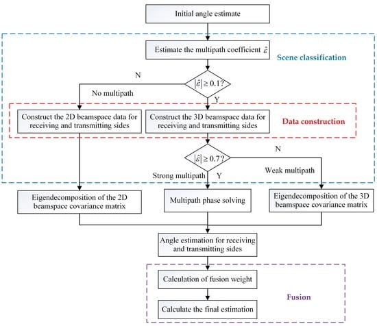
It is worth noting that the closed-form solutions for the weak multipath component and the absence of a multipath component are constrained by the structure of the uniform linear array. Furthermore, the proposed method is only applicable to the scene of a single target in a multipath environment. In a multiple target scenario, multiple targets require separation in the range, Doppler, and angle dimensions through signal processing. The flow chart of the BSC algorithm is summarized in
Figure 2.
2.7. The Simplified Angle-Estimation Method
Furthermore, in the case of , the beamspace data for the receiving and transmitting sides are identical to the two samples of the same signal. Thus, the beamspace data for both the receiving and transmitting sides can be added directly. Then, the solution of the simplified BSC algorithm for target angle can be achieved directly without requiring a fusion process.
3. Results
This section discusses the angle-estimation performances of the BIML, 3D-BMLF, and BSC algorithms, as well as the CRB for refined signal models [
5] through computer simulations.
Consider a narrowband collocated MIMO radar equipped with a uniform linear array. The linear array is mounted vertically in the horizontal plane. The input parameters are set to
,
,
,
, and
. The radar transmits signals with an orthogonal waveform and a bandwidth of 1 MHz. A pulse contains 800 sample points, and the signal envelope follows a Swerling 0 nonfluctuation model. Other simulation parameters are discussed in further detail below. The number of Monte Carlo realizations is set to 500 in each of these simulations. Next, the SNR is defined as
Firstly, the RMSEs of the target angle for each of the three algorithms are shown against the target angle in a flat reflector scene. For
and
, the RMSE of the target angle corresponding to the three algorithms is plotted against the angle and the CRB in
Figure 3. The BSC algorithm outperforms the BIML and 3D-BMLF algorithms, especially in high-angle areas, and the BSC algorithm is closer to the CRB than others. When the angle is small, the RMSE of the three algorithms is greater. In addition, the RMSE fluctuates more significantly for BIML and 3D-BMLF.
Secondly, the influence of the RCA on the estimation accuracy is investigated. Assuming
,
, and
, the RMSEs of the target angle for the three algorithms are plotted against the RCA in
Figure 4, where the RCA=0 indicates that no multipath signal exists in the target echo. The estimation error of the BIML and 3D-BMLF algorithms diminishes as the RCA grows. The BSC algorithm achieves the lowest estimation error when the RCA is large than 0.7 or less than 0.1. When the RCA is small but greater than 0.1, the BSC algorithm performs identically to the 3D-BMLF algorithms in terms of estimation accuracy.
Thirdly, the RMSE of the target angle for the three algorithms is shown against SNR. Assuming
and
, the RMSEs of the target angle for the three algorithms are shown against SNR in
Figure 5. As the SNR increases, the estimation error of the three algorithms reduces. The RMSE of the BSC algorithm is closer to the CRB and is lower than that of the other algorithms. The RMSE of the target angle for the BSC algorithm and the simplified BSC algorithm are plotted against SNR in
Figure 6. As observed, the BSC algorithm performs identically to the simplified BSC algorithm in cases where
.
Fourthly, the RMSE of the target angle for the BSC algorithm under different noise types is shown against the angle. For
and
,
Figure 7 shows the RMSE of the target angle for the BSC algorithm against the angle, where the three noise types are Gaussian white noise with a mean value of zero, Gaussian white noise with a mean value of 0.1, and Gaussian colored noise with a mean value of zero, denoted by GW-0, GW-1, and GC, respectively. As can be observed, the BSC algorithm performs differently under various noise types. The estimation accuracy under colored noise is inferior to the estimation accuracy under white noise.
Fifthly, the influence of the target distance error and the antenna center height error on the accuracy is investigated for the BIML, 3D-BMLF, and BSC algorithms. It is assumed that
and
. For
, the RMSEs of the target angle for the three algorithms are plotted against the target distance error in
Figure 8. For
, the RMSEs of the target angle for the three algorithms are illustrated against antenna center height error in
Figure 9. As can be observed, the influence of target distance and antenna center height errors on the accuracy of these three algorithms is negligible.


