Abstract
Meteorologically observed air temperature (Ta) is limited due to low density and uneven distribution that leads to uncertain accuracy. Therefore, remote sensing data have been widely used to estimate near-surface Ta on various temporal scales due to their spatially continuous characteristics. However, few studies have focused on instantaneous Ta when satellites overpass. This study aims to produce both daily and instantaneous Ta datasets at 1 km resolution for the Jingjinji area, China during 2018–2019, using machine learning methods based on remote sensing data, dense meteorological observation station data, and auxiliary data (such as elevation and normalized difference vegetation index). Newly released Moderate Resolution Imaging Spectroradiometer (MODIS) Collection 6 surface Downward Shortwave Radiation (DSR) was introduced to improve the accuracy of Ta estimation. Five machine learning algorithms were implemented and compared so that the optimal one could be selected. The random forest (RF) algorithm outperformed the others (such as decision tree, feedforward neural network, generalized linear model) and RF obtained the highest accuracy in model validation with a daily root mean square error (RMSE) of 1.29 °C, mean absolute error (MAE) of 0.94 °C, daytime instantaneous RMSE of 1.88 °C, MAE of 1.35 °C, nighttime instantaneous RMSE of 2.47 °C, and MAE of 1.83 °C. The corresponding R2 was 0.99 for daily average, 0.98 for daytime instantaneous, and 0.95 for nighttime instantaneous. Analysis showed that land surface temperature (LST) was the most important factor contributing to model accuracy, followed by solar declination and DSR, which implied that DSR should be prioritized when estimating Ta. Particularly, these results outperformed most models presented in previous studies. These findings suggested that RF could be used to estimate daily instantaneous Ta at unprecedented accuracy and temporal scale with proper training and very dense station data. The estimated dataset could be very useful for local climate and ecology studies, as well as for nature resources exploration.
1. Introduction
Near-surface temperature (Ta) refers to the temperature two meters above the ground, which is an important parameter in many fields such as the studies of the environment [1,2,3], ecology [4], hydrology [5,6], and meteorology [7,8,9,10]. In the context of global warming over the past few decades, accurate estimation of Ta is very important for climate change assessment and global collaborative response and also provides the scientific basis for China’s carbon peak and neutrality goals to address climate change. The Ta is usually obtained from the observations of ground-based weather stations. Although high-resolution and very precise temperature data can be obtained through site observations, obtaining large-scale continuous temperature data through such stations is difficult because these meteorological stations can only provide discrete observational data and the spatial distribution of the stations is not uniform because of variations in geographical conditions [11,12,13]. Low density with an uneven distribution of ground weather stations may lead to inaccuracies and uncertainties in related studies [14,15,16,17].
Before satellite remote sensing technologies were widely used, interpolation was the most common and easy-to-use method for estimating the spatial distribution of Ta, such as Inverse Distance Weighted (IDW), Kriging, Spline method, etc., [18,19,20]. Some methods such as Kriging and Spline can use secondary variables as auxiliary data for interpolation [21,22,23,24,25]. However, the density and uneven spatial distribution of meteorological stations and variation in terrain greatly affect the accuracy of an interpolation algorithm [26,27].
With the development of remote sensing technology in recent decades, estimating large-scale continuous Ta data through satellite remote sensing data has become an important research direction [28,29,30]. The surface temperature (LST) obtained by satellite sensors is spatially continuous, has almost global coverage [31], and has strong correlation with Ta [16,32]. The relationship between LST and Ta is also affected by terrain, elevation, vegetation coverage, and other factors. Many different methods have been proposed to increase the accuracy of satellite-based Ta estimating in recent years [18,33,34]. According to the technical principle, these methods can be divided into four groups:
- Statistical methods such as linear regression models are commonly used to explore the relationship between Ta and other variables [35,36,37,38,39]. Cresswell et al. [40] estimated instantaneous Ta through a multiple regression model; the model used Solar Zenith Angle (SZA) as the only auxiliary variable and achieved an accuracy of mean deviation less than 3 °C for over 70% of the cases. Chen et al. [27] retrieved monthly average temperature (RMSE between 1.29 and 1.45 °C) and eight-day average temperature (RMSE between 0.8 and 1.29 °C) for China in 2010 using a model based on remote sensing data and a geographically weighted regression (GWR) algorithm; the elevation was the only secondary auxiliary variable; the results show that the GWR method performs better than the multiple linear regression method and the regression Kriging method.
- The temperature–vegetation index (TVX) method is based on the characteristics of plant canopy temperature that is close to the Ta; this method can be used to calculate the Ta by the relationship between a vegetation index and LST and has also been widely used [31,41,42]. The TVX method was tested in many areas of the world; the resulting RMSE was between 1–3 °C [41,42,43,44,45]. Due to the principle of the method, the TVX method is more suitable for areas with more vegetation coverage. The TVX method shows significant uncertainties while applied to the area with sparse vegetation [43].
- The energy balance method based on the surface heat flux balance equation, incoming net radiation flux, and anthropogenic heat fluxes equals the sum of outgoing land surface heat flux (sensible and latent heat flux) [46,47,48]. Zaksek et al. [49] carried out an estimation of Ta in Slovenia and Germany using the energy balance method, having the root mean square deviation (RMSD) of the results at 2 °C. The method can well describe the physical mechanism of the near-surface energy balance process [50]. The main drawback of the method is that many environmental data (usually in hourly intervals) were needed to force the model and not all data were easy to obtain, especially in a large scale [48].
- Machine learning (ML) methods (such as neural networks, decision trees, support vector machine) are based on nonlinear machine learning algorithms. ML methods greatly improve the computational efficiency and simplify the exploration process of nonlinear and highly interactive relationships compared with the traditional statistical method, the TVX method, and the energy balance method [51,52,53].
Numerous studies tested the different ML methods in satellite-based Ta estimating in recent years. Noi et al. [41] compared the accuracy of multiple regression model, decision tree model, and random forest model in estimating near-surface air temperature in the mountainous area of northwest Vietnam from 2009 to 2013. The results showed that the decision tree model and the linear regression model performed better than the random forest model when only LST data were used without auxiliary variables. However, when two easily accessible variables (altitude and Julian day) were introduced into the model as auxiliary variables, the decision tree model and the random forest model performed significantly better than the linear regression model, which indicates that the ML method is more suitable for a multi-auxiliary variable model. Yoo et al. [54] used the random forest model to estimate the daily maximum and minimum temperatures in Los Angeles and Seoul and introduced seven auxiliary variables into the model: elevation, solar radiation, normalized difference vegetation index, latitude, longitude, aspect, and the percentage of impervious area. The simulated R2 ranged from 0.72–0.85 and RMSE ranged from 1.1–4.7 °C. Zhou et al. [55] proposed a two-stage RF based machine learning hybrid model to estimate intra-daily Ta of Israel during 2004–2016. First, missing LST pixels were estimated and a gap-free LST dataset was obtained, then the RF model was employed to estimate Ta with different auxiliary variables (six auxiliary variables in stage one and seven auxiliary variables in stage two), which reached R2 0.96, MAE 1.12 °C, and RMSE 1.58 °C. Ruiz-Álvarez et al. [56] compared support vector machines, random forests, multiple linear regression, and Kriging interpolation in estimating the Ta in the DHS region of southeastern Spain and the results showed that RF-based methods are more accurate and their performance improved when spatial components are included. Xu et al. [57] compared the accuracy of ten different machine learning methods in simulating the monthly average Ta of the Qinghai-Tibet Plateau with a 1 km resolution and the result showed that the Cubist model performs better than the other models (RMSE, 1.0 °C; MAE, 0.73 °C). Hrisko et al. [58] simulated the Ta of urban areas in the United States using a regression neural network based on GEOS-16 satellites with a simulation result RMSE of 2.6 °C. Li et al. [59] simulated the monthly average Ta of China from 2001 to 2015 using the RF model; the simulation results had an MAE between 1.15 and 1.44 °C and an RMSE between 1.57 and 1.99 °C.
The following points can be summarized from previous studies: (1) estimating Ta based on remote sensing data is one of the most feasible methods at present, especially in a large scale, (2) multi-auxiliary variables can greatly improve the Ta estimation accuracy, (3) the machine learning methods with multi-auxiliary variables were suitable for remote sensing based estimation of Ta [52,53,56,57]. Instantaneous Ta is very important for meteorological processes and weather forecasts, such as numerical weather simulation, for its better near-real-time feature [56]; however, this study found that most previous studies focused on the estimation of average Ta over a period of time from daily average Ta to monthly average Ta in a large-scale area, while instantaneous Ta was rarely estimated [53,60,61]. Furthermore, instantaneous Ta is more difficult to estimate due to considerable changes in one day [62,63]. Thus, this study aimed to further improve estimation accuracy by introducing the Downward Shortwave Radiation (DSR) product into the model, by using high dense in-situ observation data as training inputs in a large study area over different land cover types, and finally by estimating 1 km resolution instantaneous Ta while satellites overpassed for the purpose of assessing the ability of machine learning methods.
2. Study Area and Data
2.1. Study Area
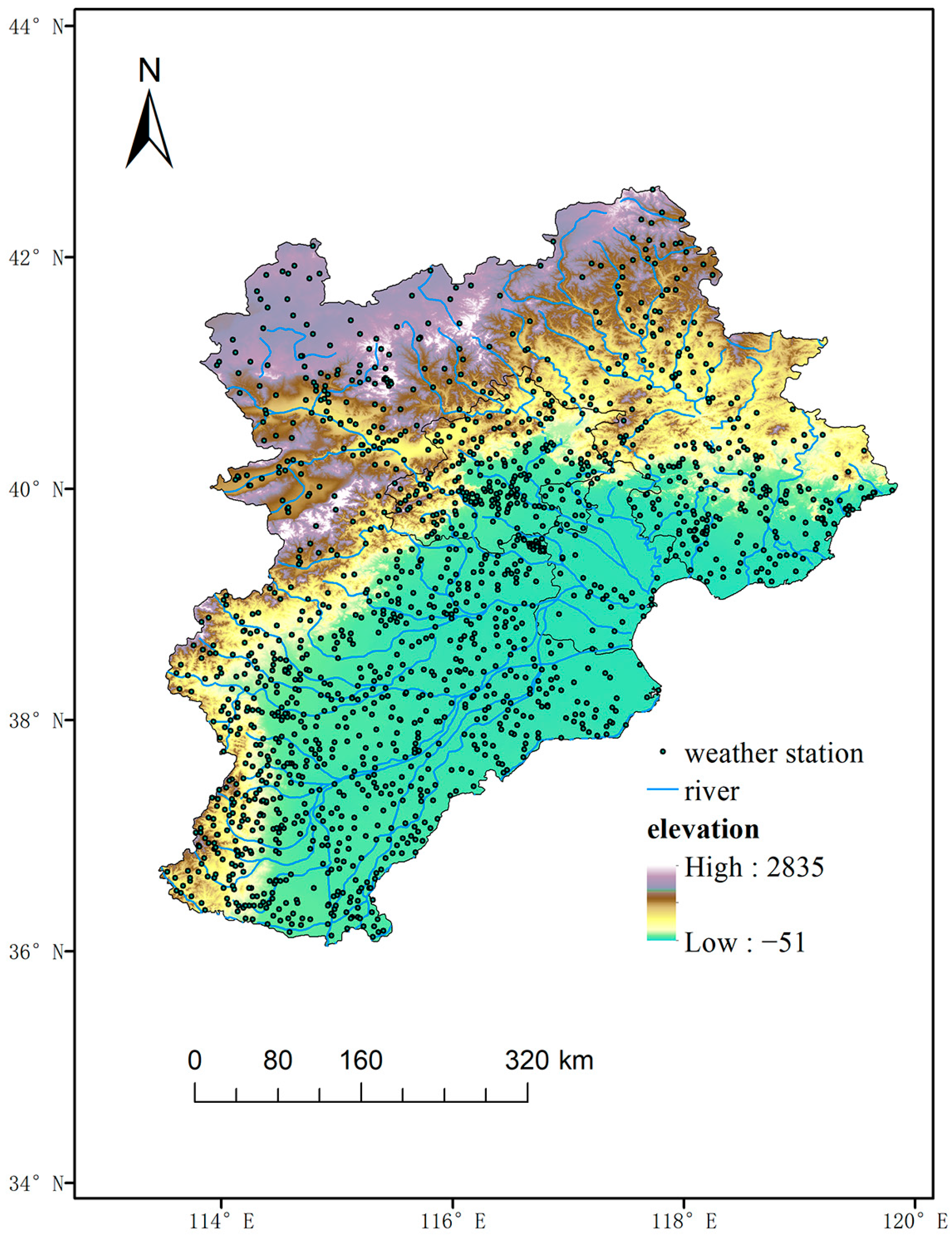
Jingjinji area, located in north China between 36°05′N–42°40′N and 113°27′E–119°50′E, covers three administrative regions including Beijing, Tianjin, and Hebei Province, with a total area of about 218,000 km2 [64] (Figure 1). By 2019, the permanent population was about 113.07 million and the GDP was 8.458 trillion yuan, making it the most important economic core area in northern China. Its terrain is complex and the altitudinal gradient is nearly 3000 m from the northwest mountainous area to the southeast plains area. The land use and vegetation cover are diverse, with a high degree of industrial and agricultural development, including farmland, cities and towns, forests and grasslands, and lakes and wetlands. The rapid urbanization in the Jingjinji area will have an impact on urban heat island and other phenomena. Due to its important status as an economic, cultural, and political center, the Jingjinji area is a hot area of climate change and urbanization research, therefore it is necessary to simulate temperature data. This area has two climatic zones. The northwest belongs to the temperate zone continental climate and the southeast belongs to the temperate zone monsoon climate, which means the Ta estimation is very challenging because of the complexity of the geography. Therefore, factors such as topography, vegetation, and climatic types must be taken into account in the Ta estimation.
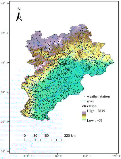
Figure 1.
Location of study area and distribution of meteorological stations.
2.2. Ground-Based Weather Data
The Ta observational data were acquired from the hourly observational data of 1527 weather stations in the Jingjinji region from 2018 to 2019. Figure 1 shows the spatial distribution of the stations. The data quality has been preliminarily controlled according to QX/T 458-2018 meteorological observational data interchange specifications.
2.3. Remotely Sensed Data
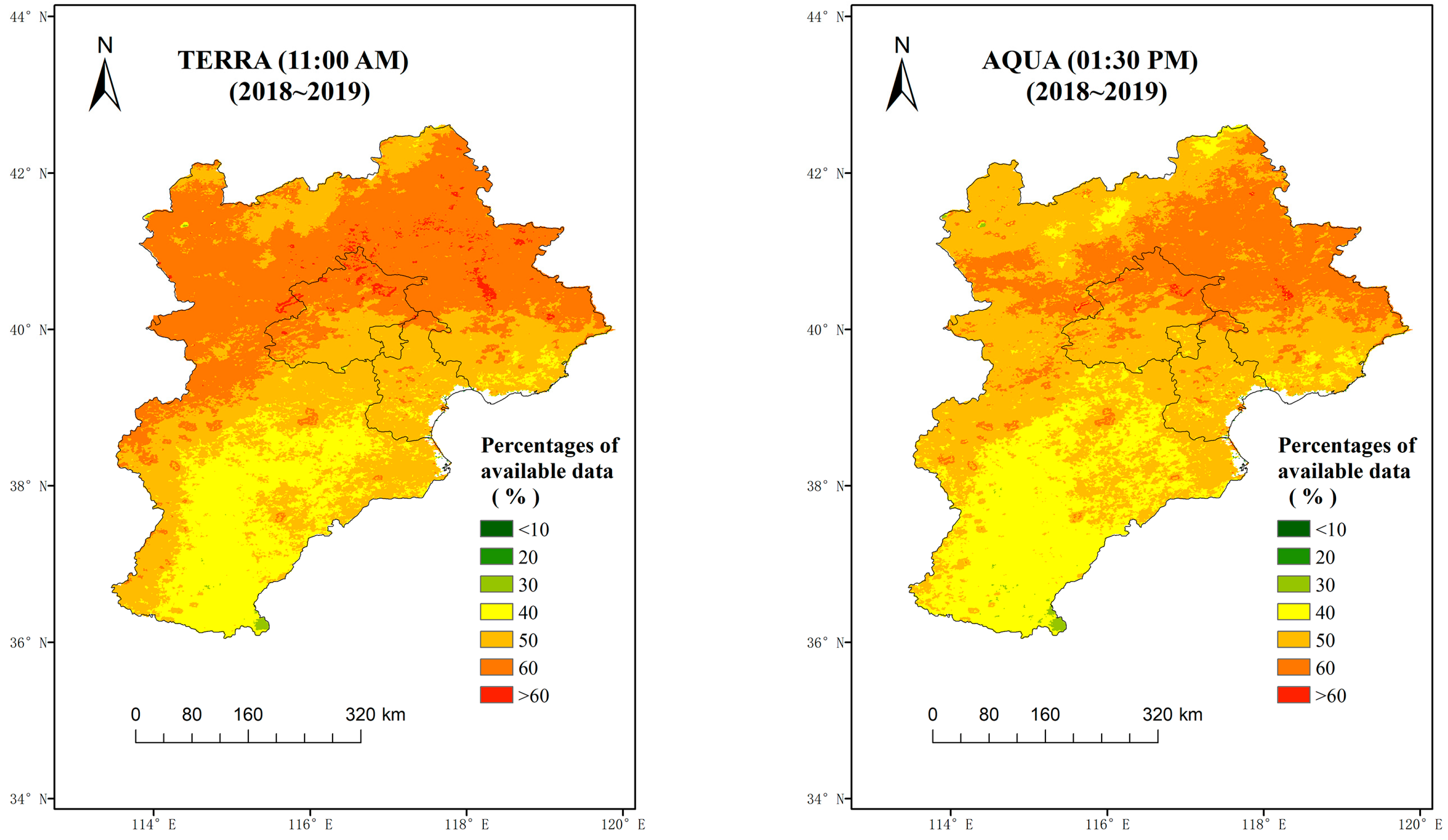
The remote sensing data used in this paper are shown in Table 1. Digital elevation model (DEM) data with a 1 km resolution were produced after secondary processing of the Shuttle Topography Radar Mission’s digital elevation product with a resolution of 90 m. The LST data were derived from MODIS MOD11A1 and MYD11A1 products with a resolution of 1 km released by NASA in 2018–2019. The MODIS remote sensing data come from the infrared radiation sensors carried by Terra and Aqua satellites, which scan the study area twice each day as follows: the transit time of Terra is about 11:00 and 21:00 (Beijing time, also used below), while the transit time of Aqua is about 02:30 and 13:30. Figure 2 show the percentages of available data for each satellite overpass. The mountains in the north and the west have more available data. Data percentage ranged from 50~60%, because high-altitude mountainous areas are less affected by cloud, smog, fog, haze, etc. Overall, the average percentage of valid LST data for the whole study area is about 55%.

Table 1.
Remote sensing data used in this study.

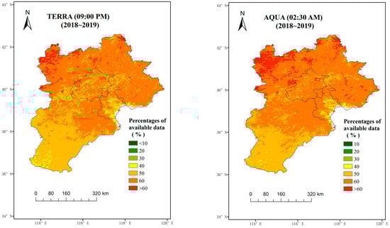
Figure 2.
Average percentages of valid LST data for each satellite pass.
In this paper, three other types of remote sensing data were used as auxiliary input variables in the model, including Downward Shortwave Radiation (DSR), Normalized Difference Vegetation Index (NDVI), and Land Cover (LC) (Table 1). The DSR data were derived from MODIS daily radiation products, numbered MCD18A1 with a spatial resolution of 5 km, according to NASA’s description on its website; the reliability of DSR products has been improved by fixing several errors in the algorithm since 2018. Land Cover data were derived from MODIS annual land cover type data; the product number is MCD12Q1 and has a spatial resolution of 0.5 km. This dataset contains five land cover classification systems. In this paper, the global vegetation classification scheme of the International Geosphere-Biosphere Program was adopted, which divided land cover into 17 types, such as grassland, forest, and water body.
3. Methods
3.1. Variable Selection and Research Framework
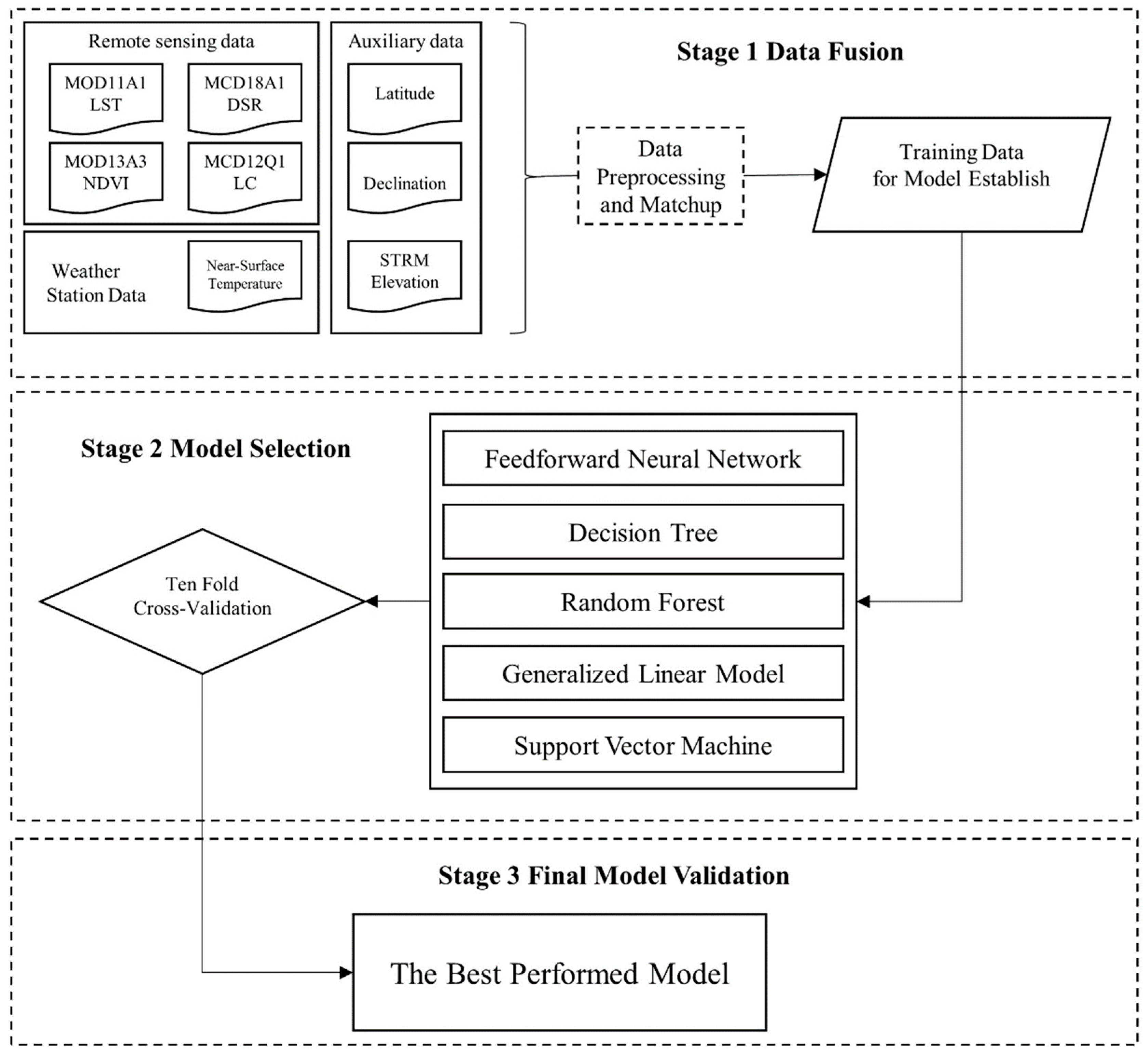
Figure 3 presents the framework of model training and validation used in the present study. As shown in the figure, seven variables (latitude, elevation, declination, normalized difference vegetation index, land cover, downward shortwave radiation, land surface temperature) were selected as model inputs in this study. LST, DSR, NDVI, LC, and digital elevation model data were introduced in Section 2.3. In addition, latitude (LAT) and declination of the sun were selected as auxiliary variables. LAT largely determines the climatic and environmental characteristics of an area, while the declination of the sun is closely related to the day length and seasonal changes of a region. These two factors affect the energy balance process near the ground. Solar declination is rarely considered as a variable in the model of previous studies. This paper ranked the importance of each parameter in the model validation stage in order to verify the importance of different parameters. Table 2 shows the input variables for different scenarios. In this paper, two instantaneous Ta estimation models were established, one for day and one for night. In the estimation of daily mean Ta, the daily mean LST was obtained by summing the LST data of four times a day. If data were missing due to cloud cover or other reasons at a certain time, the daily mean LST of this point was considered as missing.
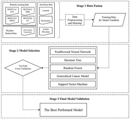
Figure 3.
Flowchart of model training and validation of this study.
Table 2.
Model input variables under different scenarios.
3.2. Models
As both complicated geographic environment and human factors such as impervious land surfaces have influence, Ta changes dramatically along with time and space. Five typical machine learning models were employed to tackle the spatiotemporal variability and factors with complex effects on the relationship with Ta, including a feedforward neural network (FNN) [65], decision tree (DT) [66], random forest (RF) [67], generalized linear model (GLM) [68], and support vector machine (SVM) [69]. We adjusted these models until the lowest level of error was procured using 10-fold cross-validation to obtain best fitting estimation as these models all have different parameter or algorithm combinations. In addition, the final model used for estimating Ta was selected by comparing the performance of the five models (FNN, DT, RF, GLM, and SVM).
3.2.1. Feedforward Neural Network
Feedforward neural network (FNN) is a kind of artificial neural network that has a simple structure and a wide application. It is a kind of static nonlinear mapping, good at complex nonlinear processing [70]. Most feedforward networks are learning networks and their classification ability and pattern recognition ability are generally stronger than those of feedback networks. FNN adopts a unidirectional multilayer structure; each layer contains several neurons and each neuron can receive the signal of the previous neuron and produce the output to the next layer. The zero layer is called the input layer, the last layer is called the output layer, and the other intermediate layers are called the hidden layers; a hidden layer can be one layer or multiple layers [71].
3.2.2. Decision Tree
Decision tree (DT) is a simple but widely used classifier. In machine learning, DT is a prediction model that represents a mapping relationship between object attributes and object values [72]. A decision tree is a tree structure in which each internal node represents a test on an attribute, each branch represents a test output, and each leaf node represents a category. By training data to build a decision tree, the unknown data can be efficiently classified. The decision tree model is readable, descriptive, helpful for manual analysis, and efficient. The decision tree only needs to be constructed once, used repeatedly, and the maximum calculation times of each prediction does not exceed the depth of the decision tree [73].
3.2.3. Random Forest
Random forest (RF), proposed by Breiman in 2001, is a classifier. RF uses multiple trees to train and predict samples. The output categories of RF are determined by the output mode of individual trees [74,75]. RF runs efficiently on large data bases with high accuracy, which can handle thousands of input variables without variable deletion. RF can estimate which variables are important in classification and generate an internal unbiased estimate of generalization error as forest construction progresses. In addition, RF can also effectively estimate missing data and maintain accuracy when the proportion of missing data is large.
3.2.4. Generalized Linear Model
The generalized linear model is based on a linear model; the relationship between the mathematical expected value of a response variable and the predictive variables of a linear combination is established by means of a joint function [76]. It is characterized by the natural measurement of data without forcing changes and data can have nonlinear and unsteady variance structures. It is a development of a linear model in studying non-normal distribution of response value and simple and direct linear transformation of a nonlinear model [77].
3.3. Variable Importance Analysis
Mean decrease accuracy (IncMSE) [78] was used to calculate the importance of different variables in each model. Each model was recalculated to calculate the mean square error (MSE) increment of the new result after a random increase of ±25% deviation for a certain variable, assuming that other conditions remained unchanged. The average value was obtained after 30 repetitions. If the increase in the MSE value was larger, the importance of the parameter in the model was higher; otherwise, the importance was lower.
3.4. Model Training and Validation
In this study, data fusion correction and spatial matching were carried out based on meteorological and remote sensing data from 2018 to 2019. Ultimately, 166,008 daily sample data points and 992,705 instantaneous sample data points were collected. In this study, the widely used 10-fold cross-validation (10-CV) procedure [79] was selected for model validation, where all data samples were divided into ten subsets randomly; nine of them were used as the training data and the remaining as the testing data, and the holdout method is repeated 10 times. We computed an average accuracy score of all the accuracy scores that were calculated in each 10 iterations. The validation of the model was evaluated by mean absolute error (MAE), root mean square error (RMSE), and the coefficient of determination (R2). The statistical measures were defined and used as follows:
where n is the sample size, xi is the simulated value, yi is the measured value, and ȳ is the average value of the measured value.
4. Results
4.1. Comparison of Results of Different Models
We extracted 166,008 samples for the daily model, 456,422 samples for the daytime instantaneous model, and 536,283 samples for the nighttime instantaneous model. Table 3 shows the comparison of simulation results produced by the different models. The results show that the decision tree and RF algorithm performed better than other methods in the model fitting stage; the RMSE of the simulation results of daily mean air temperature, daytime instantaneous Ta, and night instantaneous air temperature ranged from 0.71 °C to 1.42 °C. The RF algorithm is obviously better than other algorithms, while in the model validation stage the RMSEs were 1.29 °C, 1.88 °C, and 2.47 °C, respectively. Therefore, the RF model can be considered as the optimal model in the retrieval of Ta in Jingjinji.
Table 3.
Comparison of results of each model.
According to the results, RF produced the best simulation results for the daily average temperature in the model validation stage with the RMSE, MAE, and R2 of 1.29 °C, 0.94 °C, and 0.99, respectively. Meanwhile, the RMSE, MAE, and R2 of daytime instantaneous Ta simulation were 1.88 °C, 1.35 °C, and 0.98, respectively. The estimation results of instantaneous Ta at night were relatively poor with an RMSE, MAE, and R2 of 2.47 °C, 1.83 °C, and 0.95, respectively (Table 3).
4.2. Analysis of the Importance of Model Variables
Table 4 shows the IncMSE values and the weight ratios of each parameter in different scenarios. The results show that in the simulation of daily mean Ta, the top four variables of IncMSE were LST, LAT, DECLINATION, and DSR. For daytime instantaneous Ta simulation, the top four variables of IncMSE were LST, DECLINATION, DSR, and LAT. For the simulation of nighttime instantaneous Ta, the top four variables of IncMSE were LST, declination, LAT, and LC. In general, the variable LST was much more important than other variables; IncMSE accounted for about 40–60%, followed by DECLINATION, of which the proportion of IncMSE was about 12–28%. In the simulation of daytime instantaneous Ta, the importance of the variable DSR was second only to DECLINATION, and the proportion of IncMSE reached 14.93%, while in the simulation of daily average Ta, the proportion of IncMSE was only 6.63%, which is lower than the variable LAT and DECLINATION.
Table 4.
Ranking of variable importance.
4.3. Evaluation of Random Forest Performance
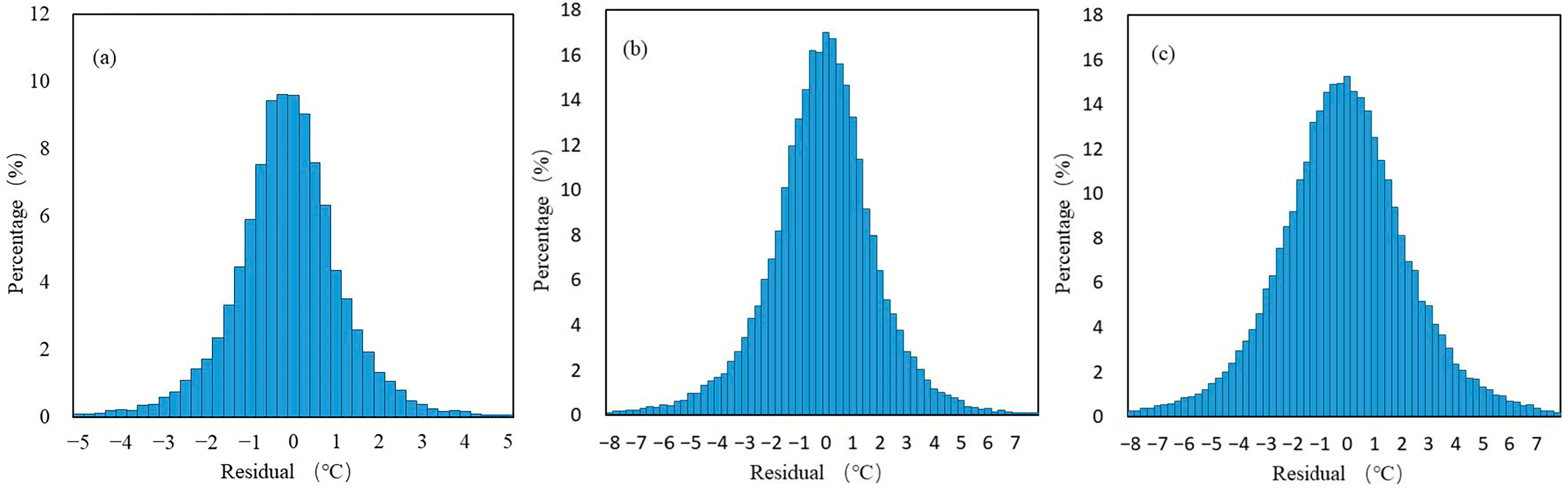
Figure 4 presents the histogram of the distribution validation residuals of daily average Ta, daytime instantaneous Ta, and nighttime instantaneous Ta simulated by the RF model. The figure shows the overall model error has a normal distribution. The error of less than ±1 °C accounts for 64.95%, 50.74%, and 38.09%, respectively, in the simulation of daily average Ta, instantaneous Ta during the day, and instantaneous Ta at night, while the error of less than ±2 °C accounts for 89.18%, 77.86%, and 65.54%, respectively, in the simulation of these three types of Ta.

Figure 4.
Histograms of residuals of the model: (a) daily average near-surface air temperature (Ta), (b) daytime instantaneous Ta, (c) nighttime instantaneous Ta.
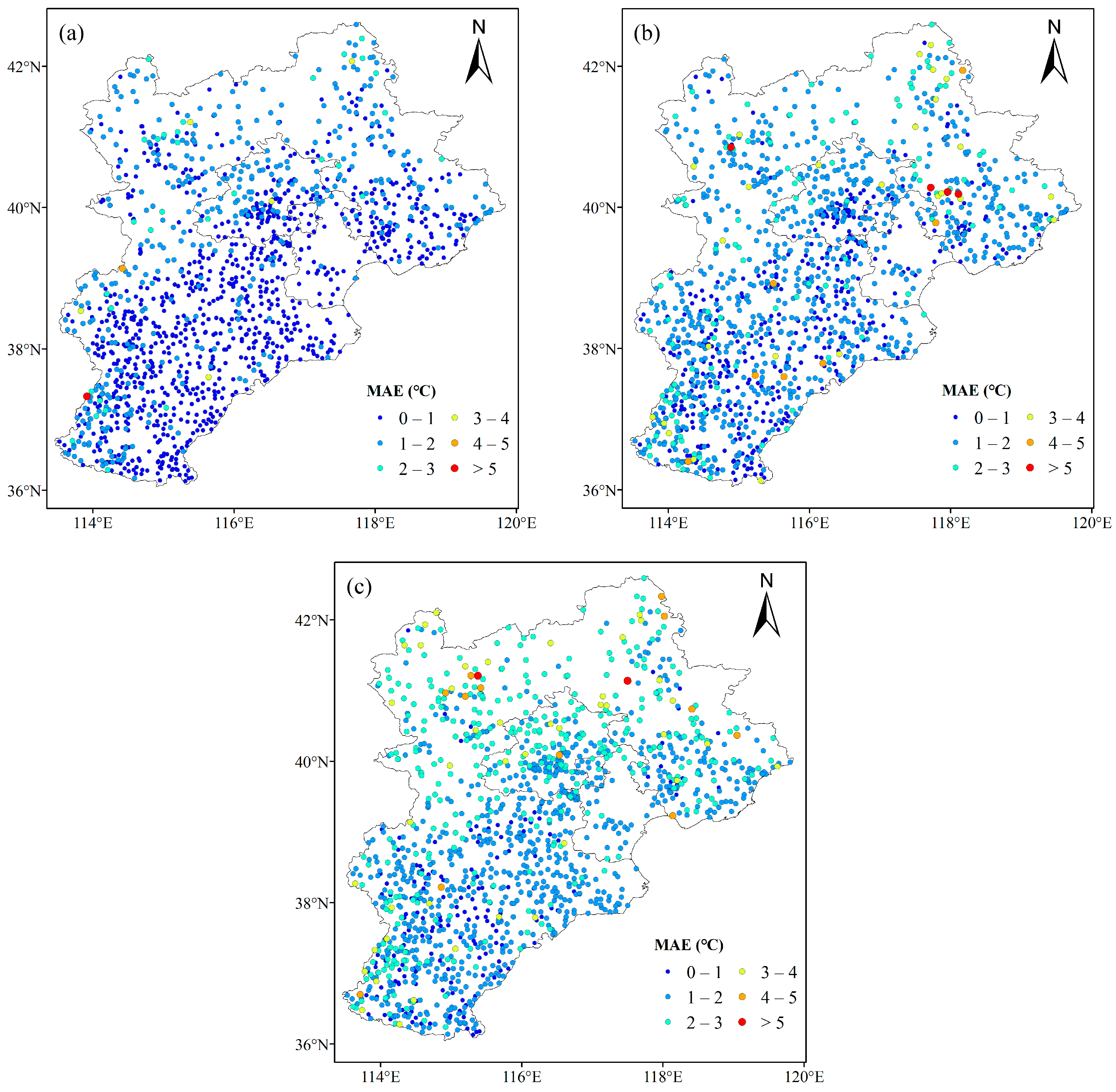
Figure 5 shows a diagram of the distribution of the spatial error in simulation results for daily mean Ta, daytime instantaneous Ta, and nighttime instantaneous Ta under the RF model. As can be seen from Figure 5, when simulating daily average Ta most station errors are between 0 and 2 °C. In the daytime instantaneous Ta simulation, compared with the average daytime Ta simulation, the number of stations with errors of >2 °C increased significantly. In addition, in the simulation of transient Ta at night, the station with error of >2 °C is further increased. According to the spatial distribution characteristics, the sites with errors >2 °C were mainly distributed in the western and northern high-elevation mountainous areas. Table 5 shows the comparison of the simulation results in areas of different types of terrain (plains and mountains) and land cover (urban and rural). It can be seen that the simulation accuracy in the plains was higher than in the mountainous areas under various scenarios; RMSE decreased by 0.62 °C, MAE decreased by 0.49 °C, and R2 increased by 0.01 on average. The simulation accuracy in urban areas was higher than in rural areas; RMSE decreased by 0.24 °C, MAE decreased by 0.16 °C, and R2 increased by 0.01 on average.
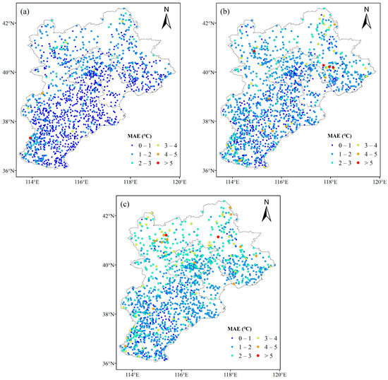
Figure 5.
Mean absolute error (MAE) of estimated near-surface air temperature (Ta) in the Beijing-Tianjing-Hebei region: (a) day average Ta, (b) daytime instantaneous Ta, (c) nighttime instantaneous Ta.
Table 5.
Comparison of the precision of Ta estimation in different types of terrain and land cover.
Table 6 compares the evaluation results of daily average Ta, daytime instantaneous Ta, and nighttime instantaneous Ta at different seasons simulated by the RF model. Figure 6 presents a scatter diagram of simulated and measured Ta values at different seasons. As can be seen from Table 6, in Ta daily average simulation, the error difference in four seasons is generally small. Among them, summer has the best simulation effect, followed by autumn, spring, and winter. The maximum and minimum values of RMSE and MAE in four seasons were 0.32 °C and 0.25 °C, respectively. In the simulation of daytime instantaneous Ta, the simulation worked best in winter, followed by autumn and summer. The simulation results in spring are worse than in other seasons. The simulation of instantaneous Ta worked best at night, followed by autumn. Table 6 shows that in summer the models have low MAE but also low R2 in daily average and nighttime scenes. LST is closer to temperature in summer than in other seasons, which probably caused the small MAE in summer. Due to less cloud cover, there are more clear days in other seasons than in summer and a large number of relatively consistent data enhance the correlation of valid data, which may be the main reason for the high R2 in other seasons.
Table 6.
Comparison of the precision of Ta estimation in different seasons.
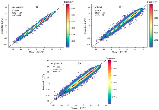
Figure 6.
Scatter plot of simulation of near-surface air temperature (Ta) and observed values in different seasons: (a) daily average Ta, (b) daytime Ta, (c) nighttime Ta.
4.4. Spatial Distribution of Ta
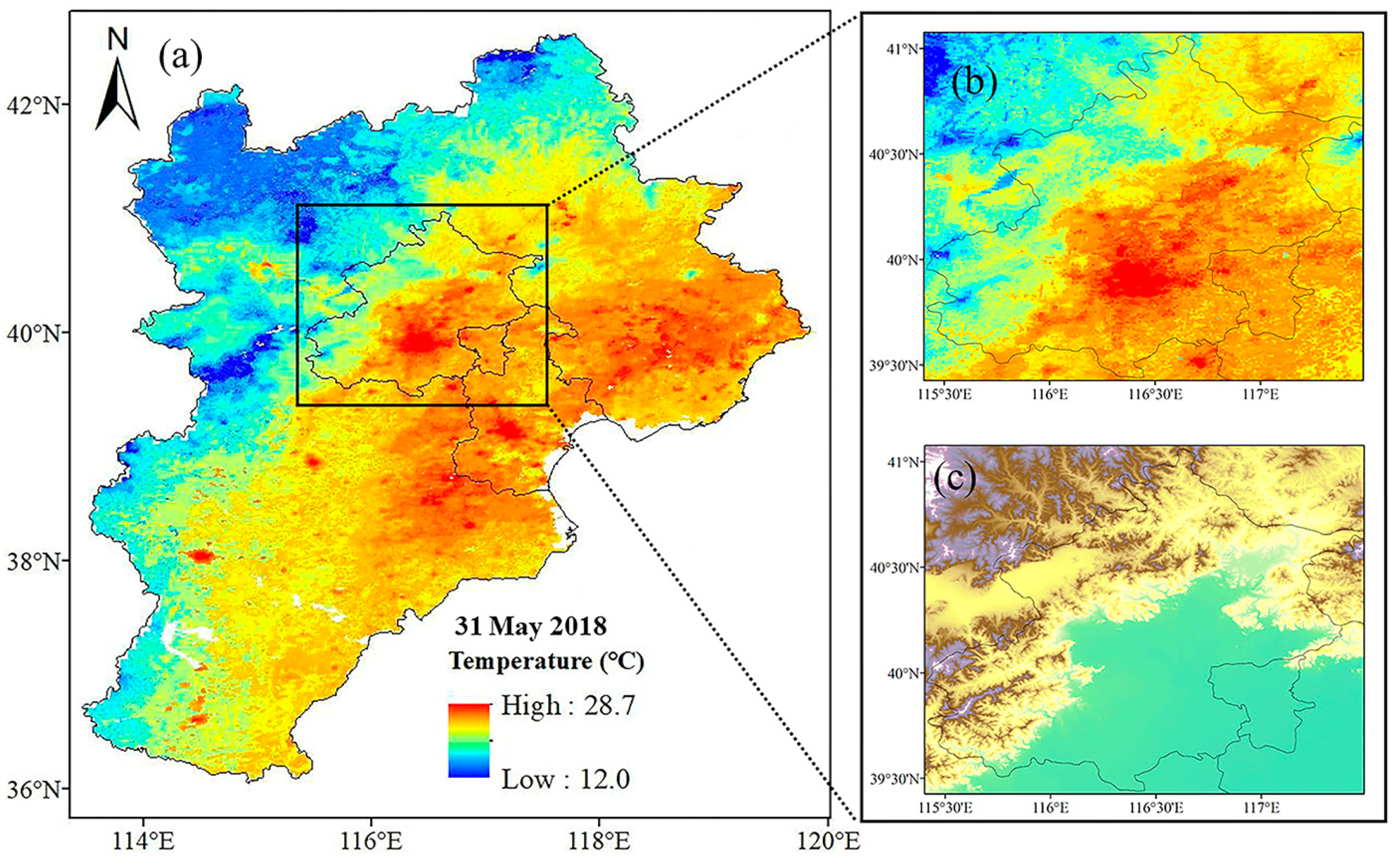
Thirty-first May 2018 was one of the clearest days in the study period. It was selected for showing the model’s ability to recreate spatial Ta distribution maps where ground weather stations do not exist. Figure 7a shows satellite retrieval daily mean Ta of Jingjinji region on the selected day. The result shows that the distribution of high and low Ta is very close to the distribution of elevation, which is consistent with the fact that temperature decreases with height in the troposphere.
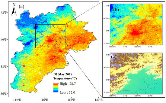
Figure 7.
Comparison between (a) satellite retrieval daily mean temperature of Beijing, Tianjin, Hebei region on 31 May 2018, (b) satellite retrieval daily mean temperature of Beijing area on 31 May 2018, (c) DEM of Beijing area.
The Beijing region was selected for showing the correlation of estimated temperature and the distribution of elevation. Figure 7b contains significant details of the estimated daily mean temperature, which were in line with the distribution of elevation (Figure 7c).
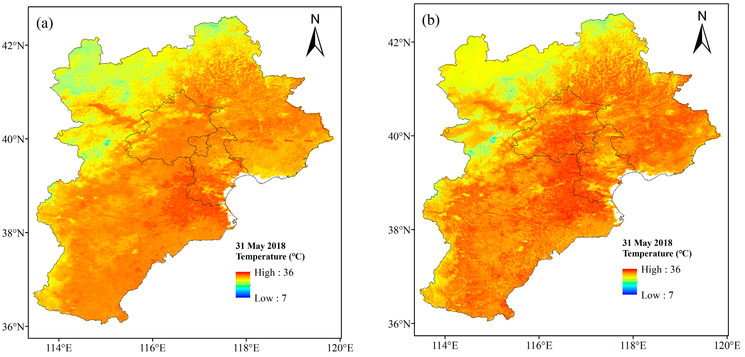
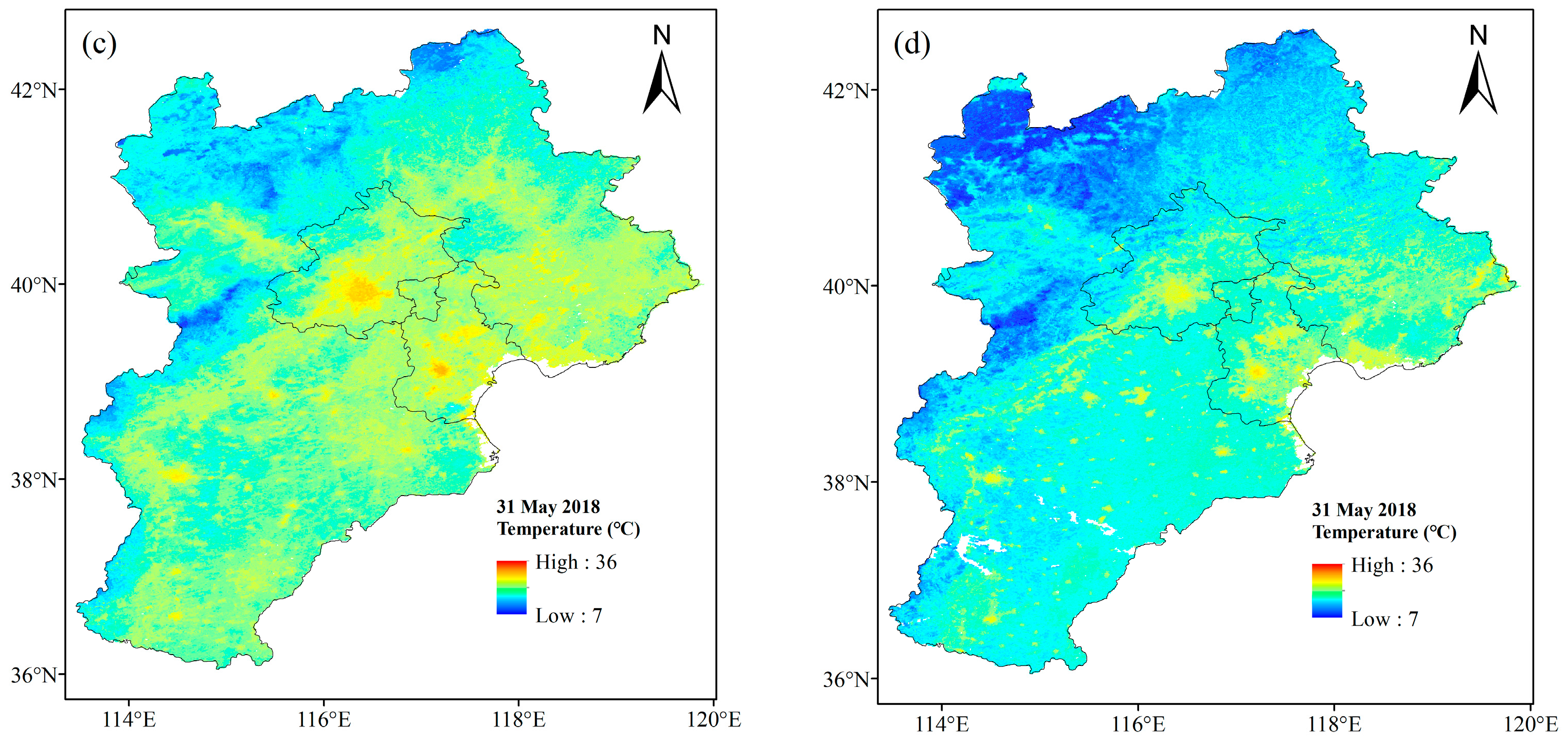
Figure 8 shows the instantaneous Ta estimation products at four times of day on 31 May 2018. This figure shows that the Ta products retrieved by satellite clearly show the process of change in Ta at four times of a day. High Ta areas with clear boundaries caused by the heat island effect are shown after cooling at night.
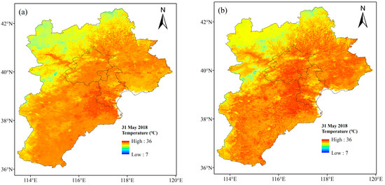

Figure 8.
Daytime and nighttime near-surface air temperature estimation product maps of the Beijing, Tianjin, Hebei region on 31 May 2018: (a) daytime 10:30, (b) daytime 13:30, (c) nighttime 22:30, (d) nighttime 02:30.
5. Discussion
5.1. The Performance of RF Model
This study indicated the RF algorithm is obviously better than other algorithms to estimate daily and instantaneous air temperature from MODIS data over this study area, with the highest accuracy in model validation (Table 3). These results are consistent with other research [52,56,80,81]. In addition, RF produced the best simulation results for daily mean temperature, whereas the results for instantaneous Ta at night were relatively poor. This mainly occurred because the daily average LST was calculated based on four MODIS LST data from two sensors at two local overpass times (daytime and night-time). LST is higher than Ta in the daytime and lower at night, therefore the difference between LST and Ta is greatly reduced after averaging. The poorest simulation results were found at night, mainly because the process of energy balance near the ground at night is quite different from that in the daytime. Phan et al. [61] also found the correlation between LST daytime versus Ta was slightly higher than nighttime versus Ta, which indicated that the relationship between MODIS LST and Ta was complex. In this study, DSR was added as an input variable in the daytime simulation; however, no such variable exists in the nighttime model. Ruiz-Álvarez et al. [56] indicated that the most important variables in RF were satellite land surface temperature, cdayt, and radiation, which could explain the results of this study with lower accuracy observed at night due to the lack of radiation variables compared with the daytime. In addition, this study did not take into account the advection process, which is also a potential factor affecting the instantaneous Ta at night. Specifically, there is no energy at night and the temperature depends on the cooling speed of the air and the ground. The ground and the nearby air are cooled by long wave radiation. On the cloudy night, this long wave radiation is absorbed by the clouds and the clouds also transmit long wave radiation upward and downward, with some of the downward radiation returning to the ground to compensate for heat lost at the ground [82,83]. Therefore, factors such as ground long wave radiation and clouds are affecting the simulation of night temperature and these factors are difficult to quantify using ready-made remote sensing products. Due to the difficulty of data acquisition, these factors were not selected in this study, which led to the phenomenon of low accuracy of night temperature. Therefore, due to the lack of potential influencing factors such as solar radiation and advection processes in the model, the simulation accuracy of instantaneous Ta at night was relatively poor [4,37].
The experimental results of RF showed that the simulation accuracy in the plains area was higher than in the mountainous area (Figure 5). Previous studies also found that the higher the altitude the greater the uncertainty of the model [37], which is mainly caused by the higher elevation, complex terrain, and the process of energy balance near the ground in mountainous areas being more complex [84]. Previous studies have shown that the relationships between daily mean air temperature and LST may change seasonally [85,86,87]. According to the simulation results of different seasons, it was found that the best results among the estimations of daily average Ta and night instantaneous Ta were obtained in summer. However, many previous studies have shown that the estimation accuracy is poorest in summer [37,57,88,89], and this study indicated that this phenomenon can be changed by selecting appropriate variables on the scale of daily average Ta and instantaneous Ta simulation.
5.2. Comparison with Recent Studies
As mentioned in the introduction, many studies have been carried out on the estimation of Ta from remote sensing data. Some studies used machine learning methods that this study follows. Many of them focused on the estimation of monthly average Ta [53,59,80], while other studies focused on estimating the daily average Ta; few studies have focused on the instantaneous Ta. To the best of our knowledge, two such studies [55,56] used a similar method to estimate instantaneous Ta at the satellite pass time. The authors of [55] proposed a two-stage random forest based approach to estimating intra-daily instantaneous Ta across Israel for 2004–2016 and obtained an excellent resulting RMSE of 1.58 °C. The authors of [56] compared four different methods and reached the conclusion that RF performed better than other methods (Support Vector Machines, Multiple Linear Regression, Ordinary Kriging) with the resulting RMSE of 3.01 °C. When compared with studies of daily average validation, the results of this paper are better than most other studies. Table 7 shows the details of comparison with recent studies.
Table 7.
Comparison with recent studies.
Compared with other studies, firstly, we added elevation, which most studies also added [39,55,56,60,90], so this model can be applied to the simulation of temperature under different terrain conditions. Second, we had more stations (1527) than other studies [39,55,56,89,90,91], but fewer than the study of Li et al. [60] (10,141). However, the station density in this study was higher than other studies, therefore the results and process of this current study are still facing uncertainties. It is most likely due to the high density of the site, resulting in high accuracy of the training model. Third, objectively speaking, our model is more suitable for clear-sky days. Cloud cover is a major challenge when modelling air temperature using satellite data. Inevitably, researchers would encounter data missing from satellite-based remote sensing products due to cloud impact or data quality. Since we used MODIS LST products, they had the same defect when it comes to zone under clouds or pixels contaminated by smog, fog, haze, etc. However, none of the currently available satellite-based LST products are spatially continuous due to the presence of clouds, restricting the application of LST and derived Ta based on LST. In the future, we will produce long term Ta products based on gap-free LST products released by other platforms or scholars to make our model applicable to all days not only clear-sky days.
5.3. The Importance of Model Variables
LST can be directly retrieved from remotely sensed radiance data, which is considered as one of the most important and useful data sources for Ta retrieval over a region or large area [92,93,94]. In fact, various studies have used LST data for Ta estimation with high accuracy [37,38,54,80,95]. According to the ranking results of models contributing variable importance, we found that LST was the most important variable affecting simulation results, which was consistent with previous studies [52].
DECLINATION was the second most important variable in the estimation of daytime and nighttime instantaneous Ta and DSR was the third important variable in the estimation of daytime instantaneous Ta only after DECLINATION. Previous studies have rarely used declination as a model input variable. The present study shows that declination is an important parameter for the retrieval of Ta, which is closely related to the change of seasons and the variation of day length; therefore, declination plays an important role in the retrieval of Ta.
Yang et al. [96] indicated that the complexity in land cover, elevation, and solar radiation at daytime could have resulted in low accuracy of Ta estimation, because at night-time there is no solar radiation effect [89,96,97]. During the daytime, the effects of solar radiation will result in a more complex interaction between Ta and LST, which is why the performance of the models with the nighttime LST variable was better than the models without LST nighttime in the study of Phan et al. [61]. In this study, the importance of DSR in the estimation of daytime instantaneous Ta ranks third, which showed that DSR played an important role in the estimation of daytime scenarios and was also one of the reasons why the accuracy of estimation of daytime instantaneous Ta was higher than that of nighttime. As a result, declination and solar radiation are highly recommended to use to improve the accuracy of Ta estimation in the future study.
5.4. Limitations and Future Perspectives
In the estimation of instantaneous Ta, the retrieval accuracy in daytime was obviously better than that at night, which may occur because DSR was added as an input variable of the model in daytime simulation, but there is no such variable in nighttime simulation. In the future, more input variables such as advection processes, wind speed, wind direction, etc., which remote sensors cannot retrieve, should be taken into account and model parameters can be adjusted to further improve the accuracy of nighttime instantaneous air Ta simulation [98,99].
In addition, the results and processes of our current study are still facing uncertainties. Compared with other studies, this study has a high density of meteorological stations, which may have greatly improved the accuracy of the model. In the future, we will attempt to verify the performance of the model in the case of low-density meteorological stations.
6. Conclusions
In this paper, satellite remote sensing data and observational ground-based weather station temperature data in the Jingjinji region during 2018–2019 were used to establish five machine learning models for Ta estimation; the accuracy of the model products was verified and compared. The results showed that RF provided the optimal model with the lowest RMSEs (day average 1.29 °C, daytime instantaneous 1.88 °C, nighttime instantaneous 2.47 °C). In addition, as for the instantaneous Ta estimation, the retrieval accuracy in daytime was obviously better than that at night, the plains areas were obviously better than those in mountainous areas, and the summer simulation results were the best among the Ta estimation of daily average and night instantaneous. This study showed that LST was the most important factor contributing to model accuracy, followed by solar declination and DSR, which implied that declination and DSR should be prioritized when estimating Ta. However, it must be emphasized that there are still several limitations in this study, such as the nighttime instantaneous Ta estimation, which was relatively low due to different surface energy balance processes that occur at night.
In conclusion, based on the support of high-density meteorological station and remote sensing data, a large-scale spatial continuous daily average and instantaneous Ta estimation can be carried out by selecting appropriate variables to establish an RF model. On this basis, the daily average Ta, daytime instantaneous Ta, and nighttime instantaneous Ta datasets with a 1 km resolution in the Jingjinji region from 2018 to 2019 were established in this paper, which can provide spatial continuous Ta data and are of reference value for the boundary layer of related research studies in the Jingjinji region.
Author Contributions
Formal analysis, C.W. and Q.L.; Funding acquisition, Q.L.; Investigation, C.W. and Q.L.; Methodology, Q.L. and C.W.; Project administration, Q.L.; Resources, Q.L.; Software, Z.L.; Supervision, Z.L.; Validation, Q.L. and Z.L.; Writing—original draft, C.W. and X.B.; Writing—review & editing, X.B. All authors have read and agreed to the published version of the manuscript.
Funding
This work was jointly supported by China Meteorological Administration through the Feng-Yun III Satellite Ground Application Project (FY-3(03)-AS-12.09, FY-APP-2021.0408), Beijing Excellent Youth Talent Program, Grant/Award Number: 2015400018760G294, and National Natural Science Foundation of China, Grant/Award Number: 42107498.
Acknowledgments
This research was supported by NASA. The MODIS L1B data were obtained from the NASA/GSFC MODAPS Services website.
Conflicts of Interest
The authors declare no conflict of interest.
References
- Katsouyanni, K.; Pantazopoulou, A.; Touloumi, G.; Tselepidaki, I.; Moustris, K.; Asimakopoulos, D.; Poulopoulou, G.; Trichopoulos, D. Evidence for interaction between air pollution and high temperature in the causation of excess mortality. Arch. Environ. Health Int. J. 1993, 48, 235–242. [Google Scholar] [CrossRef] [PubMed]
- Harvell, C.D.; Mitchell, C.E.; Ward, J.R.; Altizer, S.; Dobson, A.P.; Ostfeld, R.S.; Samuel, M.D. Climate warming and disease risks for terrestrial and marine biota. Science 2002, 296, 2158–2162. [Google Scholar] [CrossRef] [PubMed] [Green Version]
- Koken, P.J.; Piver, W.T.; Ye, F.; Elixhauser, A.; Olsen, L.M.; Portier, C.J. Temperature, air pollution, and hospitalization for cardiovascular diseases among elderly people in Denver. Environ. Health Perspect. 2003, 111, 1312–1317. [Google Scholar] [CrossRef] [PubMed]
- Vancutsem, C.; Ceccato, P.; Dinku, T.; Connor, S.J. Evaluation of MODIS land surface temperature data to estimate air temperature in different ecosystems over Africa. Remote Sens. Environ. 2010, 114, 449–465. [Google Scholar] [CrossRef]
- Lofgren, B.M.; Hunter, T.S.; Wilbarger, J. Effects of using air temperature as a proxy for potential evapotranspiration in climate change scenarios of Great Lakes basin hydrology. J. Great Lakes Res. 2011, 37, 744–752. [Google Scholar] [CrossRef]
- Izady, A.; Davary, K.; Alizadeh, A.; Ziaei, A.; Akhavan, S.; Alipoor, A.; Joodavi, A.; Brusseau, M. Groundwater conceptualization and modeling using distributed SWAT-based recharge for the semi-arid agricultural Neishaboor plain, Iran. Hydrogeol. J. 2015, 23, 47–68. [Google Scholar]
- Smith, W.; Leslie, L.; Diak, G.; Goodman, B.; Velden, C.; Callan, G.; Raymond, W.; Wade, G. The integration of meteorological satellite imagery and numerical dynamical forecast models. Philos. Trans. R. Soc. Lond. Ser. A Math. Phys. Sci. 1988, 324, 317–323. [Google Scholar]
- Willmott, C.J.; Robeson, S.M. Climatologically aided interpolation (CAI) of terrestrial air temperature. Int. J. Climatol. 1995, 15, 221–229. [Google Scholar] [CrossRef]
- Prince, S.; Goetz, S.; Dubayah, R.; Czajkowski, K.; Thawley, M. Inference of surface and air temperature, atmospheric precipitable water and vapor pressure deficit using Advanced Very High-Resolution Radiometer satellite observations: Comparison with field observations. J. Hydrol. 1998, 212, 230–249. [Google Scholar] [CrossRef]
- Robeson, S.M. Relationships between mean and standard deviation of air temperature: Implications for global warming. Clim. Res. 2002, 22, 205–213. [Google Scholar] [CrossRef]
- Xu, Z.; Etzel, R.A.; Su, H.; Huang, C.; Guo, Y.; Tong, S. Impact of ambient temperature on children’s health: A systematic review. Environ. Res. 2012, 117, 120–131. [Google Scholar] [PubMed] [Green Version]
- Li, L.; Zha, Y. Satellite-based regional warming hiatus in China and its implication. Sci. Total Environ. 2019, 648, 1394–1402. [Google Scholar] [CrossRef] [PubMed]
- Li, L.; Zha, Y. Satellite-based spatiotemporal trends of canopy urban heat islands and associated drivers in China’s 32 major cities. Remote Sens. 2019, 11, 102. [Google Scholar] [CrossRef] [Green Version]
- Muller, C.L.; Chapman, L.; Grimmond, C.; Young, D.T.; Cai, X. Sensors and the city: A review of urban meteorological networks. Int. J. Climatol. 2013, 33, 1585–1600. [Google Scholar] [CrossRef]
- Yan, H.; Fan, S.; Guo, C.; Wu, F.; Zhang, N.; Dong, L. Assessing the effects of landscape design parameters on intra-urban air temperature variability: The case of Beijing, China. Build. Environ. 2014, 76, 44–53. [Google Scholar] [CrossRef]
- Pepin, N.; Fowler, H.; Greenwood, G.; Hashmi, M.; Liu, X. Elevation-dependent warming in mountain regions of the world. Nat. Clim. Chang. 2015, 5, 424–430. [Google Scholar]
- Rao, Y.; Liang, S.; Yu, Y. Land surface air temperature data are considerably different among BEST-LAND, CRU-TEM4v, NASA-GISS, and NOAA-NCEI. J. Geophys. Res. Atmos. 2018, 123, 5881–5900. [Google Scholar] [CrossRef]
- Boyer, D.G. Estimation of Daily Temperature Means Using Elevation and Latitude in Mountainous Terrain 1. JAWRA J. Am. Water Resour. Assoc. 1984, 20, 583–588. [Google Scholar] [CrossRef]
- De Beurs, K. Evaluation of Spatial Interpolation Techniques for Climate Variables: Case Study of Jalisco, Mexico. Master’s Thesis, Wageningen Agricultural University, Wageningen, The Netherlands, 1998. [Google Scholar]
- Ishida, T.; Kawashima, S. Use of cokriging to estimate surface air temperature from elevation. Theor. Appl. Climatol. 1993, 47, 147–157. [Google Scholar] [CrossRef]
- Hudson, G.; Wackernagel, H. Mapping temperature using kriging with external drift: Theory and an example from Scotland. Int. J. Climatol. 1994, 14, 77–91. [Google Scholar] [CrossRef]
- Monestiez, P.; Courault, D.; Allard, D.; Ruget, F. Spatial interpolation of air temperature using environmental context: Application to a crop model. Environ. Ecol. Stat. 2001, 8, 297–309. [Google Scholar] [CrossRef]
- Stahl, K.; Moore, R.; Floyer, J.; Asplin, M.; McKendry, I. Comparison of approaches for spatial interpolation of daily air temperature in a large region with complex topography and highly variable station density. Agric. For. Meteorol. 2006, 139, 224–236. [Google Scholar] [CrossRef]
- Wu, T.; Li, Y. Spatial interpolation of temperature in the United States using residual kriging. Appl. Geogr. 2013, 44, 112–120. [Google Scholar] [CrossRef]
- Brunetti, M.; Maugeri, M.; Nanni, T.; Simolo, C.; Spinoni, J. High-resolution temperature climatology for Italy: Interpolation method intercomparison. Int. J. Climatol. 2014, 34, 1278–1296. [Google Scholar] [CrossRef] [Green Version]
- Vicente-Serrano, S.M.; Saz-Sánchez, M.A.; Cuadrat, J.M. Comparative analysis of interpolation methods in the middle Ebro Valley (Spain): Application to annual precipitation and temperature. Clim. Res. 2003, 24, 161–180. [Google Scholar] [CrossRef] [Green Version]
- Chen, F.; Liu, Y.; Liu, Q.; Qin, F. A statistical method based on remote sensing for the estimation of air temperature in China. Int. J. Climatol. 2015, 35, 2131–2143. [Google Scholar] [CrossRef]
- Sun, Y.-J.; Wang, J.-F.; Zhang, R.-H.; Gillies, R.; Xue, Y.; Bo, Y.-C. Air temperature retrieval from remote sensing data based on thermodynamics. Theor. Appl. Climatol. 2005, 80, 37–48. [Google Scholar] [CrossRef]
- Hachem, S.; Duguay, C.; Allard, M. Comparison of MODIS-derived land surface temperatures with ground surface and air temperature measurements in continuous permafrost terrain. Cryosphere 2012, 6, 51–69. [Google Scholar] [CrossRef] [Green Version]
- Kloog, I.; Chudnovsky, A.; Koutrakis, P.; Schwartz, J. Temporal and spatial assessments of minimum air temperature using satellite surface temperature measurements in Massachusetts, USA. Sci. Total Environ. 2012, 432, 85–92. [Google Scholar] [CrossRef] [Green Version]
- Prihodko, L.; Goward, S.N. Estimation of air temperature from remotely sensed surface observations. Remote Sens. Environ. 1997, 60, 335–346. [Google Scholar] [CrossRef]
- Good, E. Daily minimum and maximum surface air temperatures from geostationary satellite data. J. Geophys. Res. Atmos. 2015, 120, 2306–2324. [Google Scholar] [CrossRef]
- An, S.; Zhu, X.; Shen, M.; Wang, Y.; Cao, R.; Chen, X.; Yang, W.; Chen, J.; Tang, Y. Mismatch in elevational shifts between satellite observed vegetation greenness and temperature isolines during 2000–2016 on the Tibetan Plateau. Glob. Chang. Biol. 2018, 24, 5411–5425. [Google Scholar] [CrossRef] [PubMed]
- Wan, Z.; Dozier, J. A generalized split-window algorithm for retrieving land-surface temperature from space. IEEE Trans. Geosci. Remote Sens. 1996, 34, 892–905. [Google Scholar]
- Mostovoy, G.V.; King, R.L.; Reddy, K.R.; Kakani, V.G.; Filippova, M.G. Statistical estimation of daily maximum and minimum air temperatures from MODIS LST data over the state of Mississippi. GIScience Remote Sens. 2006, 43, 78–110. [Google Scholar] [CrossRef] [Green Version]
- Zhang, W.; Huang, Y.; Yu, Y.; Sun, W. Empirical models for estimating daily maximum, minimum and mean air temperatures with MODIS land surface temperatures. Int. J. Remote Sens. 2011, 32, 9415–9440. [Google Scholar] [CrossRef]
- Benali, A.; Carvalho, A.; Nunes, J.; Carvalhais, N.; Santos, A. Estimating air surface temperature in Portugal using MODIS LST data. Remote Sens. Environ. 2012, 124, 108–121. [Google Scholar] [CrossRef]
- Noi, P.T.; Kappas, M.; Degener, J. Estimating daily maximum and minimum land air surface temperature using MODIS land surface temperature data and ground truth data in Northern Vietnam. Remote Sens. 2016, 8, 1002. [Google Scholar] [CrossRef] [Green Version]
- Shi, L.; Liu, P.; Kloog, I.; Lee, M.; Kosheleva, A.; Schwartz, J. Estimating daily air temperature across the Southeastern United States using high-resolution satellite data: A statistical modeling study. Environ. Res. 2016, 146, 51–58. [Google Scholar] [CrossRef] [Green Version]
- Cresswell, M.; Morse, A.; Thomson, M.; Connor, S. Estimating surface air temperatures, from Meteosat land surface temperatures, using an empirical solar zenith angle model. Int. J. Remote Sens. 1999, 20, 1125–1132. [Google Scholar] [CrossRef]
- Nieto, H.; Sandholt, I.; Aguado, I.; Chuvieco, E.; Stisen, S. Air temperature estimation with MSG-SEVIRI data: Calibration and validation of the TVX algorithm for the Iberian Peninsula. Remote Sens. Environ. 2011, 115, 107–116. [Google Scholar] [CrossRef] [Green Version]
- Wloczyk, C.; Borg, E.; Richter, R.; Miegel, K. Estimation of instantaneous air temperature above vegetation and soil surfaces from Landsat 7 ETM+ data in northern Germany. Int. J. Remote Sens. 2011, 32, 9119–9136. [Google Scholar] [CrossRef]
- Czajkowski, K.P.; Goward, S.N.; Stadler, S.J.; Walz, A. Thermal remote sensing of near surface environmental variables: Application over the Oklahoma Mesonet. Prof. Geogr. 2000, 52, 345–357. [Google Scholar] [CrossRef]
- Stisen, S.; Sandholt, I.; Nørgaard, A.; Fensholt, R.; Eklundh, L. Estimation of diurnal air temperature using MSG SEVIRI data in West Africa. Remote Sens. Environ. 2007, 110, 262–274. [Google Scholar] [CrossRef]
- Zhu, W.; Lű, A.; Jia, S. Estimation of daily maximum and minimum air temperature using MODIS land surface temperature products. Remote Sens. Environ. 2013, 130, 62–73. [Google Scholar] [CrossRef]
- Pape, R.; Löffler, J. Modelling spatio-temporal near-surface temperature variation in high mountain landscapes. Ecol. Model. 2004, 178, 483–501. [Google Scholar] [CrossRef]
- Wei, J.; Li, Z.; Li, K.; Dickerson, R.R.; Pinker, R.T.; Wang, J.; Liu, X.; Sun, L.; Xue, W.; Cribb, M. Full-coverage mapping and spatiotemporal variations of ground-level ozone (O3) pollution from 2013 to 2020 across China. Remote Sens. Environ. 2022, 270, 112775. [Google Scholar] [CrossRef]
- Keramitsoglou, I.; Kiranoudis, C.T.; Sismanidis, P.; Zakšek, K. An online system for nowcasting satellite derived temperatures for urban areas. Remote Sens. 2016, 8, 306. [Google Scholar] [CrossRef] [Green Version]
- Zakšek, K.; Schroedter-Homscheidt, M. Parameterization of air temperature in high temporal and spatial resolution from a combination of the SEVIRI and MODIS instruments. ISPRS J. Photogramm. Remote Sens. 2009, 64, 414–421. [Google Scholar] [CrossRef]
- Moran, M.S.; Kustas, W.P.; Vidal, A.; Stannard, D.I.; Blanford, J.H.; Nichols, W.D. Use of ground-based remotely sensed data for surface energy balance evaluation of a semiarid rangeland. Water Resour. Res. 1994, 30, 1339–1349. [Google Scholar] [CrossRef]
- Emamifar, S.; Rahimikhoob, A.; Noroozi, A.A. Daily mean air temperature estimation from MODIS land surface temperature products based on M5 model tree. Int. J. Climatol. 2013, 33, 3174–3181. [Google Scholar] [CrossRef]
- Noi, P.T.; Degener, J.; Kappas, M. Comparison of multiple linear regression, cubist regression, and random forest algorithms to estimate daily air surface temperature from dynamic combinations of MODIS LST data. Remote Sens. 2017, 9, 398. [Google Scholar] [CrossRef] [Green Version]
- Yao, R.; Wang, L.; Huang, X.; Li, L.; Sun, J.; Wu, X.; Jiang, W. Developing a temporally accurate air temperature dataset for Mainland China. Sci. Total Environ. 2020, 706, 136037. [Google Scholar] [CrossRef] [PubMed]
- Yoo, C.; Im, J.; Park, S.; Quackenbush, L.J. Estimation of daily maximum and minimum air temperatures in urban landscapes using MODIS time series satellite data. ISPRS J. Photogramm. Remote Sens. 2018, 137, 149–162. [Google Scholar] [CrossRef]
- Zhou, B.; Erell, E.; Hough, I.; Rosenblatt, J.; Just, A.C.; Novack, V.; Kloog, I. Estimating near-surface air temperature across Israel using a machine learning based hybrid approach. Int. J. Climatol. 2020, 40, 6106–6121. [Google Scholar] [CrossRef] [Green Version]
- Ruiz-Álvarez, M.; Alonso-Sarria, F.; Gomariz-Castillo, F. Interpolation of instantaneous air temperature using geographical and MODIS derived variables with machine learning techniques. ISPRS Int. J. Geo-Inf. 2019, 8, 382. [Google Scholar] [CrossRef] [Green Version]
- Xu, Y.; Knudby, A.; Shen, Y.; Liu, Y. Mapping monthly air temperature in the Tibetan Plateau from MODIS data based on machine learning methods. IEEE J. Sel. Top. Appl. Earth Obs. Remote Sens. 2018, 11, 345–354. [Google Scholar] [CrossRef]
- Hrisko, J.; Ramamurthy, P.; Yu, Y.; Yu, P.; Melecio-Vázquez, D. Urban air temperature model using GOES-16 LST and a diurnal regressive neural network algorithm. Remote Sens. Environ. 2020, 237, 111495. [Google Scholar] [CrossRef]
- Li, L.; Zha, Y. Estimating monthly average temperature by remote sensing in China. Adv. Space Res. 2019, 63, 2345–2357. [Google Scholar] [CrossRef]
- Li, X.; Zhou, Y.; Asrar, G.R.; Zhu, Z. Developing a 1 km resolution daily air temperature dataset for urban and surrounding areas in the conterminous United States. Remote Sens. Environ. 2018, 215, 74–84. [Google Scholar] [CrossRef]
- Phan, T.N.; Kappas, M.; Nguyen, K.T.; Tran, T.P.; Tran, Q.V.; Emam, A.R. Evaluation of MODIS land surface temperature products for daily air surface temperature estimation in northwest Vietnam. Int. J. Remote Sens. 2019, 40, 5544–5562. [Google Scholar] [CrossRef]
- Mira, M.; Ninyerola, M.; Batalla, M.; Pesquer, L.; Pons, X. Improving mean minimum and maximum month-to-month air temperature surfaces using satellite-derived land surface temperature. Remote Sens. 2017, 9, 1313. [Google Scholar] [CrossRef] [Green Version]
- Golkar, F.; Sabziparvar, A.A.; Khanbilvardi, R.; Nazemosadat, M.J.; Zand-Parsa, S.; Rezaei, Y. Estimation of instantaneous air temperature using remote sensing data. Int. J. Remote Sens. 2018, 39, 258–275. [Google Scholar] [CrossRef]
- Chen, P.; Chen, Z.; Yang, X.; Li, B.; Zhang, B. High-resolution land-use mapping in Beijing-Tianjin-Hebei region based on convolutional neural network. In Proceedings of the China High Resolution Earth Observation Conference, Chengdu, China, 1 September 2019; Springer: Singapore, 2019; pp. 213–222. [Google Scholar]
- Bavarian, B. Introduction to neural networks for intelligent control. IEEE Control Syst. Mag. 1988, 8, 3–7. [Google Scholar] [CrossRef]
- Quinlan, J.R. Induction of decision trees. Mach. Learn. 1986, 1, 81–106. [Google Scholar] [CrossRef] [Green Version]
- Breiman, L. Random forest. Mach. Learn. 2001, 45, 5–32. [Google Scholar] [CrossRef] [Green Version]
- Nelder, J.A.; Wedderburn, R.W. Generalized linear models. J. R. Stat. Soc. Ser. A 1972, 135, 370–384. [Google Scholar] [CrossRef]
- Saunders, C. Support Vector Machine. Comput. Sci. 2002, 1, 1–28. [Google Scholar]
- Raeesi, M.; Mesgari, M.; Mahmoudi, P. Traffic time series forecasting by feedforward neural network: A case study based on traffic data of Monroe. Int. Arch. Photogramm. Remote Sens. Spat. Inf. Sci. 2014, 40, 219. [Google Scholar] [CrossRef] [Green Version]
- Tran, D.; Tan, Y.K. Sensorless illumination control of a networked LED-lighting system using feedforward neural network. IEEE Trans. Ind. Electron. 2013, 61, 2113–2121. [Google Scholar] [CrossRef]
- Sun, Y.; Li, X.; Shi, H.; Cui, J.; Wang, W.; Ma, H.; Chen, N. Modeling salinized wasteland using remote sensing with the integration of decision tree and multiple validation approaches in Hetao irrigation district of China. CATENA 2022, 209, 105854. [Google Scholar] [CrossRef]
- Vieira, R.M.d.S.P.; Tomasella, J.; Barbosa, A.A.; Polizel, S.P.; Ometto, J.P.H.B.; Santos, F.C.; da Cruz Ferreira, Y.; de Toledo, P.M. Land degradation mapping in the MATOPIBA region (Brazil) using remote sensing data and decision-tree analysis. Sci. Total Environ. 2021, 782, 146900. [Google Scholar] [CrossRef]
- Pal, M. Random forest classifier for remote sensing classification. Int. J. Remote Sens. 2005, 26, 217–222. [Google Scholar] [CrossRef]
- Belgiu, M.; Drăguţ, L. Random forest in remote sensing: A review of applications and future directions. ISPRS J. Photogramm. Remote Sens. 2016, 114, 24–31. [Google Scholar] [CrossRef]
- Skinner, K.R.; Montgomery, D.C.; Runger, G.C. Process monitoring for multiple count data using generalized linear model-based control charts. Int. J. Prod. Res. 2003, 41, 1167–1180. [Google Scholar] [CrossRef]
- Sahani, N.; Ghosh, T. GIS-based spatial prediction of recreational trail susceptibility in protected area of Sikkim Himalaya using logistic regression, decision tree and random forest model. Ecol. Inform. 2021, 64, 101352. [Google Scholar] [CrossRef]
- Han, H.; Guo, X.; Yu, H. Variable selection using mean decrease accuracy and mean decrease gini based on random forest. In Proceedings of the 2016 7th IEEE International Conference on Software Engineering and Service Science (ICSESS), Beijing, China, 26–28 August 2016; pp. 219–224. [Google Scholar]
- Rodriguez, J.D.; Perez, A.; Lozano, J.A. Sensitivity analysis of k-fold cross validation in prediction error estimation. IEEE Trans. Pattern Anal. Mach. Intell. 2009, 32, 569–575. [Google Scholar] [CrossRef]
- Xu, Y.; Knudby, A.; Ho, H.C. Estimating daily maximum air temperature from MODIS in British Columbia, Canada. Int. J. Remote Sens. 2014, 35, 8108–8121. [Google Scholar] [CrossRef]
- Zhang, H.; Zhang, F.; Ye, M.; Che, T.; Zhang, G. Estimating daily air temperatures over the Tibetan Plateau by dynamically integrating MODIS LST data. J. Geophys. Res. Atmos. 2016, 121, 11425–11441. [Google Scholar] [CrossRef] [Green Version]
- Cao, Q.; Luan, Q.; Liu, Y.; Wang, R. The effects of 2D and 3D building morphology on urban environments: A multi-scale analysis in the Beijing metropolitan region. Build. Environ. 2021, 192, 107635. [Google Scholar] [CrossRef]
- Khesali, E.; Mobasheri, M. A method in near-surface estimation of air temperature (NEAT) in times following the satellite passing time using MODIS images. Adv. Space Res. 2020, 65, 2339–2347. [Google Scholar] [CrossRef]
- Zhao, P.; Xiao, H.; Liu, C.; Zhou, Y.; Xu, X.; Hao, K. Evaluating a simple proxy for climatic cloud-to-ground lightning in Sichuan Province with complex terrain, Southwest China. Int. J. Climatol. 2021. [Google Scholar] [CrossRef]
- Colombi, A.; De Michele, C.; Pepe, M.; Rampini, A.; Michele, C.D. Estimation of daily mean air temperature from MODIS LST in Alpine areas. EARSeL Eproceedings 2007, 6, 38–46. [Google Scholar]
- Sun, D.; Kafatos, M. Note on the NDVI-LST relationship and the use of temperature-related drought indices over North America. Geophys. Res. Lett. 2007, 34, L24406. [Google Scholar] [CrossRef] [Green Version]
- Crosson, W.L.; Al-Hamdan, M.Z.; Hemmings, S.N.; Wade, G.M. A daily merged MODIS Aqua–Terra land surface temperature data set for the conterminous United States. Remote Sens. Environ. 2012, 119, 315–324. [Google Scholar] [CrossRef]
- Kloog, I.; Nordio, F.; Coull, B.A.; Schwartz, J. Predicting spatiotemporal mean air temperature using MODIS satellite surface temperature measurements across the Northeastern USA. Remote Sens. Environ. 2014, 150, 132–139. [Google Scholar] [CrossRef]
- Huang, R.; Zhang, C.; Huang, J.; Zhu, D.; Wang, L.; Liu, J. Mapping of daily mean air temperature in agricultural regions using daytime and nighttime land surface temperatures derived from TERRA and AQUA MODIS data. Remote Sens. 2015, 7, 8728–8756. [Google Scholar] [CrossRef] [Green Version]
- Shen, H.; Jiang, Y.; Li, T.; Cheng, Q.; Zeng, C.; Zhang, L. Deep learning-based air temperature mapping by fusing remote sensing, station, simulation and socioeconomic data. Remote Sens. Environ. 2020, 240, 111692. [Google Scholar] [CrossRef] [Green Version]
- Rao, Y.; Liang, S.; Wang, D.; Yu, Y.; Song, Z.; Zhou, Y.; Shen, M.; Xu, B. Estimating daily average surface air temperature using satellite land surface temperature and top-of-atmosphere radiation products over the Tibetan Plateau. Remote Sens. Environ. 2019, 234, 111462. [Google Scholar] [CrossRef]
- Park, S. Integration of satellite-measured LST data into cokriging for temperature estimation on tropical and temperate islands. Int. J. Climatol. 2011, 31, 1653–1664. [Google Scholar] [CrossRef]
- Li, Z.-L.; Tang, B.-H.; Wu, H.; Ren, H.; Yan, G.; Wan, Z.; Trigo, I.F.; Sobrino, J.A. Satellite-derived land surface temperature: Current status and perspectives. Remote Sens. Environ. 2013, 131, 14–37. [Google Scholar] [CrossRef] [Green Version]
- Chen, Y.; Quan, J.; Zhan, W.; Guo, Z. Enhanced statistical estimation of air temperature incorporating nighttime light data. Remote Sens. 2016, 8, 656. [Google Scholar] [CrossRef] [Green Version]
- Janatian, N.; Sadeghi, M.; Sanaeinejad, S.H.; Bakhshian, E.; Farid, A.; Hasheminia, S.M.; Ghazanfari, S. A statistical framework for estimating air temperature using MODIS land surface temperature data. Int. J. Climatol. 2017, 37, 1181–1194. [Google Scholar] [CrossRef]
- Yang, Y.Z.; Cai, W.H.; Yang, J. Evaluation of MODIS land surface temperature data to estimate near-surface air temperature in Northeast China. Remote Sens. 2017, 9, 410. [Google Scholar] [CrossRef] [Green Version]
- Zeng, L.; Wardlow, B.D.; Tadesse, T.; Shan, J.; Hayes, M.J.; Li, D.; Xiang, D. Estimation of daily air temperature based on MODIS land surface temperature products over the corn belt in the US. Remote Sens. 2015, 7, 951–970. [Google Scholar] [CrossRef] [Green Version]
- Zhao, P.; Xiao, H.; Liu, C.; Zhou, Y. Dependence of Warm Season Cloud-to-Ground Lightning Polarity on Environmental Conditions over Sichuan, Southwest China. Adv. Meteorol. 2021, 2021, 1500470. [Google Scholar] [CrossRef]
- Zhao, P.; Xiao, H.; Liu, J.; Zhou, Y. Precipitation efficiency of cloud and its influencing factors over the Tibetan plateau. Int. J. Climatol. 2022, 42, 416–434. [Google Scholar] [CrossRef]


Publisher’s Note: MDPI stays neutral with regard to jurisdictional claims in published maps and institutional affiliations. |
© 2022 by the authors. Licensee MDPI, Basel, Switzerland. This article is an open access article distributed under the terms and conditions of the Creative Commons Attribution (CC BY) license (https://creativecommons.org/licenses/by/4.0/).