Abstract
This work proposes the use of a robust geometrical segmentation algorithm to detect inherent shapes from dense point clouds. The points are first divided into voxels based on their connectivity and normal consistency. Then, the voxels are classified into different types of shapes through a multi-scale prediction algorithm and multiple shapes including spheres, cylinders, and cones are extracted. Next, a hybrid voting RANSAC algorithm is adopted to separate the point clouds into corresponding segments. The point–shape distance, normal difference, and voxel size are all considered as weight terms when evaluating the proposed shape. Robust voxels are weighted as a whole to ensure efficiency, while single points are considered to achieve the best performance in the disputed region. Finally, graph-cut-based optimization is adopted to deal with the competition among different segments. Experimental results and comparisons indicate that the proposed method can generate reliable segmentation results and provide the best performance compared to the benchmark methods.
1. Introduction
Human-made environments consist of many inherent geometric structures. Understanding them is a principal issue for various applications such as urban reconstruction [1,2,3,4] and indoor scene modeling [5,6]. As the most widely used type of geometric data, point clouds can be derived from various sources, ranging from laser scanners or RGB-D cameras to the stereo-matching of images. Concise and meaningful abstractions of a point cloud into basic structure units will greatly benefit the users’ understanding or further processing [7,8,9,10]. This can often be achieved by a geometric segmentation approach that divides objects into typical shapes [11,12,13]. Currently, segmentation methods can be divided into four categories [14]: edge-based or region growing, feature clustering or classification, model fitting, and deep learning-based segmentation.
Edge- or growing-based approaches [15,16] work by searching for regions that have distinct height or curvature saltations and using them to find a complete edge or determining the stop criterion while growing. These methods are relatively simple and efficient but are prone to errors in the presence of noise or when the transition between adjacent regions is smooth. Techniques using clustering or classification [14] first calculate the feature vector for each point or voxel using elements such as point coordinate, normal, or slope, and then group similar ones. These methods are problematic when deciding the segment number and when noise or tree points close to the segments have not been completely filtered beforehand. End-to-end instance segmentation approaches [17,18] can also be used to segment point clouds into planar instances; their limitations are their need for a large amount of training data and their poor ability in network migration.
Compared with the above approaches, model-fitting methods are suggested to be more efficient and robust in the presence of noise and outliers [19]. RANdom SAmple Consensus (RANSAC) [20] adopts a hypothesis-then-verify fitting strategy which iteratively samples models and verifies them with the remaining data to find the best hypothesis. Numerous variants have been derived from RANSAC; a comprehensive review of these can be found in [21]. For speed, Local-RANSAC [22] via local sampling and Normal Driven (ND) RANSAC [23,24] via normal constraints are used to avoid meaningless hypotheses. Grid voxels are also used in FRANSAC or Voxel RANSAC [25,26]; these can greatly decrease the number of voting terms. For robustness, weighted terms or loss functions can be used to avoid spurious planes, including MSAC, MLESAC [27], and our earlier work [19]. Normal vector consistency [22,24] and spatial connectivity [28] can also be used to validate a hypothesis.
Advances in recent techniques have led to increasingly dense point clouds. This provides the possibility to recognize subtle object details while also creating challenges for current segmentation methods. RANSAC-based approaches have several limitations:
- (1)
- Efficiency with large-scale or dense data. RANSAC methods require a large number of iterations; their point–model consistency and spatial connectivity [29] need to be calculated in each iteration.
- (2)
- Robustness to poor (under-, over-, or no) segmentation or spurious planes [19]. The adjustment of parameters to achieve the best performance is not easy when the point density and object scale are changeable over a large area.
- (3)
- Most current segmentation methods only consider planar segments, while the object shape in a real scene can be much more complex.
In order to tackle the aforementioned issues, a voxel-based RANSAC segmentation algorithm is proposed for the detection of multiple shapes from dense point clouds. The points are first divided into connected point voxels based on the work of [30]. These voxels are then classified and evaluated based on their local features and quality, and multiple shapes, such as spheres, cylinders, and cones are identified, similar to [7]. After the prediction of shape types, a hybrid voting RANSAC approach is used to separate the point clouds into corresponding shapes and fit the parameters. When evaluating the hypothesized shape parameters, voxels with a good quality vote as a whole, which can decrease the voting terms. Others will be decomposed into proper parts and single points, which will vote for themselves. This ensures robustness when voxels are located near the disputable area or when the data quality is poor. Graph-cut-based optimization is also adopted to deal with competition among adjacent shapes and poor segmentation results.
In summary, the contributions of the proposed methods are two-fold: (1) the creation of a hybrid voting strategy to balance the requirements for efficiency and robustness when evaluating the hypothesized shapes; and (2) the creation of a prediction-then-fit strategy to extract multi-shape structures, which can effectively consider the shape scale and shape-type competition. The remainder of this paper is organized as follows. Section 2 describes the related work and Section 3 presents the details of the proposed approach. Section 4 contains an assessment and discussion, and the conclusion is provided in Section 5.
2. Related Work
This section reviews two main issues related to our segmentation approach: (1) voxel clustering, which groups relative points to reduce the number of calculated objects; and (2) existing RANSAC-based point cloud segmentation.
2.1. Voxel Clustering
The concept of the voxel is similar to that of the superpixel in 2D image processing, which provides a natural and compact representation of 3D points. Based on voxels, operations can be performed on regions rather than on single points; thus, this is beneficial for applications that are time-consuming with the original 3D points. Current voxel clustering approaches remain in the development stage, and can be divided into the following categories [30,31], as shown in Table 1:

Table 1.
The categories of voxel clustering methods.
2.1.1. Superpixel-Based 2D Clustering
The superpixel-based approach directly partitions point clouds into a 2D grid or superpixel through horizontal and vertical cutting. Since segmentation for superpixels has already been thoroughly studied in the field of image processing, such as SLIC [32,33] or mean-shift [34], voxels can be easily generated by simply extending them to 3D. Though they have been successfully adopted in video and 3D image segmentation [35], these methods can be problematic when their primitives are uniformly distributed since only 2D information is considered.
2.1.2. Octree-Based 3D Partitioning
Unlike 2D partitioning, the VCCS [26] and VGS [36] algorithms first voxelize the points using an octree and then extract the voxels by evenly partitioning the 3D space. These methods are efficient and can achieve reasonably good results on RGB-D test data. The issue is that their performance is dependent on the voxel resolution and a single voxel may overlap multiple objects; thus, they cannot preserve object boundaries.
2.1.3. Boundary-Enhanced Segmentation
The aim of this category is to better confirm object boundaries in 3D. In the work of [37], points near boundaries are estimated beforehand and their connections are excluded from neighborhood graphs. As a result, the voxels will be separated near the boundaries of objects. Reference [30] formalizes voxel segmentation as a subset selection problem and utilizes the dissimilarity distance term to better extract the boundary locally. The problem is that when the transition between two segments is smooth, the voxel may still overlap two segments. Meanwhile, small objects can be ignored when the voxel resolution has not been properly set.
In our research, voxels with a good quality were taken as integral voting units in the RANSAC-based workflow and boundary-enhanced voxel segmentation by [30] was used. We found that not all the voxels were suitable for voting as a whole based on the following reasons: (1) all points in the scene, including vegetation and noise, are divided into voxels; (2) boundaries may not be well preserved when the transitions between adjacent regions are smooth; and (3) small segments and voxels belonging to curve surfaces are not well considered. As a result, the hybrid voting strategy was used after multiple-scale shape-type prediction on each voxel.
2.2. RANSAC-Based Segmentation
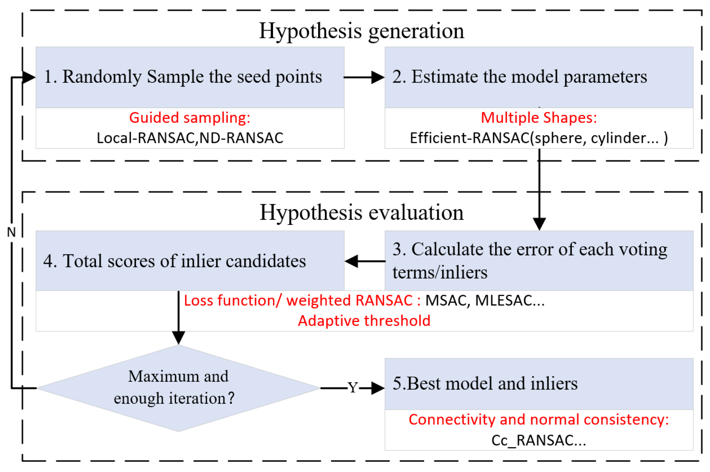
As shown in Figure 1, a standard RANSAC algorithm was used to iteratively and randomly sample points to generate a model hypothesis (hypothesis generation) and then evaluate the model using the remainder of the dataset (hypothesis evaluation). A point was taken as an inlier if its consistency with the hypothesis satisfied a certain condition—i.e., the point–plane distance was smaller than the threshold (step 3). After a certain number of iterations, the shape that possessed the largest number of inliers was extracted (step 5). This method detects planes one by one from the entire dataset, which means that once a plane is accepted, the points belonging to it are removed and the algorithm continues to work on the remainder of the dataset until no satisfactory planes are found. The improvements made in RANSAC-based segmentation are discussed in each step of the workflow [21], which is shown below:
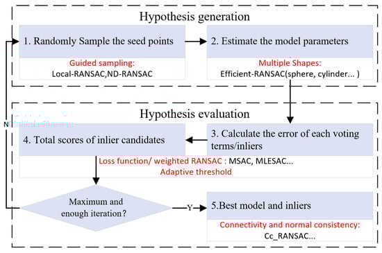
Figure 1.
The workflow of RANSAC and improvements from its variants.
2.2.1. Guided Sampling
Guided sampling works in the hypothesis generation step; its aim is to improve the quality of the hypothesis. Local-RANSAC [22] and ND-RANSAC [23,24] are two classical means used to achieve this goal. Local-RANSAC decreases the sampling space by searching only near the first seed points instead of throughout the whole dataset. ND-RANSAC considers the normal of the seed points and then evaluates the model only when the normals of seeds points are similar to those of the model. These methods can be used to identify meaningless models beforehand, thus avoiding unnecessary hypothesis evaluation.
2.2.2. Multiple Shapes
The RANSAC method can detect any shape in theory as long as the models are defined beforehand and verified through iterations. Though most RANSAC algorithms only consider planar surfaces, a representative implementation of multiple shapes can be found in the work of [7], where curved shapes such as spheres, cylinders, and cones can also be extracted. The major problems experienced are the existence of competition among different shapes.
2.2.3. Loss Function and Weighted RANSAC
The original RANSAC method finds the model with the largest inlier ratio for each iteration, and each inlier makes the same contribution. This might lead to poor segmentation or spurious planes [14,22], especially when the data are noisy or adjacent segments have similar orientations. For weighted RANSAC—i.e., MSAC, MLESAC [27], and our earlier work [19]—a loss function can be identified and points with smaller errors will make a large contribution. Spurious planes with large inlier ratios but smaller total weights will be suppressed, leading to better segmentation results.
2.2.4. Adaptive Threshold
Since most RANSAC methods detect segments one by one from the entire dataset, the inliers need to be moved from the data once a model is accepted. Fixed thresholds are often required to decide the inliers—i.e., the point–model distance and normal difference [24]. The adaptive threshold approach—i.e., [38,39]—is used to estimate the parameters according to the data quality and adjust them while searching for the best proposed models. These methods are more adaptive when the dataset is not consistent over a large area, i.e., stereo matching data whose quality and density are not that reliable.
2.2.5. Connectivity and Normal Consistency
The inlier points detected by RANSAC approaches are mathematically coplanar, though they may not be connected or consistent in space. Density-based connectivity and growing-based normal consistency analysis [22,40,41] can be used in the post-processing step to enhance the segmentation results. In the Cc-RANSAC [29] method, the connectivity is calculated to obtain the most connected component in each iteration, which is robust but time-consuming.
In our work, a classify-then-fit segmentation strategy is proposed; this strategy first identifies the model type and then fits the model parameters. This can help to avoid meaningless competition occurring among different types of shapes; meanwhile, it can decrease the data scale while evaluating the hypothesized shapes. The hybrid voting algorithm can decrease the number of voting terms and increase the robustness under conditions of noise.
3. Methods
First, the overall workflow of the proposed segmentation algorithm is introduced in Section 3.1, followed by the multi-scale shape prediction in Section 3.2. Details of the hybrid voting RANSAC algorithm and the improvements made in connectivity analysis are introduced in Section 3.3. Section 3.4 introduces the graph-cut-based multi-shape optimization method.
3.1. Overall Workflow and Problem Setup
3.1.1. Overall Workflow
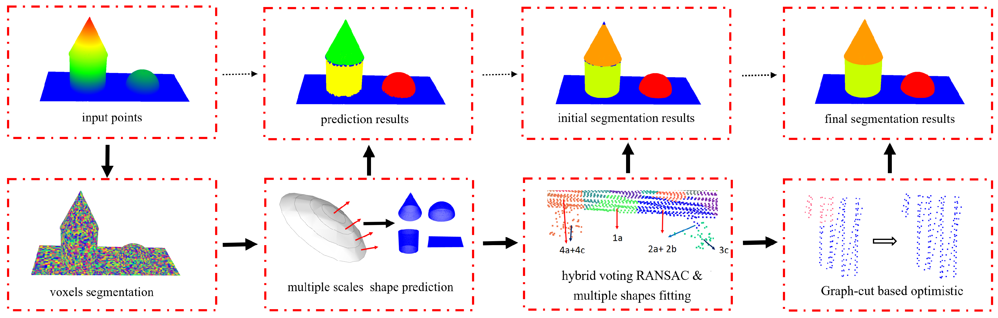
As shown in Figure 2, this method starts with a clustering algorithm that divides the points into voxels based on the work of [30]. These voxels are further evaluated and classified according to their quality and possible shape type, where curved shapes such as spheres, cylinders, and cones are considered. A hybrid voting RANSAC approach is used to separate the points into corresponding segments. Voxel-based connectivity analyses are also introduced to improve the robustness and efficiency in complex scenes. Finally, graph-cut-based optimization is adopted to deal with poor segmentation and spurious shapes.
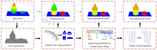
Figure 2.
The overall workflow of the proposed approach.
3.1.2. Problem Setup
Before introducing the details of the proposed methods, we first briefly describe some important terms.
- 3D point P. Basic item, considering its position and normal vectors .
- Super voxel V. A group of points that have similar features and shape types. Each voxel has its centre of gravity and an average normal .
- Observation errors E. The consistency between the point and the proposed shapes, including the distance () and normal difference ().
- Shape type T. Each point or voxel needs to be classified into certain shape types, including planes, spheres, cylinders, and cones.
- Object segment S. A group of points and voxels with the same shape types and segment labels.
The segmentation task carried out in this work needs to separate the point clouds into their corresponding shapes and identify the shape type, which means there are two labels for each P or V: segment index and shape type. Competition among different shape types and parameters need to be applied, and the shapes with the highest scores will be accepted based on the observation errors E regarding and . The V are evaluated in Section 3.2, and the E of high-quality V are evaluated as a whole based on the and . Otherwise, points inside V need to be considered. To avoid the unnecessary competition among different shapes, multi-scale shape predictions are adopted and curve objects are extracted first. Graph-cut-based optimization is used on the final results to produce a global solution.
3.2. Multi-Scale Shape Prediction
Considering that curved surfaces are less numerous in most scenes and are more computationally expensive compared to planar ones, a shape prediction procedure is first adopted for each voxel, and the basic idea is quite simple: propose different shapes and compare them to select the best-performing ones. To ensure efficiency, only the voxel centers are used and the fitting is limited to within the local neighborhood. Below are the details of how we created the hypothesis and performed the evaluation.
3.2.1. Shape Hypothesis
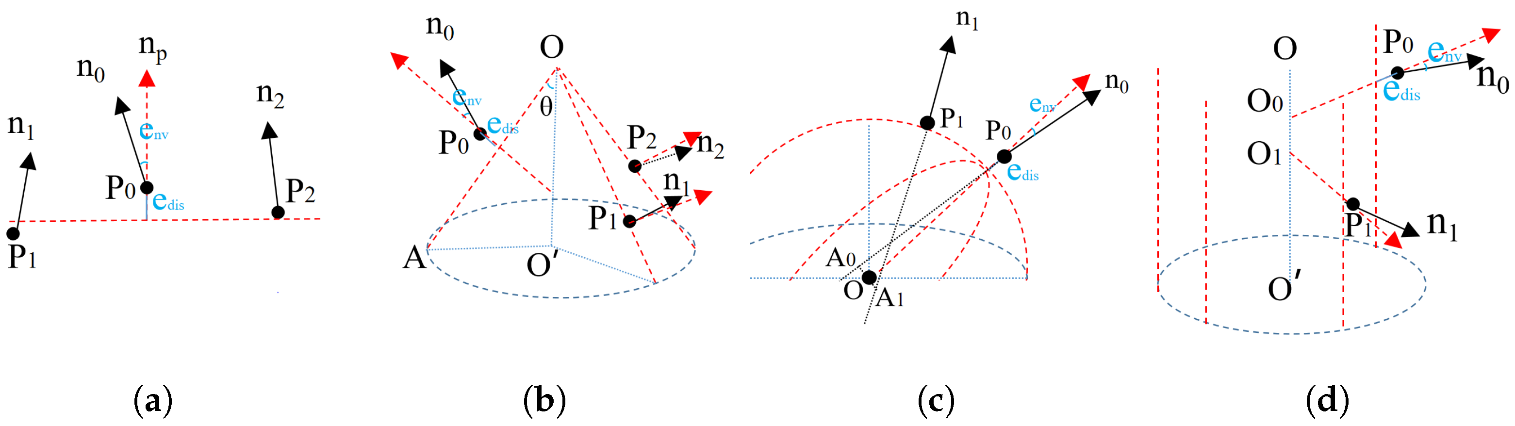
Similar to the work of [7], four types of shapes were included in this work: plane, cone, sphere, and cylinder. Figure 3 shows the definition and samples required to calculate the parameters for different shapes. Since we attempted to predict the shape of the target voxel, was always the first seed and the other seeds were sampled within their neighbors based on the expected shape types and scales. Below are the details of the different shapes; their and were verified before they were proposed as candidates.
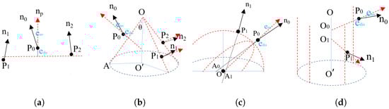
Figure 3.
Definition of different shapes and the required samples. is the gravity center of the target voxel and is that of its random neighbors, and are the normal vectors, and and are the observation errors regarding point-to-shape distance and normal difference: (a) plane, (b) cone, (c) sphere, (d) cylinder.
- Plane. A plane can be estimated using and other two random voxel centers, and .
- Cone. Two more samples, and , with normal vectors are used. Their apex O was intersected by the planes defined from the three point and normal pairs. The axis and the opening angle could from calculated by the average values of normalized , , and . Moreover, if we limit the axis to be vertical in some situations, one sample point will be sufficient.
- Sphere. Another point with anormal vector is required. The sphere center O is the middle point of shortest line segment between the lines defined by the two point and normal pairs and . The sphere radius is the average of and .
- Cylinder. Another sample with a normal vector is sufficient. The axis orientation is defined by . We then project and to the plane vertically to the axis and intersect them for the center. The sphere radius is the average of and .
3.2.2. Shape Evaluation and Prediction
This section evaluates the shapes based on the neighbor voxel centers, where the observation errors E is used to evaluate the performance. Similar to work of [19], the point-to-shape distance and normal difference are considered in the weight function:
where and are two pre-calculated values that reflect the quality of the raw dataset (the distance threshold is considered to be according to [21]). The weight values range from 1 to 0, with an increase in and , which reflects the consistency between the hypothesized shapes and the neighbor voxels, regardless of the shape type.
The prediction procedure iteratively selects the shape type and samples the necessary seeds to calculate the parameters. The most likely hypothesized shape is decided by maximizing the total weights:
where U is the set of selected neighbor voxel centers, which is the same for all scored shapes and parameters. Since objects in real scenes often have a large range of scales, the presence of improper seeds and the neighborhood size will greatly influence the prediction results. As such, multiple scales need to be considered. The workflow of shape prediction is provided below in Algorithm 1:
| Algorithm 1: Shape prediction |
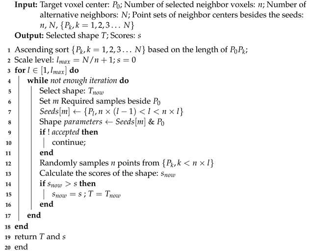 |
The scale level is decided based on the distance between the target voxel center and its neighbors . The random seeds beside are selected from the corresponding scale levels. After a certain number of iterations, a simple winner-take-all principle is used to find the most probable shape type for the target voxel. Voxels with the same shape types are clustered based on their connectivity, and ones that are too small (less than 4 voxels) are converted into planar types.
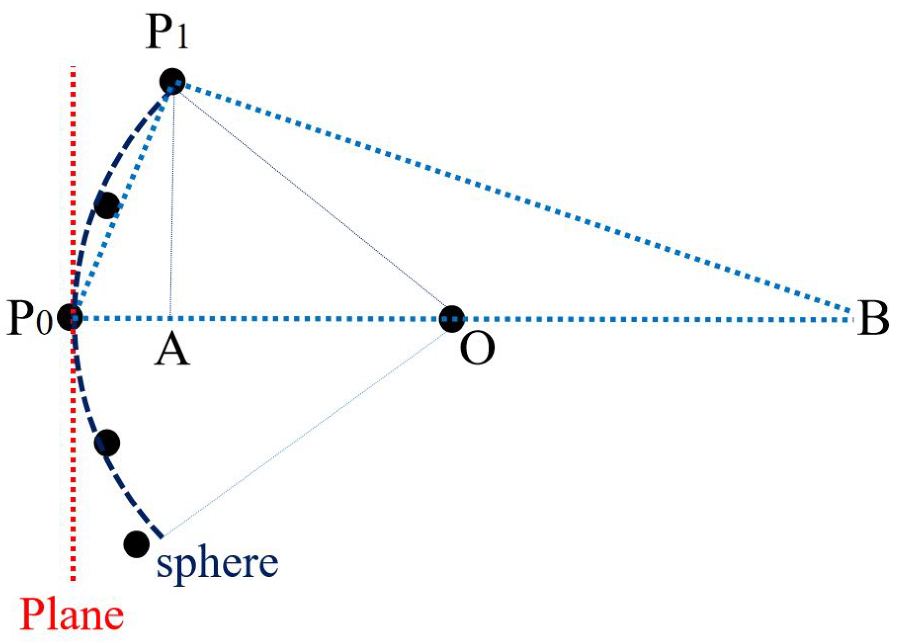
It should be noticed that when the searching scale is much smaller than the local curvature radius, the curved shape will be no longer significant compared to the planar ones. As shown in Figure 4, since the right triangle is similar to :
where is the diameter of the circle equal to and is the distance () between and the farthest neighbor voxel centers. To avoid ambiguous curved shapes, should be larger than the root mean square error ; thus, r should satisfy:
which is changed at the neighborhood scale.

Figure 4.
The competition between planar and curved shapes.
3.3. Hybrid Voting RANSAC-Based Segmentation
The segmentation approaches extract shapes in a subtractive manner, which means that once a shape is detected, the points belonging to it are removed and the algorithm continues on the remainder of the dataset until no satisfactory shapes are found. With the help of the prediction results, target shapes will be detected only from voxels that have the same shape types. The fitting and verification procedures used are similar to those described in Section 3.2; our contribution here is the consideration of voxels in verifying the hypothesis and in the connectivity analysis procedure, instead of using pure point-by-point calculation.
3.3.1. Hybrid Voting
Once the shape prediction approach is completed, we obtain the observation error E between its points and the best shape, diving the points into “good” or “poor” ones. The “good” points will be used to re-calculate the voxel center and normal vectors. If a certain ratio of inliers is taken as “good”, i.e., 80%, the whole voxel will be marked as good and the recalculated voxel centers will be used to represent the whole voxel in the voting step of RANSAC. If less than 20% of the points are marked as “voxel”, the whole voxel will be taken as noise and will only be considered in post-segmentation. Otherwise, it is calculated as a hybrid form: “good” points as a whole and “poor” ones as unit elements. As such, the contribution of a voxel can be expressed as:
where m is the number of points in the voxels and n is the number of “poor” points. n is set as 0 for “good” voxels and and are those for the recalculated voxel center. The weights for hypothetical shapes are defined as the sum of all inside voxels:
For most voxels, their quality is sufficient; thus, the evaluation procedure used can be much faster than point-based approaches. Meanwhile, the possible poor voxel quality at smooth voxel boundaries or noisy areas also needs to be fully considered to obtain robust results. After a certain number of iterations, the models that generate the best evaluation will be extracted.
3.3.2. Voxel-Based Connectivity
The points detected by RANSAC methods are mathematically co-planar but may not necessarily be connected in space. As a result, connectivity analysis is widely adopted in RANSAC-based approaches; this approach is robust but time-consuming, especially for methods such as Cc-RANSAC [29] that check the connectivity in each iteration. In our issue, since the voxels are already defined, it is very convenient for us to check the connectivity at the level of voxels. A graph structure is built, in which the voxel centers are the graph vertexes and the graph edges will connect the adjacent voxels. When analyzing the connectivity, we mark the selected voxels and find the largest connected component within the graph structure. Since the number of voxels is much smaller than the number of point clouds and the graph structure only needs to be constructed once, the efficiency can be ensured.
3.3.3. Post-Segmentation
The main task of the post-processing step is to refine the segmentation results, which includes: retrieving roof points from unsegmented point sets, finding missing planes, and removing false spurious ones. For the voxel-based approach, small roof segments, with a scale closed to the voxel size, mayb e missed during RANSAC segmentation. These segments cannot be easily found during optimization; thus, they must be searched for from the unsegmented point sets. This can be realized through a density-based connectives analysis of the unsegmented point clouds, and an extra fitting procedure is adopted to generate segments with a good quality.
3.4. Graph-Cut-Based Optimization
The optimization of the segmentation results can be taken as an energy minimization problem, and this is often solved by graph-cut-based approaches [9,42,43]. In this work, such procedures are used to solve the competition between different shapes and segments, since they are extracted separately and in a subtractive manner. Meanwhile, the poor (under-, over-, or un-) segmentation caused by improper parameters and noise can also be improved. The energy definition is similar to that of [42], and only voxel centers are considered here:
where data cost measures the discrepancy between the voxel centers and labeled shapes and the smooth cost term considers the inconsistency between neighboring voxels p and q that have different labels, The label cost term measures the number of labels appearing in L.
The difference here in our work is that multiple shapes are considered; thus, the data cost must be updated. On one hand, the point-to-plane distance should be converted into the point-to-shape distance ( in Figure 3), regarding the shape type and parameters. On the other hand, we also consider the normal errors in the data cost, as defined below:
where and are the same as the values given in the RANSAC-based segmentation that represent the quality of the raw dataset. The formulation of smooth cost and label cost is similar to that used in the work of [42] and is not further discussed. The calculation of minimal energy can be solved using the graph-cut technique, which can decide the belonging of voxels and obtain the global best solution.
4. Experimental Evaluations
This section evaluates the proposed methods experimentally. The datasets, parameters, and evaluation metrics are introduced first, followed by the overall results and local details. An analysis and comparison with existing approaches are also provided to verify the performance.
4.1. Dataset, Parameters, and Metrics
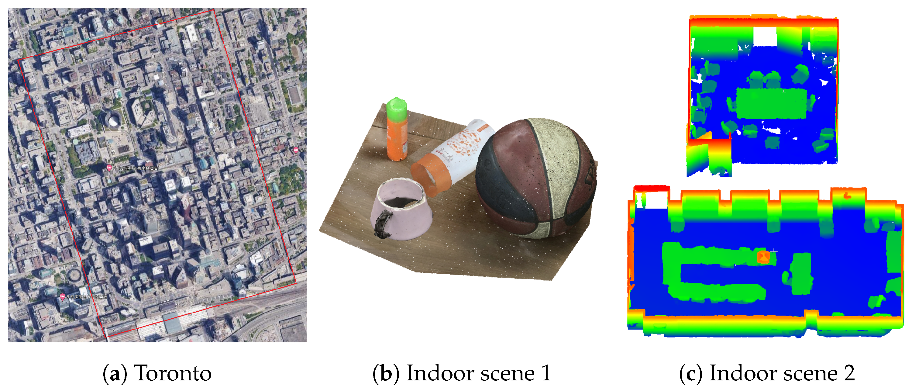
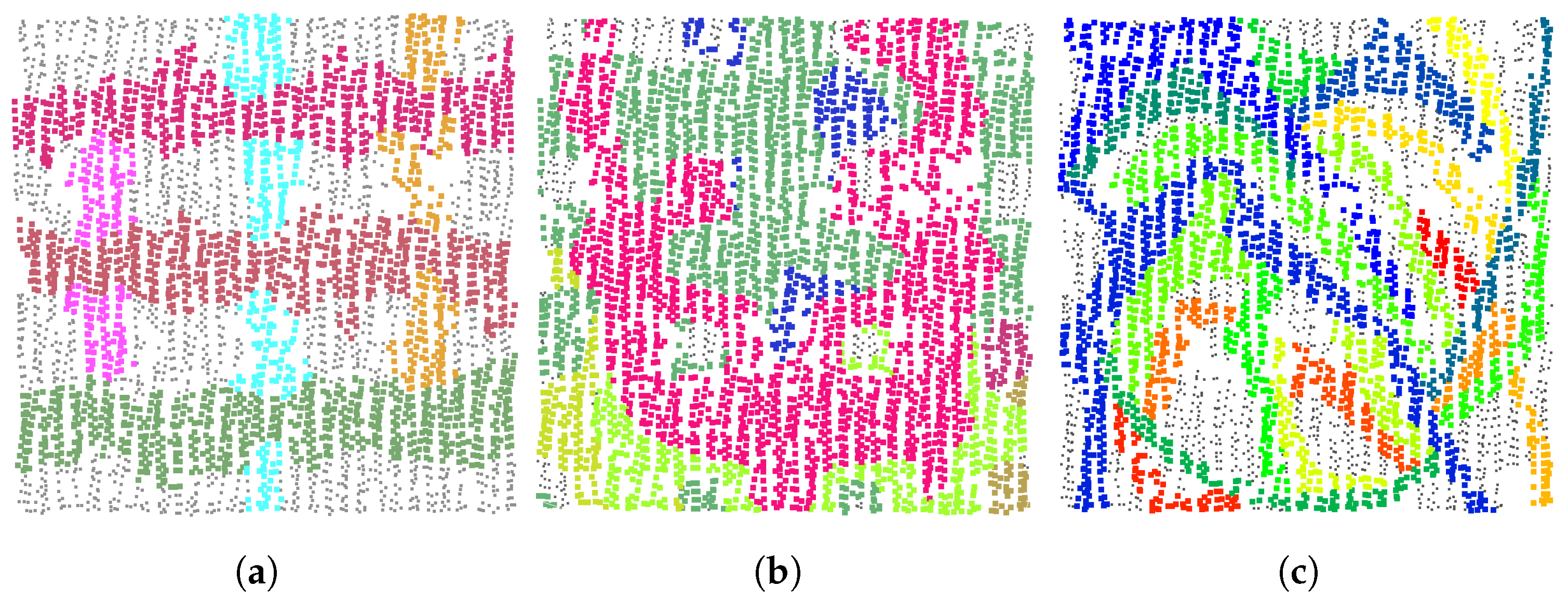
For the experiments, we utilized three datasets, as shown in Figure 5. The first one was selected from the City of Toronto in Canada; it contains the benchmark data from the “ISPRS Test Project on Urban Classification and 3D Building Reconstruction” [44], and contains representative scene characteristics of the modern megacity with a wide variety of rooftop structures. Only the building points are considered here for evaluating our segmentation performance for 3D building reconstruction. The second one is an indoor scene containing multiple objects with different shapes, generated by the dense matching of more than 20 close-range images using the Colmap software. The third one is two rooms selected from the Stanford 3D Dataset [45]; it consists of indoor scenes containing objects such as desktops and chairs. These datasets are used to test the performance in various different scenes. The basic information of the three datasets is introduced in Table 2.
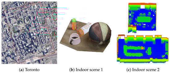
Figure 5.
The introduction to the datasets: (a) The ISPRS benchmark data from the city of Toronto, ON, Canada; and (b,c) indoor scenes created by the matching of close-range images.
Table 2.
The properties of the datasets.
The parameters used in the proposed approaches are described in Table 3. The distance and normal vector thresholds are used for the shape prediction, RANSAC segmentation, and optimization procedure; they are the same and are adjusted according to the data quality.
Table 3.
The parameters used in the experiments.
The evaluation metrics include three parts: the object-level segmentation precision [46], the quality of topology between adjacent shapes [19], and the precision in detecting curved shapes. All of the considered elements use the completeness (Comp), correctness (Corr), and quality (Qua) as metrics:
where (True Positive) is the number of objects that exist in both the reference and results, (False Positive) is the number of objects not found in the reference, and (False Positive) is the number of objects not found in the results.
4.2. Overall Segmentation Results
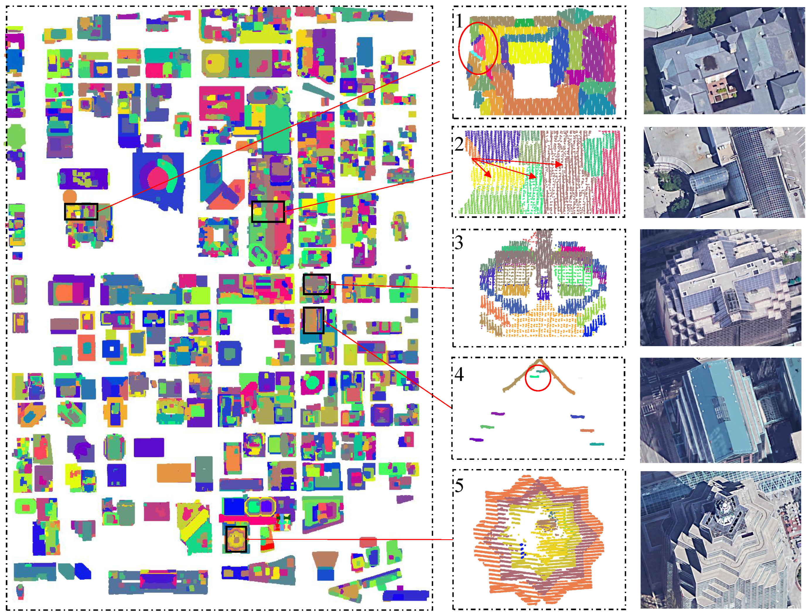
The overall segmentation results obtained for the Toronto dataset are provided in Figure 6. The test area contains various shapes with multiple scales and different styles; these exist not only on the rooftops but also on the vertical walls. The error-prone regions are designated and enlarged to demonstrate the details, and it can be seen that curved shapes with various scales are successfully extracted. Big curved surfaces are completely extracted and the small details are also successfully extracted—i.e., the small segments in enlarged region 1 and cylinders are enlarged in 2. Additionally, the proposed methods can deal with buildings with complex shapes and roof topologies—i.e., there are slender roofs in regions 3 and 5 and the overlapping segments in region 4. More details and a comparison with other researches will be provided later.
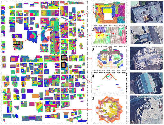
Figure 6.
Overall segmentation results. From left to right: segmentation results, enlarged details, and corresponding Google images.
4.3. Local Details and Precision
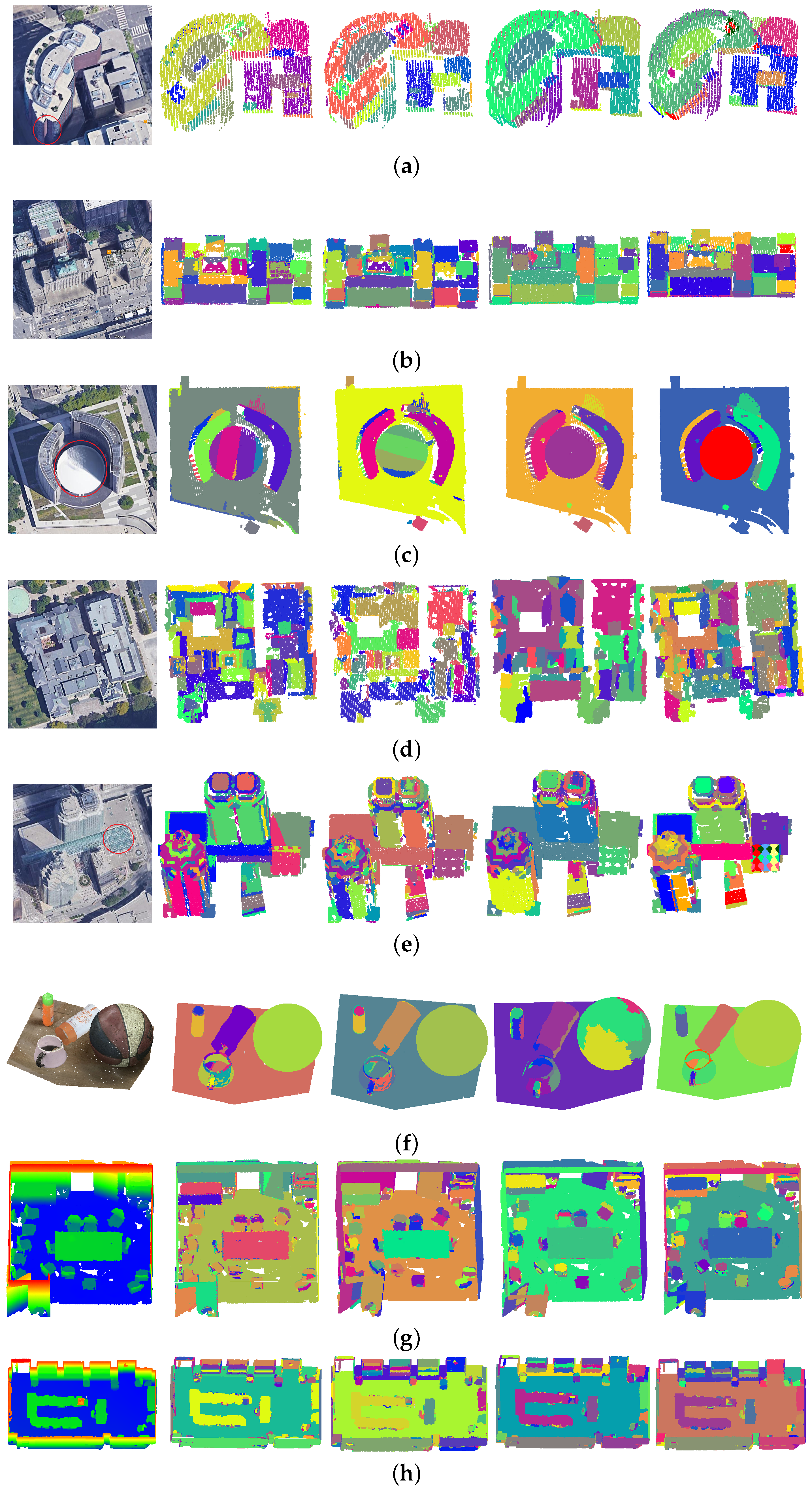
Figure 7 demonstrates our segmentation results obtained in the local scene and compares them to those of existing research. Since the segmentation approaches shown in the Point Cloud Library (PCL) [15] only work on planar surfaces, we adopted efficient RANSAC first [7] for the curved parts and then evaluated the combined results. The Toronto data and the indoor point cloud were compared. Quantitative results are provided in Table 4. The overall performance demonstrates that our methods outperform the other two compared results, and the overall completeness and correctness reached 89% and 88%, respectively.
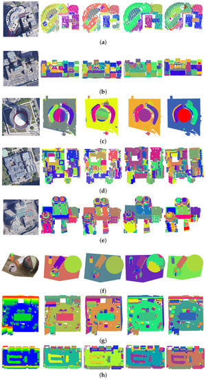
Figure 7.
Segmentation details and comparison with the results of other research, from left to right: Google/input images; results obtained for efficient RANSAC, RG+efficient RANSAC, GlobalL0; and our final results. (a–e) are selected from the Toronto dataset, (f) and (g,h) are the segmentation results of Indoor scene 1 and 2, accordingly.
Table 4.
Comparison of the segmentation results.
The local details also demonstrate the performance of the proposed approach. Buildings Figure 7a,c contain several vertical cylindrical walls and sphere rooftops, which can be successfully predicted and extracted. Especially for the sliders and small features, the efficient RANSAC is very likely to fail by being broken into several parts and making spurious ones. Buildings Figure 7b,d have many small planar segments and complex roof topologies. Voxel-based approaches will face difficulties under such situations, especially when the voxel size is close to that of the segments. Our methods still obtained appropriate results, benefiting from the hybrid voting strategy and the graph-based optimization. Moreover, in the post-segmentation approach, we also try to find the missing segments based on the connectivity analysis of the unsegmented point clouds. Figure 7e consists of several high-rise roofs with very complex shapes and slender structures, as well as noise points on the rooftop. For the six intersecting cylinders in the marked area, a plane overlapping the top of these cylinders is falsely extracted. Our methods show advantages in such situations, and they are correctly classified as cylinders and successfully extracted. For the close-range data shown in Figure 7f, the main curve structures are successfully extracted, including the cone of the cup. The performance of Global-L0 method in Figure 7f is poor, due to the fact that it dose not make curve hypothesis.
For Figure 7g,h, it causes a great deal of trouble compared to current methods, and the quality scores are all less than 80%. This is because of the existence of irregular objects such as chairs, which can be hard to describe through simple shapes. For efficient RANSAC, it has a poor performance due to the lack of spatial connectivity analysis. As a result, chair planes are merged, causing a low level of completeness. For our methods, since the voxels are used, small broken pieces are more likely to be avoided, leading to a high level of correctness. Moreover, our methods can generate a far higher ridge quality, 20% higher than that of the test, benefiting from the graph-cut-based optimization and the boundary-preserved voxel segmentation. This will be of great benefit to the follow-up modeling approach. In conclusion, our methods can generate more robust results under varous scenes; thus, they can obtain the highest overall quality possible, which is 10% higher than that of Global-L0 in the test.
4.4. Parameter Sensitivity
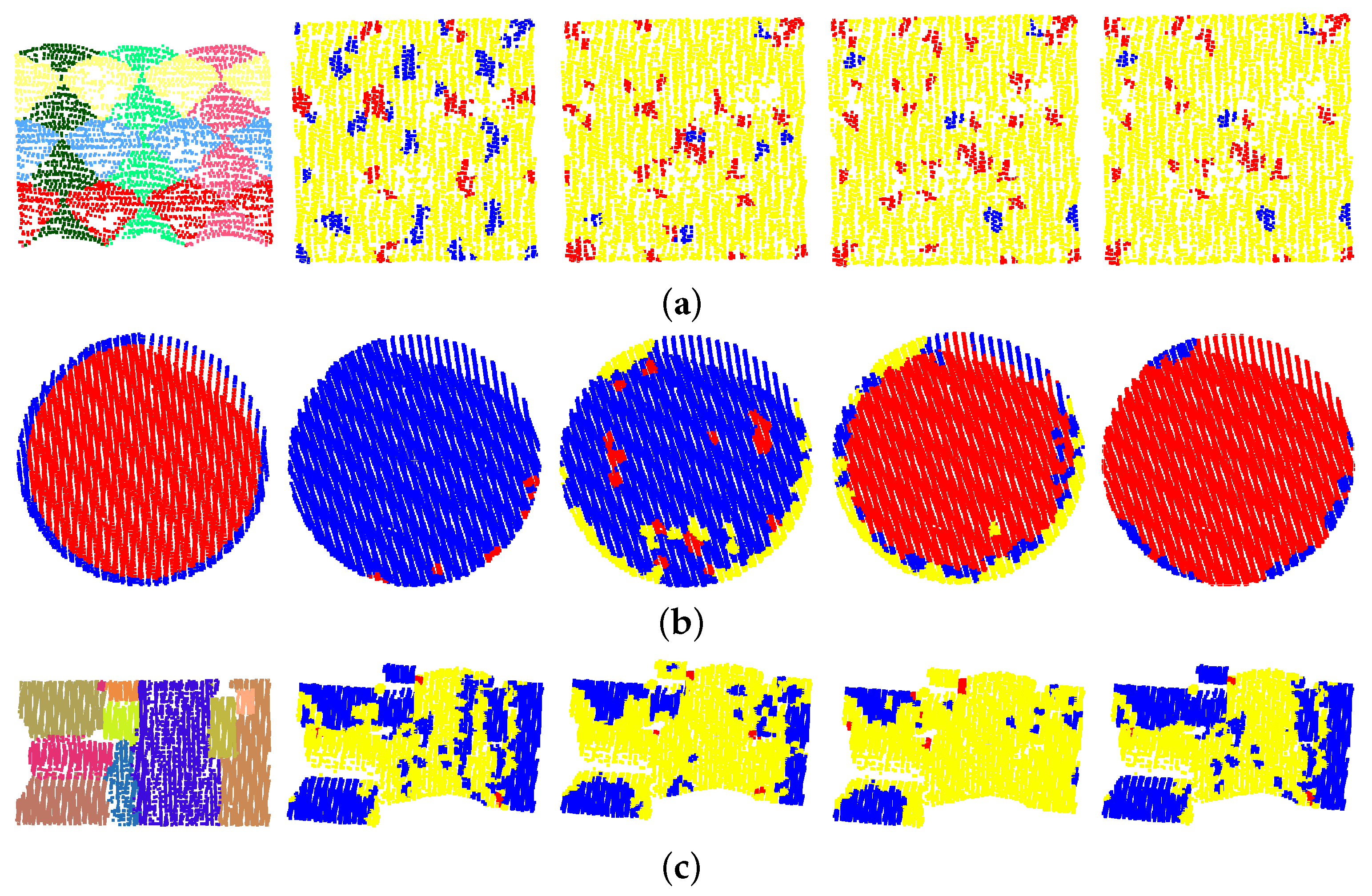
In a local analysis approach, shape prediction may be influenced by the scale of the selected neighborhood. Generally, using a neighbor size that is too small will cause ambiguity between curved shapes and planar ones, leading to noisy prediction results. Meanwhile, using large neighbor size will lead to errors at shape boundaries and cause small objects to be missed. The adaptive neighborhood used in our approach will decrease such influence and produce better prediction results. As shown in Figure 8, three error-prone roofs are selected. Roof a consists of six small cylinders, three horizontal and three vertical and intersected with each other, which can be difficult for both prediction and detection. The locations where two vertical cylinders intersect can be falsely identified as planar surfaces, and the holes between four cylinders may be detected as a sphere when the neighborhood size is set to 10. With the increase in the neighbor size, planar prediction results will become lower and more spheres will appear. Our methods can produce fewer errors, since adaptive scales are more likely to find the most appropriate fitting result. It should be noticed that all the results here are sufficient for the segmentation and fitting, since most points are recognized as cylinders and the clustering of voxels will remove discrete errors. Roof b is a half-sphere with a horizontal eave, and the prediction results at small scales failed because of the limitation provided in Figure 4, where the use of planar surfaces and spheres is controversial. Since the scores of spheres at large scales fit the points better, they can still be successfully identified as spheres. At roof c, three cylinders with different radii are clustered together. What makes this situation worse is that the data quality of the nearby planar surfaces is poor. As a result, some planer voxels are also detected as cylinders. Our methods are also robust under such situations, since the scores achieved under smaller sizes are better in such situations.
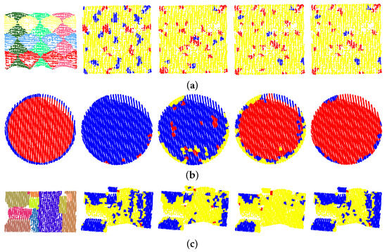
Figure 8.
Comparison of the shape prediction results achieved under different searching scales. (a,b) are the areas marked as Figure 7e,c. (c) is the enlarged area marked as ‘2’ in Figure 6. From left to right: referenced segmentation result; prediction results of fixed neighborhood size: 10, 20, and 30; and our adaptive results. Red: sphere; yellow: cylinder; and blue: planar surface.
4.5. Discussion
In this work, several issues are considered in the segmentation strategy to extract the curved shapes successfully:
- Shape type competition. This issue is unavoidable in complex scenes or when the quality of data is poor. For instance, a horizontal plane may generate more inliers than the cylinders in Figure 8a, causing the poor results seen in Figure 9b. Considering that there are relatively fewer curved shapes, a prediction-then-segmentation strategy that estimates the shape type first is adopted. In Figure 8a, since most points are predicted as cylinders, the influence of other shapes and their meaningless iteration are avoided.
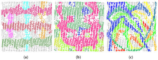 Figure 9. A local comparison of the our direct results with those of efficient RANSAC. (a) Our results before post-segmentation, (b) efficient RANSAC for all shapes, and (c) efficient RANSAC for cylinders only.
 - Spurious shapes. Even if the shape types are successfully identified, spurious shapes will also cause trouble in current methods—i.e., the segmentation results obtained for efficient RANSAC shown in Figure 9c. A spurious plane can be accepted when it contains more inliers or the iteration terminates too early. In our work, the weighted RANSAC approach, which takes the point–shape distance and normal difference into consideration, is adopted. Spurious shapes with greater numbers of points but smaller total weights are suppressed. Moreover, the approaches adopted in post-segmentation and graph-cut-based optimization will also further improve the segmentation results.
- Object scale and neighborhood size. Since the shape prediction approach is achieved through local analysis, it can be influenced by neighborhood size. Meanwhile, when the radius of curved shapes is much larger than the neighborhood size, they can be identified as planes. As such, scale factors are considered in this work, including the radius of curved shapes and the neighborhood size. This ensures the extraction of multiple-scale curved shapes under various different scenes.
5. Conclusions
This paper proposed the use of a robust RANSAC-based segmentation algorithm to detect both planar and curved shapes from dense point clouds. A prediction-then-segmentation strategy was adopted for distinguishing different shape types, in which voxels were used as the basic elements instead of the traditional point-by-point strategy. In shape prediction, multiple-scale neighborhoods were considered; this can be adapted to curved shapes with variable sizes, and multiple shapes such as spheres, cylinders, and cones can be extracted. The point–plane distance, normal difference, and voxel size are all considered as weight terms when evaluating the hypothesis planes using the hybrid voting strategy. The experimental results obtained over both large urban cities and close-range point clouds demonstrate that the proposed methods can outperform the state-of-the-art approach, and the overall completeness and correctness can reach 89% and 88%, respectively.
A limitation of the proposed approach is the extraction of small curved shapes or when the voxels overlap with more than one shape at a smooth segment boundary. Further work will be devoted to speeding up the performance of these methods under denser point clouds and in large scenes as well as the application of this method to more types of shapes and more correct shape boundaries.
Author Contributions
Conceptualization, B.X. and Z.C.; Data curation, Z.C. and S.H.; Formal analysis, X.G. and Y.Z.; Funding acquisition, B.X. and Q.Z.; Investigation, B.X. and S.H.; Methodology, B.X. and Z.C.; Project administration, Q.Z.; Resources, T.L. and D.W.; Software, Z.C.; Supervision, B.X.; Validation, B.X. and Q.Z.; Visualization, Z.C. and Q.Z.; Writing—original draft, B.X. and Z.C.; Writing—review and editing, Q.Z., X.G. and Y.Z. All authors have read and agreed to the published version of the manuscript.
Funding
This work was partly supported by the National Natural Science Foundation of China (Project Nos: 41901408, 41871291, 41871314), the Open Fund of Key Laboratory of Urban Land Resources Monitoring and Simulation, Ministry of Natural Resources (Project No: KF2021-06-015), the Sichuan Science and Technology Program (Project No: 2020YJ0010), the Open Innovative Fund of Marine Environment Guarantee (Grand No: HHB002), as well as the Fundamental Research Funds for the Central Universities (Project No: 2682021CX062).
Data Availability Statement
The ISPRS benchmark data are available at the link below: www.isprs.org/education/benchmarks/UrbanSemLab/Default.aspx (accessed on 6 March 2022). The Stanford 3d Dataset are available at the link below: https://github.com/alexsax/2D-3D-Semantics (accessed on 6 March 2022).
Acknowledgments
The authors acknowledge the provision of the Downtown Toronto dataset by Optech Inc., First Base Solutions Inc., GeoICT Lab at York University, and ISPRS WG III/4.
Conflicts of Interest
The authors declare no conflict of interest.
Abbreviations
The following abbreviations are used in this manuscript:
| RANSAC | RANdom SAmple Consensus |
| MSAC | M-estimate SAmple Consensus |
| MLESAC | Maximum Likelihood-estimate SAmple Consensus |
References
- Haala, N.; Kada, M. An update on automatic 3D building reconstruction. ISPRS J. Photogramm. Remote Sens. 2010, 65, 570–580. [Google Scholar] [CrossRef]
- Musialski, P.; Wonka, P.; Aliaga, D.G.; Wimmer, M.; Van Gool, L.; Purgathofer, W. A survey of urban reconstruction. Comput. Graph. Forum 2013, 32, 146–177. [Google Scholar] [CrossRef]
- Zhu, L.; Lehtomäki, M.; Hyyppä, J.; Puttonen, E.; Krooks, A.; Hyyppä, H. Automated 3D Scene Reconstruction from Open Geospatial Data Sources: Airborne Laser Scanning and a 2D Topographic Database. Remote Sens. 2015, 7, 6710–6740. [Google Scholar] [CrossRef] [Green Version]
- Koelle, M.; Laupheimer, D.; Schmohl, S.; Haala, N.; Rottensteiner, F.; Wegner, J.; Ledoux, H. The Hessigheim 3D (H3D) benchmark on semantic segmentation of high-resolution 3D point clouds and textured meshes from UAV LiDAR and Multi-View-Stereo. ISPRS Open J. Photogramm. Remote Sens. 2021, 1, 100001. [Google Scholar] [CrossRef]
- Zhao, B.; Hua, X.; Yu, K.; Xuan, W.; Chen, X.; Tao, W. Indoor Point Cloud Segmentation Using Iterative Gaussian Mapping and Improved Model Fitting. IEEE Trans. Geosci. Remote Sens. 2020, 58, 7890–7907. [Google Scholar] [CrossRef]
- Shi, W.; Ahmed, W.; Li, N.; Fan, W.; Xiang, H.; Wang, M. Semantic Geometric Modelling of Unstructured Indoor Point Cloud. Int. J. Geo-Inf. 2018, 8, 9. [Google Scholar] [CrossRef] [Green Version]
- Schnabel, R.; Wahl, R.; Klein, R. Efficient RANSAC for Point-Cloud Shape Detection. Comput. Graph. Forum 2007, 26, 214–226. [Google Scholar] [CrossRef]
- Zhu, L.; Kukko, A.; Virtanen, J.-P.; Hyyppä, J.; Kaartinen, H.; Hyyppä, H.; Turppa, T. Multisource Point Clouds, Point Simplification and Surface Reconstruction. Remote Sens. 2019, 11, 2659. [Google Scholar] [CrossRef] [Green Version]
- Lin, Y.; Li, J.; Wang, C.; Chen, Z.; Wang, Z.; Li, J. Fast regularity-constrained plane fitting. ISPRS J. Photogramm. Remote Sens. 2020, 161, 208–217. [Google Scholar] [CrossRef]
- Tian, P.; Hua, X.; Yu, K.; Tao, W. Robust Segmentation of Building Planar Features From Unorganized Point Cloud. IEEE Access 2020, 8, 30873–30884. [Google Scholar] [CrossRef]
- Ying, S.; Xu, G.; Li, C.; Mao, Z. Point Cluster Analysis Using a 3D Voronoi Diagram with Applications in Point Cloud Segmentation. ISPRS Int. J. -Geo-Inf. 2015, 4, 1480–1499. [Google Scholar] [CrossRef]
- Serna, A.; Marcotegui, B.; Hernández, J. Segmentation of Facades from Urban 3D Point Clouds using Geometrical and Morphological Attribute-based Operators. ISPRS Int. J.-Geo-Inf. 2016, 5, 6. [Google Scholar] [CrossRef]
- Li, Y.; Ma, L.; Zhong, Z.; Cao, D.; Li, J. TGNet: Geometric Graph CNN on 3-D Point Cloud Segmentation. IEEE Trans. Geosci. Remote Sens. 2020, 58, 3588–3600. [Google Scholar] [CrossRef]
- Sampath, A.; Shan, J. Segmentation and Reconstruction of Polyhedral Building Roofs From Aerial Lidar Point Clouds. IEEE Trans. Geosci. Remote Sens. 2010, 48, 1554–1567. [Google Scholar] [CrossRef]
- Rabbani, T.; Heuvel, F.V.D.; Vosselman, G. Segmentation of point clouds using smoothness constraints. Int. Arch. Photogramm. Remote Sens. Spat. Inf. Sci. 2006, 36, 248–253. [Google Scholar]
- Luo, N.; Jiang, Y.; Wang, Q. Supervoxel Based Region Growing Segmentation for Point Cloud Data. Int. J. Pattern Recognit. Artif. Intell. 2020, 35, 2154007. [Google Scholar] [CrossRef]
- Wang, X.; Liu, S.; Shen, X.; Shen, C.; Jia, J. Associatively Segmenting Instances and Semantics in Point Clouds. arXiv 2019, arXiv:1902.09852. [Google Scholar]
- Zhao, L.; Tao, W. JSNet: Joint Instance and Semantic Segmentation of 3D Point Clouds. arXiv 2019, arXiv:1912.09654. [Google Scholar] [CrossRef]
- Xu, B.; Jiang, W.; Shan, J.; Zhang, J.; Li, L. Investigation on the Weighted RANSAC Approaches for Building Roof Plane Segmentation from LiDAR Point Clouds. Remote Sens. 2016, 8, 5. [Google Scholar] [CrossRef] [Green Version]
- Fischler, M.A.; Bolles, R.C. Random sample consensus: A paradigm for model fitting with applications to image analysis and automated cartography. Commun. ACM 1981, 24, 381–395. [Google Scholar] [CrossRef]
- Choi, S.; Kim, T.; Yu, W. Performance Evaluation of RANSAC Family. In Proceedings of the British Machine Vision Conference, London, UK, 7–10 September 2009; pp. 81.1–81.12. [Google Scholar]
- Chen, D.; Zhang, L.Q.; Li, J.; Liu, R. Urban building roof segmentation from airborne lidar point clouds. Int. J. Remote Sens. 2012, 33, 6497–6515. [Google Scholar] [CrossRef]
- Frederic, B.; Michel, R. Hybrid image segmentation using LiDAR 3D planar primitives. In Proceedings of the Workshop “Laser scanning 2005”, Enschede, The Netherlands, 12–14 September 2005. [Google Scholar]
- Awwad, T.M.; Zhu, Q.; Du, Z.; Zhang, Y. An improved segmentation approach for planar surfaces from unconstructed 3D point clouds. Photogramm. Rec. 2010, 25, 5–23. [Google Scholar] [CrossRef]
- Zeineldin, R.A.; El-Fishawy, N.A. FRANSAC: Fast RANdom Sample Consensus for 3D Plane Segmentation. Int. J. Comput. Appl. 2017, 167, 30–36. [Google Scholar]
- Papon, J.; Abramov, A.; Schoeler, M.; Wörgötter, F. Voxel Cloud Connectivity Segmentation-Supervoxels for Point Clouds. In Proceedings of the 2013 IEEE Conference on Computer Vision and Pattern Recognition, Portland, OR, USA, 23–28 June 2013; pp. 2027–2034. [Google Scholar]
- Torr, P.H.; Zisserman, A. MLESAC: A new robust estimator with application to estimating image geometry. Comput. Vis. Image Underst. 2000, 78, 138–156. [Google Scholar] [CrossRef] [Green Version]
- Berkhin, P. Survey of Clustering Data Mining Techniques; Springer: New York, NY, USA, 2006. [Google Scholar]
- Gallo, O.; Manduchi, R.; Rafii, A. CC-RANSAC: Fitting planes in the presence of multiple surfaces in range data. Pattern Recognit. Lett. 2011, 32, 403–410. [Google Scholar] [CrossRef] [Green Version]
- Lin, Y.; Wang, C.; Zhai, D.; Li, W.; Li, J. Toward better boundary preserved supervoxel segmentation for 3D point clouds. ISPRS J. Photogramm. Remote Sens. 2018, 143, 39–47. [Google Scholar] [CrossRef]
- Xu, Y.; Tong, X.; Stilla, U. Voxel-based representation of 3D point clouds: Methods, applications, and its potential use in the construction industry. Autom. Constr. 2021, 126, 103675. [Google Scholar] [CrossRef]
- Achanta, R.; Shaji, A.; Smith, K.; Lucchi, A.; Fua, P.; Süsstrunk, S. SLIC Superpixels Compared to State-of-the-Art Superpixel Methods. IEEE Trans. Pattern Anal. Mach. Intell. 2012, 34, 2274–2282. [Google Scholar] [CrossRef] [Green Version]
- Wang, N.; Chen, F.; Yu, B.; Wang, L. A Strategy of Parallel SLIC Superpixels for Handling Large-Scale Images over Apache Spark. Remote Sens. 2022, 14, 1568. [Google Scholar] [CrossRef]
- Comaniciu, D.; Meer, P. Mean shift: A robust approach toward feature space analysis. IEEE Trans. Pattern Anal. Mach. Intell. 2002, 24, 603–619. [Google Scholar] [CrossRef] [Green Version]
- Zhou, Y.; Ju, L.; Wang, S. Multiscale Superpixels and Supervoxels Based on Hierarchical Edge-Weighted Centroidal Voronoi Tessellation. IEEE Trans. Image Process. 2015, 24, 3834–3845. [Google Scholar] [CrossRef] [PubMed]
- Xu, Y.; Tuttas, S.; Hoegner, L.; Stilla, U. Geometric Primitive Extraction from Point Clouds of Construction Sites Using VGS. IEEE Geosci. Remote Sens. Lett. 2017, 14, 424–428. [Google Scholar] [CrossRef]
- Song, S.; Lee, H.; Jo, S. Boundary-enhanced supervoxel segmentation for sparse outdoor LiDAR data. Electron. Lett. 2014, 50, 1917–1919. [Google Scholar] [CrossRef] [Green Version]
- Shen, J.; Hu, M.; Yuan, B. A robust method for estimating the fundamental matrix. In Proceedings of the 6th International Conference on Signal Processing, Beijing, China, 26–30 August 2002; Volume 1, pp. 892–895. [Google Scholar]
- Moisan, L.; Moulon, P.; Monasse, P. Fundamental Matrix of a Stereo Pair, with A Contrario Elimination of Outliers. Image Process. Line 2016, 6, 89–113. [Google Scholar] [CrossRef] [Green Version]
- Su, Z.; Gao, Z.; Zhou, G.; Li, S.; Song, L.; Lu, X.; Kang, N. Building Plane Segmentation Based on Point Clouds. Remote Sens. 2021, 14, 95. [Google Scholar] [CrossRef]
- Li, L.; Yang, F.; Zhu, H.; Li, D.; Li, Y.; Tang, L. An improved RANSAC for 3D point cloud plane segmentation based on normal distribution transformation cells. Remote Sens. 2017, 9, 433. [Google Scholar] [CrossRef] [Green Version]
- Yan, J.X.; Shan, J.; Jiang, W.S. A global optimization approach to roof segmentation from airborne lidar point clouds. ISPRS J. Photogramm. Remote Sens. 2014, 94, 183–193. [Google Scholar] [CrossRef]
- Dong, Z.; Yang, B.; Hu, P.; Scherer, S. An efficient global energy optimization approach for robust 3D plane segmentation of point clouds. ISPRS J. Photogramm. Remote Sens. 2018, 137, 112–133. [Google Scholar] [CrossRef]
- Rottensteiner, F.; Sohn, G.; Gerke, M.; Wegner, J.D.; Breitkopf, U.; Jung, J. Results of the ISPRS benchmark on urban object detection and 3D building reconstruction. ISPRS J. Photogramm. Remote Sens. 2014, 93, 256–271. [Google Scholar] [CrossRef]
- Armeni, I.; Sax, S.; Zamir, A.R.; Savarese, S. Joint 2d-3d-semantic data for indoor scene understanding. arXiv 2017, arXiv:1702.01105. [Google Scholar]
- Awrangjeb, M.; Fraser, C.S. An Automatic and Threshold-Free Performance Evaluation System for Building Extraction Techniques From Airborne LIDAR Data. IEEE J. Sel. Top. Appl. Earth Obs. Remote Sens. 2014, 7, 4184–4198. [Google Scholar] [CrossRef]
Publisher’s Note: MDPI stays neutral with regard to jurisdictional claims in published maps and institutional affiliations. |
© 2022 by the authors. Licensee MDPI, Basel, Switzerland. This article is an open access article distributed under the terms and conditions of the Creative Commons Attribution (CC BY) license (https://creativecommons.org/licenses/by/4.0/).