GBB-Nadir and KLIMA: Two Full Physics Codes for the Computation of the Infrared Spectrum of the Planetary Radiation Escaping to Space

Abstract

In 2019 the Far-Infrared Outgoing Radiation Understanding and Monitoring (FORUM) mission was selected to be the 9th Earth Explorer mission of the European Space Agency (ESA). In the preparatory phase of the mission there was the need for accurate and versatile codes to compute the spectrally resolved Earth radiation escaping to space ( outgoing long-wave radiation, OLR), targets for the FORUM measurements.Moreover, for the study of planetary atmospheres, several instruments measuring the planetary radiation escaping to space have been deployed (i.e., the planetary Fourier spectrometer on Mars express or composite infrared spectrometer on Cassini). For both the analysis of the measurements of these instruments and the design of new instruments, reliable radiative transfer codes need to be available. In this paper, we describe two full physics codes, Geofit broadband-Nadir (GBB-Nadir) and Kyoto protocol-informed management of adaptation (KLIMA), both able to compute the OLR spectrum, while GBB-Nadir is only a forward model, and therefore computes the spectra only, KLIMA implements the computation of spectral radiance derivatives with respect to atmospheric parameters and therefore it is suitable to be used in retrieval codes. The GBB-Nadir code can be interfaced with radiative transfer solvers that include representations of multiple scatterings, making it suitable to compute the radiances in all-sky conditions. KLIMA has been extensively validated comparing its radiances to ones generated by the widely used line-by-line radiative transfer model (LBLRTM) code. In this paper, we describe the latest version of both codes and their comparison. We compared the optical depth computed by GBB-Nadir and KLIMA for given values of pressure, temperature and gas columns for most gases active in the far-infrared and thermal-infrared spectral regions. We show that the optical depths computed by the two codes are in very good agreement. We compared the simulated spectra in clear sky conditions for three different atmospheres (equatorial, mid-latitude and polar) at resolutions of the FORUM instrument. The differences found are well below the expected noise of the FORUM instrument. The KLIMA code has already been used to simulate the observations of the Mars atmosphere, while the limb version of the GBB code has been used to simulate the radiances measured in the limb geometry of planetary atmospheres (Titan and Jupiter). Therefore, we may safely affirm that both codes can be used to simulate the nadir measurements of planetary atmospheres.

1. Introduction

The thermal emission of the Earth and the atmosphere system escaping to space is called outgoing long-wave radiation (OLR). Its spectrum mainly covers two wide sub-ranges of the infrared radiation, namely, the medium or thermal infrared (MIR or TIR, from 667 to 2500 cm${}^{-1}$ and from 15 to 4 μm wavelength, respectively) and the far infrared (FIR, from 100 to 667 cm${}^{-1}$ and from 100 to 15 μm wavelength). The OLR is a critical regulator of the terrestrial radiative balance, and it is strongly sensitive to the surface emissivity, cloud coverage and various absorbing species in the FIR and TIR spectral regions. In particular, the FIR spectral region is strongly sensitive to mid-upper-level tropospheric humidity, that produces a peak in the cooling rate of the atmosphere [1,2]. The most important green house gas, CO${}_2$, has its strongest absorption band across the FIR and TIR spectral regions (from $\sim 500$ to $\sim 800$ cm${}^{-1}$) and other important molecules such as O${}_3$, N${}_2$O, and HNO${}_3$ have pure rotational or vibro-rotational transitions in the FIR and TIR spectral regions. Moreover, in the OLR spectrum many important signatures are present, signatures that enable the study of various phenomena driving the Earth climate. An example is cirrus clouds, that are essential in determining the Earth’s energy budget [3,4]. They may have both warming and cooling effects and their relative importance depends on the cloud’s optical and micro-physical properties [5,6,7,8].

To date, space missions have only sampled part of the Earth’s OLR spectral range (only extending up to 25 μm), and only a few spectral measurements have been collected in the FIR region [3,9,10]. Conversely, its has been a long time since planetary atmospheres have been observed in the FIR and TIR spectral regions. For example, the Martian atmosphere is and has been measured by the planetary Fourier spectrometer (PFS), on board Mars express (MEx) [11] with a channel covering the FIR and TIR spectral regions. Another example is the composite infrared spectrometer (CIRS) on Cassini [12] that has observed Saturn and its moons in the FIR and TIR spectral regions from 2004 to 2017.

To provide the entire spectrum of the Earth’s OLR, the Far-Infrared Outgoing Radiation Understanding and Monitoring (FORUM) mission [13] was proposed and selected in September 2019 to be the Earth Explorer 9 (EE9) mission of the European Space Agency (ESA). FORUM will deliver an improved understanding of the climate system by supplying for the first time, in conjunction with the measurements provided by the infrared atmospheric sounding instrument-next generation (IASI-NG) instrument (flying on board the Meteorological Operational Satellite, Second Generation (Metop SG)), a complete spectral characterisation of the Earth’s OLR. FORUM will measure the outgoing thermal radiation between 100 and 1600 cm${}^{-1}$, at 0.5 cm${}^{-1}$ spectral resolution, while IASI-NG will supply the OLR in the spectral range 645 and 2760 cm${}^{-1}$. In this way, FORUM together with IASI-NG, will deliver a truly unique dataset of the Earth’s entire emission spectrum from 100 to 2760 cm${}^{-1}$ (from $3.62$ to 100 μm in wavelength) that will help the scientific community understand links between crucial underlying physical processes driving climate change, their spectral signatures, the greenhouse effect, and the overall Earth radiation budget [14].

Designing a forward model to describe the instrument and the physics of the measurement is one of the fundamental parts in the exploitation of satellite OLR measurements (i.e., solving an atmospheric retrieval problem, assimilate the measured radiances in weather forecasting models and/or perform the preparatory studies for the development of satellite missions such as FORUM). The codes that compute the OLR spectrum starting from the spectroscopic parameters and implement a thorough representation of the physics which the radiative transfer is based on are called full physics codes. Examples of full physics codes used to simulate the OLR are: the line-by-line radiative transfer model (LBLRTM) code [15], widely used to simulate the spectrum at the top of the Earth’s atmosphere, and the atmospheric radiative transfer for Titan (ARTT) for Titan’s atmosphere [16,17]. Usually, running a full physics model is very time-consuming. To overcome this problem fast codes simulating the measured spectra have been developed. For example, the $\sigma$-IASI code ([18], and references therein) is a fast code developed for the simulation and analysis of the IASI measurements, which, given their enormous number, could not be handled by a full physics code. Another example is the radiative transfer for TOVS (RTTOV) code [19], commonly used by meteorological and climate models to both assimilate the radiances measured by different satellites and to compare the outputs of the models with observations. For planetary atmospheres we cite the code developed by Ignatiev et al. [20] for the analysis of the PFS measurements. To speed up the computation time, fast codes make use of several approximations. These approximations should be validated through comparisons with the outputs of full physics radiative transfer codes. The Geofit broadband nadir (GBB-Nadir) code and the Kyoto protocol-informed management of the adaptation (KLIMA) code, described in this paper, are two of these codes. GBB-Nadir was initially designed to simulate the spectra recorded by the along-track scanning radiometer (ATSR) instrument series [21,22], and therefore optimised for the computation in a smaller spectral range than the one covered by FORUM or IASI-NG. In particular, the strong CO${}_2$ band at 700 cm${}^{-1}$ and the FIR part of the spectrum were not covered. Moreover, the only scattering properties used in the code were the ones of cloud particles approximated as spheres of both water and ice. The KLIMA code was originally designed to analyse IASI spectra and retrieve the CO${}_2$ vertical concentration [23]; therefore, it only covered the TIR spectral region. Over the years KLIMA has been extensively validated against the spectra simulated with the widely recognised LBLRTM code [15].

This paper describes the latest versions of the GBB-Nadir and KLIMA codes, both updated during an Italian Space Agency (ASI) project (FORUM–Scienza) connected to the FORUM mission, and the extensive inter-comparison exercise both for single gas optical depths and spectra performed within the project. Because of the focus of the project, all the inter-comparisons reported here refer to the expected spectral resolution (0.5 cm${}^{-1}$) and noise equivalent spectral radiance (NESR) of the FORUM mission. The paper is organized as follows: Section 2 is dedicated to the GBB-Nadir code, with a thorough description of the various implementation strategies (some of which are similar to the KLIMA code). Section 3 describes the KLIMA code, while Section 4 reports the results of the inter-comparison tests between GBB-Nadir and KLIMA. Finally, Section 5 discusses the conclusions of the work.

2. The GBB-Nadir Code

The GBB-Nadir code is a stand-alone forward model (FM) that can simulate high-resolution top of atmosphere (TOA) radiance using a line-by-line calculation of the absorption properties of a stratified and plane-parallel atmosphere. The GBB-Nadir code is the nadir version of the GBB code. The original GBB code was the broadband version of the Geofit FM [24], developed for the simulation of the limb TIR measurements of the Michelson interferometer for passive atmospheric sounding (MIPAS) instrument on ENVISAT, and included a line-by-line computation of the absorption cross-sections of the atmospheric gases similar to the one developed by Ridolfi et al. [25]. The geometrical part of the code was modified in the frame of the ATSR long-term stability (ALTS) project, funded by ESA, to allow simulations of spectra acquired by a Nadir-looking instrument (ATSR), as reported by [21,22]. In the frame of the FORUM–Scienza project, funded by the ASI, the GBB code was extensively modified to become the GBB-Nadir code described in this paper.

For each atmospheric layer, the GBB-Nadir code stores the optical depths, both the gaseous absorption and clouds or aerosols, and the scattering properties, such as the single scattering albedo and the scattering phase function, in external files. In the second step GBB-Nadir solves the radiative transfer equation (RTE) for a user-defined number of viewing geometries targeting the Earth’s surface, making use of an internal radiative transfer routine described in this paper and used for clear sky simulations. Alternatively, GBB-Nadir solvesdiscrete ordinate radiative transfer (DISORT) [26] or linearized discrete ordinate radiative transfer (LIDORT) [27] RTE in cases where multiple scattering has to be taken into account. Convolutions with any instrumental response function or field of view function have to be performed in a separate step.

GBB-Nadir can be interfaced with any spectroscopic database. In fact, the spectroscopic data used in simulations of the atmospheric spectra are processed by a separate code that reads the chosen spectroscopic databases, selects the data to be used and writes them in the appropriate format used by the GBB-Nadir code. Each molecule has an internally assigned code, similar to the codes used in the HITRAN (high-resolution transmission) database [28]. The transitions are chosen according to their intensity at the average atmospheric temperature and expected atmospheric gas concentration to be simulated.

Scattering bodies such as aerosol particles or cloud particles can be added to the modelled atmosphere, and GBB-Nadir will compute their scattering properties. The scattering particles can be spherical or non-spherical. In the former case, their single scattering properties (scattering and extinction coefficients and Legendre polynomial coefficients approximating their scattering phase function) can be computed starting from the refractive index. These can be provided as a function of the frequency or wavelength using the Lorentz–Mie theory, implemented by the code developed by Mishchenko [29], for the scattering of light by poly-disperse homogeneous spherical particles. For non-spherical particles, the GBB-Nadir code reads external files containing pre-computed single scattering properties. The handling of non local thermodynamic equilibrium is not implemented in the GBB-Nadir code, because its effect is negligible in Nadir-viewing geometries.

2.1. The Main Body of the GBB-Nadir Code

GBB-Nadir computes the high-resolution radiances in the required spectral region dividing it into 5 cm${}^{-1}$ wide contiguous spectral regions, called micro-windows (MW), overlapped over a 0.1 cm${}^{-1}$ wide interval. For each MW, spectroscopic data are provided in separate files, using the code mentioned in the previous section. For heavy molecules, for which spectroscopic properties are provided as tabulated cross-sections, the code directly reads the database files distributed by the developers. The spectral grid at the optical depths and the radiance to be computed can be selected by the user. The two grids can be coincident or the radiance can be computed from a grid that is a multiple of the one used to compute the optical depths. The vertical distribution of the temperature, pressure and volume mixing ratio (VMR) of the atmospheric gases are selected by the user among an internally provided database or using external files. The code computes the atmospheric vertical layering starting from a set of altitude levels provided by the user and from the lowest and topmost altitudes, again decided by the user. The code automatically inserts additional altitude levels if the temperature difference between two adjacent points is larger than a user-defined threshold. The user can also skip all these controls and use the vertical levels only at which the atmospheric input profiles are provided.

Surface emissivity is read from an external file, interpolated onto the internal spectral grid, and then transformed into reflectivity assuming no transmission below the surface. The interpolation of the atmospheric quantities on the used atmospheric vertical grid is linear for temperature and exponential for pressure. For the VMRs, the user can choose between linear or exponential interpolation. If no requirement is made, the default value is to use linear interpolation for all the VMRs.

After interpolating the atmospheric profiles on the required vertical grid and acquiring and storing the needed spectroscopic parameters, GBB-Nadir computes the atmospheric status relative to each layer using the Curtis–Godson integrals [30,31]. Then the actual calculation of the absorption cross-sections on the required spectral grid for each spectral layer is performed.

2.1.1. Absorption Cross-Section Calculation

The contribution of a single absorption line to the absorption cross-section of the gaseous species m in the layer l at wave number $\sigma$ can be represented by the product of the line strength at the equivalent temperature T of the atmospheric layer $S\left(T\right)$ and the wave number-dependent line shape function as follows:

$$K(\sigma ,p,T)=S\left(T\right)L(\sigma ,p,T)$$

(1)

where K is the single line cross-section at the frequency $\sigma$, pressure p and temperature T, and $L(\sigma ,p,T)$ is the line shape. Precisely, the line strength is temperature-dependent, and the line shape depends on the layer temperature and pressure. The line strength is corrected for the temperature of the layer using the expression given in [32] using the latest version of the total internal partition function (TIP) of [33]. If, for a molecular species, the TIP-tabulated coefficients are not available, the line strength is scaled with the ratio between the layer temperature and the reference temperature elevated to the power of 1.5. The central frequency of the absorption line is computed taking into account the frequency shift due to pressure effects.

The broadening of the absorption lines in the atmosphere is mainly due to collisions among molecules (linked to pressure) and the Doppler effect due to the absorbing molecules thermal velocity (linked to temperature). The Lorentzian function typically represents the line shape due to the pressure broadening, while the line shape due to the thermal motion can be represented by a Gaussian distribution of width equal to the Doppler broadening. While the Doppler broadening can be computed simply using the molecular mass and temperature of the atmospheric layer, the pressure broadening is usually obtained by combining the tabulated self and foreign broadening coefficients, weighting them according to the atmospheric gas abundance and scaling the result for the correct pressure and temperature.

In general, the final line shape is a combination of the shape resulting from both the Doppler and pressure broadening, which can be represented by the Voigt function, a convolution between the Doppler and Lorentz line shapes. The convolution integral of the Voigt line shape is very time-consuming; therefore, the GBB-Nadir code implements the Voigt function with the rational approximation (with a relative accuracy of ${10}^{-4}$) introduced by Humlicek [34]. In order to speed up the computation, the line shape is computed with the Lorentz function and the Voigt line shape is only used in the region close to the line centre, where the difference between the Voigt and Lorentz line shapes is relatively large. The frequency region where the Voigt function is used is automatically decided according to the value of the Doppler and Lorentz widths of the considered transition. The line shape is estimated for each line whose frequency is within an interval of ±25 cm${}^{-1}$ from the considered spectral point unless its contribution to the cross-section is lower than a fixed threshold (typically 10${}^{-30}$ cm${}^2$/molecule). Moreover, for computational efficiency, the line shape is calculated in two different regions using different spectral grids (that may not coincide with the user-required spectral grid), finer close to the central line and coarser elsewhere. At the end of the computation, the line shape is linearly interpolated onto the spectral grid required by the user.

For the correct modelling of water vapour absorption and emission, GBB-Nadir implements the water vapour continuum parameterisation MT_CKD (Mlawer Tobin_Clough Kneizys Davies url: http://rtweb.aer.com/continuum_description.html, accessed on 23 March 2023) accounting for the cumulative effects of neglecting the weakest H${}_2$O lines and the representation of the collision-induced absorption. Different versions of the MT_CKD model (v2.5 to v4.1) are available, with most included in the GBB-Nadir code, and can be chosen by the user. Code in the continuum models for N${}_2$, O${}_2$, O${}_3$ and CO${}_2$ are also implemented. The use of each molecular continuum model can be decided by the user.

The line-mixing effect produces a distortion of the observed line shape and is mainly observed for CO${}_2$ in spectral regions with dense rotational or vibration–rotation bands. This effect can be reproduced using a modified Voigt line shape, called the speed-dependent Voigt (SDV) line shape or performing a full line mixing treatment (FLM).

The HITRAN database distributes a code to reproduce the line mixing effect that applies the treatment developed by [35] to compute either the FLM or the broadening coefficients to be used in the SDV approximation. It should be noted that the FLM is very time-consuming and increases the computing time by a factor of 26. The SDV is computationally more efficient but in some spectral regions it produces negative cross-sections; therefore, it should be used with some precautions. The spectroscopic database linked to LBLRTM [15] (AER url: http://rtweb.aer.com/line_param_frame.html, accessed on 23 March 2023) directly provides the broadening coefficients to be used in the SDV approximation; therefore, it is the fastest way to reproduce the CO${}_2$ line mixing. The team also developed a continuum model that avoids the negative cross-sections produced by the HITRAN SDV distribution. In the GBB-Nadir code, the option to compute the line mixing with the HITRAN code or LBLRTM approach is implemented. In the latter case, the CO${}_2$ AER spectroscopic data and CO${}_2$ continuum model released by the LBLRTM team are used (and substituted in for the original CO${}_2$ spectroscopic data read in the provided spectroscopic files). Figure 1 shows the radiances computed with GBB-Nadir for polar (light-blue), mid-latitude (green) and tropical (purple) atmospheres without the LM treatment. The three lower panels of the same figure (Figure 1) show the differences in the FORUM spectral region between the spectra simulated with the three approaches described above the spectra shown in the top panel, computed without the LM treatment. The first two panels show the differences in the HITRAN LM case (top panel FLM and central panel SDV). The bottom panel of Figure 1 shows the differences between the simulations with the LBLRTM approach for LM using the AER v3.8 spectroscopic dataset instead of HITRAN2020 as in the cases shown in the other two panels of the same figure. We see that both the HITRAN FLM and the LBLRTM approach produce very similar results. The HITRAN SDV approach produces large differences in the CO${}_2$ spectral region, much larger than the FLM approach, that can be ascribed to the negative cross-sections it sometimes produces.

The tabulated cross-sections in the various spectroscopic databases for complex molecular species for which line-by-line data are unavailable contain data on the molecular absorption for sparse pressure and temperature (p, T) pairs. In order to obtain accurate cross-sections for the (p, T) values of the layer, the code performs a two-dimensional interpolation using a triangulation approach. When only one (p, T) pair is present, the tabulated cross-sections are scaled with the reference temperature and required temperature ratio at the power of 1.5.

2.1.2. Calculation of the Optical Depth of Each Atmospheric Layer

The optical depth is a quantity that describes how much absorption occurs when the radiation travels through an absorbing medium, such as the atmosphere of a star or planet, before it is absorbed or scattered. A completely transparent medium has an optical depth of zero. A medium with a low optical depth is described as optically thin, whereas one with a high optical depth is optically thick. Absorption and scattering vary with wavelength or frequency, so the optical depth has to be computed for a particular wavelength or frequency. The optical depth $\tau$ of a generic atmospheric layer l (comprised between the altitudes z and $z+∆z$) at wave number $\sigma$ is given by the following formula:

$$\tau (\sigma ,l)=(\sum _{m=1}^{N}K(\sigma ,l,m)X_{l,m})\eta ∆z$$

(2)

where $K(\sigma ,l,m)$ and $X_{l,m}$ are the gaseous cross-section and the volume mixing ratio of species m and layer l, respectively, $\eta$ is the atmospheric layer number density and $∆z$ is the optical path along with the radiation travels within layer l.

To avoid discontinuities in the final spectrum, the MWs are defined in slightly overlapping spectral regions. The optical depths computed in the overlapping frequency regions are saved and combined with the values computed in the subsequent one throughout a weighted linear interpolation. The optical depths for each layer are then sequentially written in an output file specified by the user. This strategy enables the computation of the optical depths to be skipped if we want to repeat the simulations using the same atmospheric status with different scattering bodies or RTE solvers.

2.2. Scattering Properties

If the contribution to the spectrum of scattering bodies has to be included, the GBB-Nadir code performs all the computations needed to include it in the simulated spectrum. As a first step the vertical profiles of the particle density and effective radii for each type of scattering particle (i.e., ice, water, aerosols) are read. Then the scattering properties of the particles (Legendre polynomial coefficients, extinction and scattering coefficients) are either internally calculated or read from look-up tables (LUTs). In the case of more than one particle type, the properties are computed for each kind of scatter and then weighted using the relative abundance of the particles to obtain a single set of scattering properties for each atmospheric layer.

When internally calculated, the scattering properties are computed starting from the real and imaginary part of the refractive index of the considered particles (provided by the user) applying the Mie scattering theory for spherical particles implemented in the Mishchenko subroutine [29] on a coarse frequency grid (one point any 5 cm${}^{-1}$) and then interpolated with a second-degree polynomial to the frequency grid required by the user. Alternatively, the single scattering properties of each type of particle can be provided in one or more external files. GBB-Nadir can cope with different size distributions of the same particle type for different atmospheric layers. The tabulated properties are interpolated for the required spectral grid with the same interpolation method used for spherical particles. Then, the optical depths due to the scattering particles are added to the pre-computed clear sky optical depths and stored in a new file. The scattering albedo and the Legendre polynomial coefficients used to represent the scattering phase functions are stored in a separate file.

2.3. Radiative Transfer Solver

Once the final total optical depths of each atmospheric layer (and the scattering properties if required) are computed and stored, GBB-Nadir performs the actual radiative transfer to compute the spectrally resolved radiance escaping to space. The radiance is a function of both the vertical distribution of the temperature and the atmospheric gases included in the optical depths computation. For the sake of simplicity in this section, all the temperature and composition dependencies in the reported formulas are omitted. The radiative transfer can be performed either with the DISORT method (directly implemented in the GBB-Nadir code) or with the internal radiative transfer equation (RTE) solver described in this section. The latter can only be exploited when clear sky simulations are required, while the DISORT RTE solver can be used in all sky conditions. If other RTE solvers are used (e.g., LIDORT) a different code is required, that reads the files computed by GBB-Nadir and translates them into the format required by the chosen RTE solver.

The internal RTE solver implements the following equation for the evaluation of the TOA signal S at each single frequency point $\sigma$:

$$\begin{array}{ccc}\hfill S\left(\sigma \right)& =& \epsilon \left(\sigma \right)B\left(T_s\right)T{r}_{TOT}^{\prime }+R\left(\epsilon \left(\sigma \right)\right)+\hfill \\ & & {\int }_0^{z_{TOP}}B\left(T\left(z\right)\right)(1-e^{-{\tau }^{\prime }(\sigma ,z)})T{r}^{\prime }(z,z_{TOP})dz\hfill \end{array}$$

(3)

with

$$\begin{array}{ccc}\hfill T{r}_{TOT}^{\prime }& =& {\left(T{r}_{TOT}\right)}^{\mu }\hfill \end{array}$$

(4)

$$\begin{array}{ccc}\hfill T{r}^{\prime }(z,z_{TOP})& =& {\left(Tr(z,z_{TOP})\right)}^{\mu }\hfill \end{array}$$

(5)

$$\begin{array}{ccc}\hfill {\tau }^{\prime }(\sigma ,z)& =& \tau (\sigma ,z)\mu \hfill \end{array}$$

(6)

where

• $B\left(T_s\right)$ and $B\left(T\right(z\left)\right)$ are the Planck functions at temperature $T_s$ at the surface and $T\left(z\right)$ at the layer at altitude z representing the thermal emission of the surface and source function of the atmospheric layer;
• $\epsilon \left(\sigma \right)$ is the surface emissivity;
• $\tau (\sigma ,z)$ is the optical depth of the layer at altitude z;
• $Tr(z,z_{TOP})$ is the transmittance of the atmosphere from z up to the top of the atmosphere ($z_{TOP}$);
• $T{r}_{TOT}$ is the total transmittance of the atmospheric column along the vertical direction;
• $\mu =1/cos\left(\theta \right)$ is the so-called airmass factor, with $\theta$ as the angle between the viewing geometry and the vertical direction;
• $R\left(\epsilon \right(\sigma \left)\right)$ is the atmospheric thermal radiation emitted downwards that reaches the surface in the point intercepted by the line of sight (LOS), reflected back towards the observer and attenuated by the atmosphere along the optical path.

Considering a Lambertian surface albedo, $R\left(\epsilon \right(\sigma \left)\right)$ is computed as:

$$R\left(\epsilon \left(\sigma \right)\right)=T{r}_{TOT}^{\prime }\frac{1-\epsilon \left(\sigma \right)}{\pi }{\int }_0^{2\pi }d\varphi {\int }_{z_{TOP}}^{0}dz{\int }_0^{1}cos\left(\theta \right)dcos\left(\theta \right)B\left(T\left(z\right)\right)(1-e^{-{\tau }^{\prime }(\sigma ,z)})T{r}^{\prime }(z,z_0)$$

(7)

where $T{r}^{\prime }(z,z_0)$ is the transmittance of the slant atmospheric column from the level at altitude z down to the surface. Precisely, the integral over the vertical coordinate, the zenith and azimuth angles represent the total downward atmospheric emission reaching the observed point on the surface. The integration on the azimuth is just a multiplicative factor, since the modelled atmosphere is assumed horizontally homogeneous. In Equation (7) $\pi$ is not a dimensionless number but has the dimension of an angle (radiants). Obviously, in the implementation of Equations (3) and (7) in the GBB-Nadir code the integrals are replaced by a summation and the values that refer to the altitudes are replaced by the Curtis–Godson equivalents of the layers. The measurement unit of the resulting spectral radiance $S\left(\sigma \right)$ depends upon the unit used to express the Planck function B. Usually the spectral radiance is expressed in nW/ (sr cm${}^{-1}$ cm${}^2$) or W/ (sr cm${}^{-1}$ m${}^2$).

Because we assume the atmosphere in local thermodynamic equilibrium, $B\left(T\right(z\left)\right)$ represents the source function at the temperature of the layer of average altitude z; however, when the layer’s optical depth is very large (larger than the threshold value of ${10}^{-6}$), the source function is corrected considering both the layer’s optical depth and the Plank function at temperatures at the borders of the considered atmospheric layer using the following expression (see Equation (13) of [36]):

$$B^{\prime }\left(T\left(z\right)\right)=B\left(T_{up}\right)+2[B\left(T\left(z\right)\right)-B\left(T_{up}\right)][\frac{1}{\tau (\sigma ,z)}-\frac{e^{-\tau (\sigma ,z)}}{1-e^{-\tau (\sigma ,z)}}]$$

(8)

where $B\left(T_{up}\right)$ is the black body emission at the temperature of the upper boundary of the layer ($T_{up}$). Therefore, the more optically thick the layer is, the more $B^{\prime }\left(T\left(z\right)\right)$ converges to $B\left(T_{up}\right)$. The same equation is applied to the downward-emitted radiation, substituting $T_{up}$ with the temperature of the bottom layer ($T_{dn}$), with the emissions approaching the black body emission $B\left(T_{dn}\right)$ of the lower boundary of the layer for high values of $\tau (\sigma ,z)$.

This weighting is also applied in the radiative transfer codes KLIMA, described in Section 3, LBLRTM [36], DISORT [26] and LIDORT [27]. Figure 2 shows a comparisons of the radiances obtained using the internal radiative transfer and the DISORT solver on the same optical depths, for the FORUM spectral region and at the FORUM resolution. The major differences (shown by the purple line in Figure 2) are due to the fact that DISORT makes use of a series expansions of the Plank function $B\left(T\right(z\left)\right)$, while in the internal radiative transfer we use the exact expression. When the exact Plank expression is substituted with the same series expansions used by the DISORT solver, the differences approach zero, as shown by the green line in Figure 2. In any case the differences are within 1/10 of the FORUM goal noise.

3. The KLIMA Code

The KLIMA code is a self-standing algorithm, developed in FORTRAN, able to both simulate and analyse the atmospheric spectral radiance acquired by remote sensing measurements in clear sky conditions. KLIMA is an extension of a previous code called MARC (millimetre-wave atmospheric-retrieval code) [37] specifically developed for the millimetre-wave spectral region and limb geometry. The updated version of this code, KLIMA, can be used in various geometrical configurations (limb [38,39], zenith [40] and nadir [23,41,42,43,44]) and spectral bands (from millimetre and sub-millimetre wave [37] to near-infrared [45]). Finally, the KLIMA code was also used to simulate the nadir and limb radiances for a Martian atmosphere in the context of some internal tests related to the planetary Fourier spectrometer (PFS) instrument on board of Mars express (MEx) [11] and compared with the simulations obtained using the code described by Ignatiev et al. [20].

A summary of the instruments whose measurements can be simulated by the KLIMA code is reported in

Table 1. List of instruments simulated with the KLIMA code. The table reports the name of the instrument, the viewing geometry, and the spectral band.

Instrument or Mission	Band	Geometry
MARSCHALS [37]	290–350 GHz	Limb
REFIR-PAD [41]	100–1000 cm${}^{-1}$	Nadir
PFS-MEx	200–9000 cm${}^{-1}$	Limb/Nadir
FLEX [45]	0.7 μm	Nadir
IASI [23]	645–2760 cm${}^{-1}$	Nadir
IASI-NG [43]	645–2760 cm${}^{-1}$	Nadir
FORUM [44]	100–1600 cm${}^{-1}$	Nadir
FIRMOS [40]	100–1600 cm${}^{-1}$	Zenith
FIRMOS-B [46]	100–1600 cm${}^{-1}$	Nadir/Zenith

. Moreover, KLIMA can simultaneously simulate and analyse the observations of two or more instruments [46].

The KLIMA code is made up of two distinct modules, the forward model (FM) and the retrieval model (RM). The most recent and complete version of the FM was developed in the context of the FORUM–Scienza project [46], funded by ASI, and the KLIMA ESA study ”Application of the KLIMA Algorithm to CO${}_2$ Retrieval from IASI/METOP-A Observations and Comparison with TANSO-FTS/GOSAT (Thermal Furthermore, Near infrared Sensor for carbon Observation)/Greenhouse Gases Observing Satellite) Products [47]” by upgrading the algorithm used for the analysis of REFIR-PAD (radiation explorer in the far-infrared—prototype for applications and development) measurements [48]. The latter code was an update of the MARC inversion code used for the MARSCHALS (millimetre-wave airborne receivers for spectroscopic characterisation in atmospheric limb-sounding) ESA study [37].

The KLIMA FM is a line-by-line radiative transfer algorithm able to model a stratified and spherical atmosphere and simulate wide-band spectral radiances. As for the GBB-Nadir code, to reduce the memory allocation required to simulate wide-band radiances, the required spectral band is divided into regular contiguous spectral regions that can be defined by the user (generally 100 cm${}^{-1}$). Finally, the high-resolution radiance simulated by the radiative transfer routine is convolved with the spectral response function of the simulated instrument. Because some of the implementation strategies are similar to the ones used by the GBB-Nadir code, we only describe the major differences in this section. KLIMA is based on the following key features:

• The radiative transfer calculation is performed as described in Section 2.3. Both the reflection of the atmospheric radiation emitted downward and the surface thermal emission are modelled as in GBB-Nadir;
• The atmosphere is represented by homogeneous layers and the status of each layer is evaluated using the Curtis–Godson approximation [30,31], as described in Section 2.1;
• Atmospheric gas absorption cross-sections are calculated using the line shape modelled with the Voigt profile [34] (see Equation (1)). The Voigt function is switched to the Lorentz function when the frequency distance from the line centre is larger than 30 times the Doppler half-width, guaranteeing an accuracy better than 0.05% on the radiance. The line shape function is calculated up to ±25 cm${}^{-1}$ from the line centre. In this case GBB-Nadir uses a different approach.
• As for GBB-Nadir, the Planck function is corrected to consider for the optical depth of the atmospheric layer at the different frequencies [36] (see Equation (8));
• As for GBB-Nadir, the atmospheric continuum model included in KLIMA is the routine MT_CKD_3.5, or earlier versions if needed, which considers the contribution of lines external to the region of ±25 cm${}^{-1}$ from the line centre. The gases used to simulate the continuum are N${}_2$, O${}_2$, O${}_3$, H${}_2$O, and CO${}_2$;
• As for GBB-Nadir, the spectroscopic databases adopted for the simulations are the AER version aer_v_3.8.1 (http://rtweb.aer.com/line_param_frame.html, accessed on 23 March 2023) and HITRAN 2020 [49], or earlier if needed;
• As for GBB-Nadir, a dedicated spectroscopic database and line shape have been adopted for CO${}_2$, to take into account the line mixing effect both when using the AER (http://rtweb.aer.com/line_param_frame.html, accessed on 23 March 2023) and HITRAN databases [35,50].
• A scattering model is not implemented in KLIMA, while GBB-Nadir can simulate the multiple scattering effect.

The KLIMA RM uses a constrained non-linear least square fit (NLSF) approach and the cost function to be minimized takes into account the a priori information (optimal estimation method) and the Marquardt parameter [51]. Exploitation of broadband measurements is made possible by implementing a procedure that reduces the impact of systematic uncertainties. The code implements multi-target retrieval: more than one species is simultaneously retrieved with the advantage of reducing the systematic errors due to interfering parameters. KLIMA is able to manage the full variance–covariance matrix (VCM), including both the measurement errors and errors in the calibration procedure and/or in FM parameter estimates [37].

Validation of the Radiance Calculated with the KLIMA Code

Validation of the radiance calculated with the KLIMA code has been performed with respect to the LBLRTM code [15]. We used LBLRTM as a reference because it is the most referenced code in the considered spectral range. The validation was compared the upwelling radiances related to six representative atmospheres (AFGL—Air Force Geophysical Laboratory, from 1 to 6 [52]): (1) tropical; (2) mid-latitude summer; (3) mid-latitude winter; (4) subarctic summer; (5) subarctic winter; (6) U.S. Standard. The agreement between the two FMs is evaluated with respect to the measurement error of the FORUM instrument.

The comparison was performed both at high resolution, to avoid the smoothing introduced by the convolution with the FORUM ISRF (instrumental spectral response function), and at low resolution, by convolving with the FORUM ISRF, to better quantify the difference in measurement error. The results of the comparison are shown in Figure 3 relative to the FORUM spectral band (100–1600 cm${}^{-1}$). The differences between the simulated radiances were compared with the nominal FORUM NESR (noise equivalent spectral radiance). The two simulations are in very good agreement with except the ${\nu }_2$ band of the CO${}_2$. The low-resolution differences (reported in the bottom plot of Figure 3) are within the NESR of the instruments (brown curve) with the exception of the central part of the bands between 666 and 668 cm${}^{-1}$. Both the difference in the ${\nu }_2$ band of the CO${}_2$ and the peaks visible in the high-resolution differences are due to the different line shape used by the two codes. In fact, KLIMA uses the Voigt line shape, while LBLRTM uses an optimized linear combination of faster functions and adopts a strategy to group the rows when they are very close. The peaks are strongly attenuated by convolution with the ISRF.

To verify this hypothesis, we simulated the upwelling radiance for the AFGL six standard scenario using monoRTM [15]. MonoRTM is ‘a radiative transfer model, designed to process a number or a range of monochromatic wavenumber values with high accuracy. It is more accurate than LBLRTM but also much slower’ (from https://github.com/AER-RC/monoRTM/wiki, accessed on 23 March 2023). The results of the comparison at high resolution are shown in Figure 4 relative to the band 664–670 cm${}^{-1}$ where the higher differences between KLIMA and LBLRTM are found. The differences between the simulated radiances were compared with the nominal FORUM NESR (brown curve). The comparison shows that KLIMA is perfectly in agreement with monoRTM and that LBLRTM introduces some significant approximations due to the faster routine implemented.

4. Comparisons between GBB-Nadir and KLIMA

Since the GBB-Nadir code has undergone profound modifications compared to the original code, which worked for a narrower spectral range with limb geometry instead of nadir, it was necessary to validate it. The validation was performed by comparing GBB-Nadir with the KLIMA code, described in Section 3.

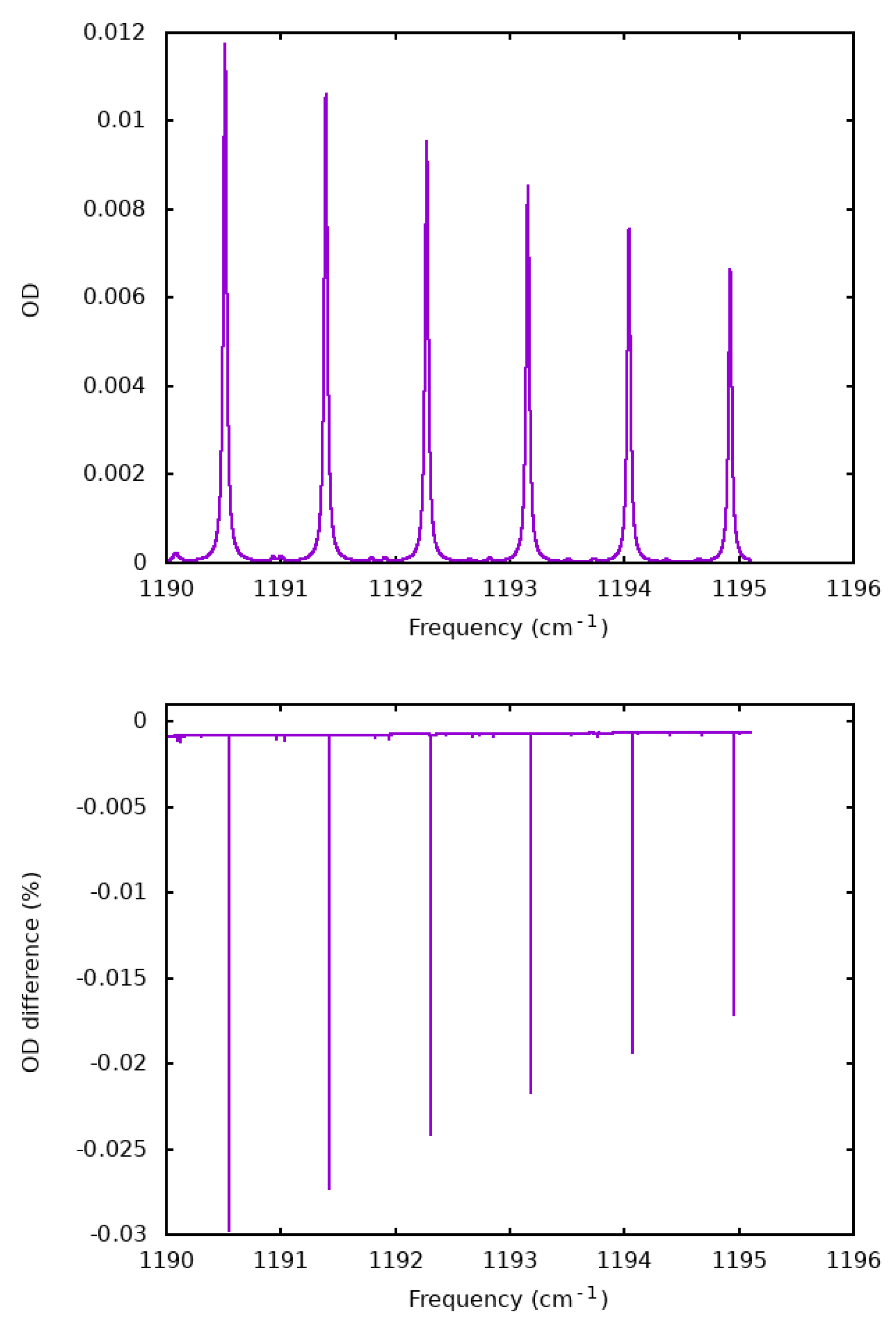
4.1. Comparison of the Optical Depths

The validation of the GBB-Nadir code started with a comparison of the optical depths (ODs) of single gases with the ones generated by KLIMA. In order to do this, GBB-Nadir and KLIMA were ran with the same spectroscopic database (AER 3.8), frequency step (2.5 $\times {10}^{-4}$ cm${}^{-1}$) and atmosphere. In particular the atmosphere was divided into 60 layers and for each layer the same values of pressure, temperature, air and gas columns used by KLIMA were used. As already explained in Section 2, GBB-Nadir computes the absorption cross-sections on a spectral grid that is tailored to the pressure and temperature of each layer and then linearly interpolated onto the final fine grid. This spectral grid may not coincide with the one used by the KLIMA code; therefore, we decided to inter-compare the ODs computing them directly onto the fine grid.

Therefore, both GBB-Nadir and KLIMA were forced to always use the fine grid (no interpolation performed). Figure 5 shows an example of the comparison of the ODs computed by GBB-Nadir and KLIMA for water vapour (all isotopes but $HDO$) in the GBB-Nadir MW number 73 (410–415.1 cm${}^{-1}$) for the bottom layer (pressure 1008.99 hPa and temperature 287.98 K, water vapour column 1.286 $\times {10}^{21}$ mol/cm${}^2$). The top panel of the figure shows the value of the ODs computed by GBB-Nadir, while the central and bottom panels show the differences between of ODs computed by GBB-Nadir and KLIMA using the percentage difference with respect to the maximum value the OD assumed in the GBB-Nadir MW. Correspondingly to the emission lines, as can be seen in the central panel of Figure 5, we found a relatively large difference in the form of the first derivative of the signal. The cause of this behaviour was that the frequency grid used by KLIMA to compute the ODs for each band ($ban{d}_0$: 0–650 cm${}^{-1}$, $ban{d}_1$: 640–1215 cm${}^{-1}$, $ban{d}_2$: 1205–2005 cm${}^{-1}$, $ban{d}_3$: 1995–2765 cm${}^{-1}$) was reconstructed starting from the initial frequency of the band and by recursively adding the frequency step. GBB-Nadir always divides the frequency region into intervals 5 cm${}^{-1}$ wide, and the frequency grid is reconstructed with the same strategy used by KLIMA, but the starting wave number is reset at the beginning of each interval. Thus, if the starting frequency of the MW is not a multiple of the high-resolution frequency step, there is a discrepancy between the KLIMA and GBB-Nadir frequency grids that increases with frequency in the interval of each KLIMA band. This source of error was eliminated making the GBB-Nadir code read and use the same frequency grid of the KLIMA. After this change (bottom panel of Figure 5), the differences between the optical depths of KLIMA and GBB-Nadir are of the order of 0.002%. In the intermediate layer ( layer 30, not shown here) the absolute value of the OD differences for water vapour is below $0.012\%$ and in the upper layer it is below $1.8·{10}^{-6}\%$. This difference is mainly due to the different approximation used by KLIMA and GBB-Nadir in representing the line shape. Despite both KLIMA and GBB-Nadir only using the Voigt function close to the line centre, and the Lorentz function elsewhere, the frequency at which the two line shapes are swapped is different. Furthermore, for $HDO$ the larger absolute value of the OD percentage difference with respect to the maximum is in the intermediate layer, and does not exceed $0.008\%$. The size of the differences suggest that they mainly depend on the numerical precision of the computations.

N${}_2$O has a large concentration in the intermediate layer (pressure 187.59 hPa, temperature 216.70 K, gas column = 3.95 $\times {10}^{16}$ mol/cm${}^2$), where its OD almost reaches $0.012$ in the analysed spectral region (1190–1195.1 cm${}^{-1}$) and the absolute OD difference are below $0.03\%$ of the maximum (see Figure 6). In the other atmospheric layers the differences range from 5 × 10${}^{-6}$% in the top layer to 0.02% in the bottom layer. These results confirm the findings for H${}_2$O and the dependency of the differences on the numerical precision of the used computer.

A separate check was performed for the CO${}_2$ ODs, since the GBB-Nadir code computes them in dedicated subroutines, one for the HITRAN approach to the LM (FLM) and one for the LBLRTM approach. The CO${}_2$ ODs computed by KLIMA with the LM approach of LBLRTM include the contribution of its continuum. Therefore, in computing the CO${}_2$ ODswith the LBLRTM approach GBB-Nadir included the same version of the CO${}_2$ continuum.

The results of the comparison of the CO${}_2$ ODs for the frequency interval 665–670.1 cm${}^{-1}$ are shown in Figure 7. This MW was selected because it shows a strong absorption of CO${}_2$, a large LM contribution and the largest discrepancy between the KLIMA and LBLRTM. We see in the central panel of Figure 7 that in the LBLRTM method the maximum percentage differences do not exceed $0.02\%$. This difference is further reduced in the HITRAN FLM approach, shown in the bottom panel of Figure 7.

In general the ODs computed by the GBB-Nadir code show very good agreement with those computed by the KLIMA code. However, it is worth pointing out the main causes of the discrepancies in the results. In almost all cases (except $HN{O}_3$ and the upper layers of $N_{2}O$ and CO${}_2$) the differences show peaks in single grid points, each of which are placed on the right side of an absorption line (see Figure 5 bottom panel). This may be due to a one-grid point shift of the point at which the switch between the Voigt and Lorentz line shapes occurs in the two codes. Moreover, in many cases, not shown here, the difference shows a step. This is caused by the fact that KLIMA calculates the contribution of all the absorption lines in the spectral range of $\pm 25$ cm${}^{-1}$ from their centre, whereas the GBB-Nadir excludes all the lines whose centre is further than 25 cm${}^{-1}$ from the borders of the considered MW, and only computes lines within the spectral range where the contribution to the cross-section is lower than the fixed threshold.

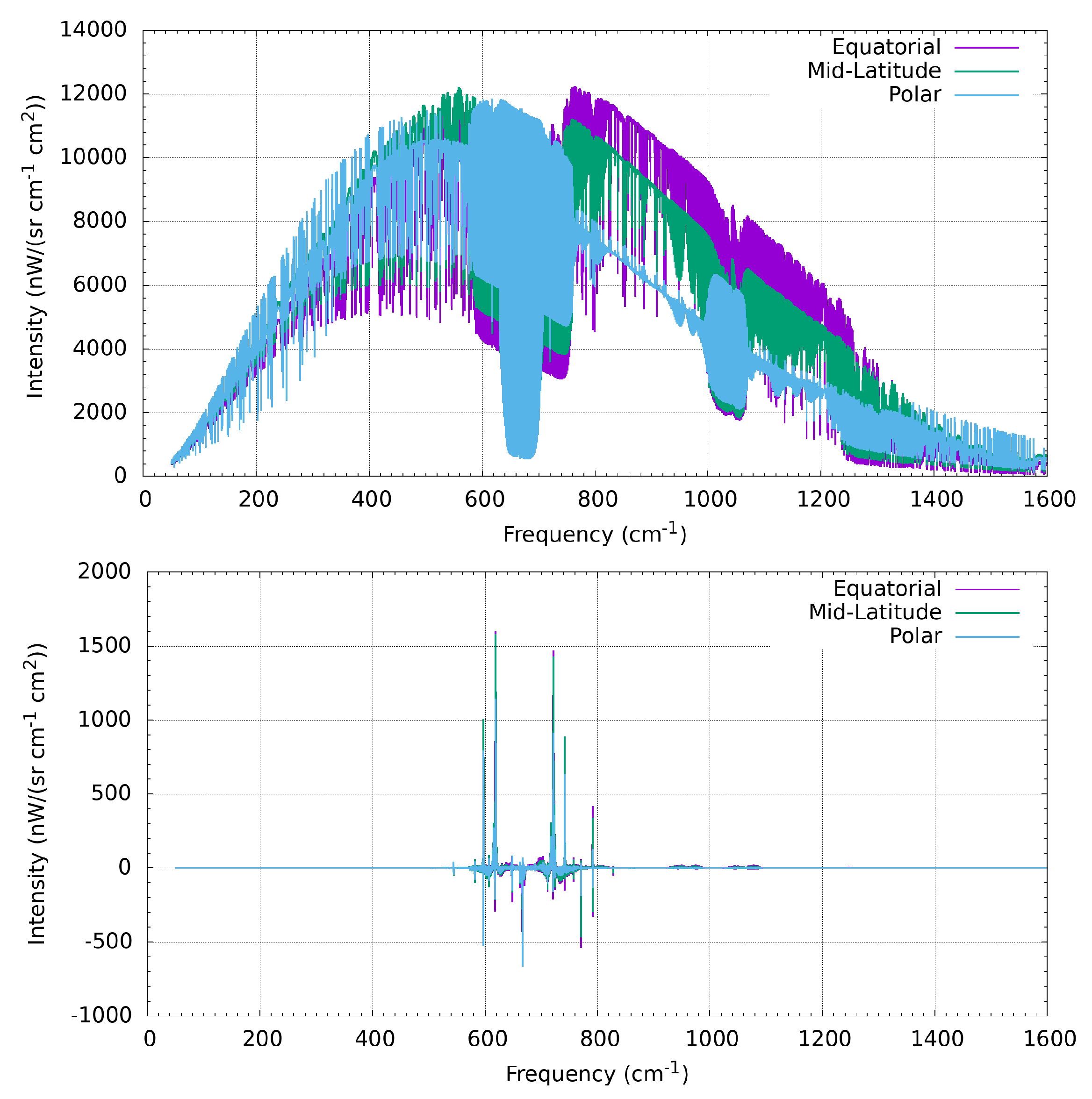
4.2. Validation of the Spectra

The radiances computed by GBB-Nadir were compared to the radiances computed by KLIMA, since, as described in Section 3 KLIMA was extensively compared to the widely used LBLRTM code [15]. The tests were performed using the same atmosphere in both codes. In order to highlight the possible problems due to the RTE solver, the same atmospheric stratification was used in both codes. Since the DISORT code implements an approximated form of the Plank function, while both the GBB-Nadir internal radiative transfer solver and KLIMA use the exact Plank expression, the radiances of the GBB-Nadir were computed with an internal solver. Separate tests were performed for two different spectroscopic databases: the AER v3.8 (using the LBLRTM CO${}_2$ line mixing implementation) and the HITRAN2020 spectroscopic databases (using the FLM model distributed by HITRAN). The spectra were compared at the FORUM instrument resolution, since we knew that the high-resolution grid used by KLIMA and GBB-Nadir were not completely coincident. As an example, in Figure 8 the differences between the spectra simulated with GBB-Nadir and KLIMA and convolved at the spectral resolution of FORUM are reported. They were compared to the expected FORUM noise level and to 1/10 of the FORUM noise. As shown in the two panels of Figure 8, the difference between the two simulations are mainly below the 1/10 FORUM noise level, with slightly better performances when the HITRAN2020 data were used. The differences are mainly due to the different threshold used when computing the Curtis–Godson integrals to compute the equivalent pressures and temperatures of the atmospheric layers.

5. Conclusions

In this paper, we have described two full physics codes, GBB-Nadir and KLIMA, both able to compute the spectrum of the Earth’s radiance escaping to space, while GBB-Nadir is only a forward model, computing the spectra only, KLIMA also implements the computation of the spectral radiance derivatives with respect to atmospheric parameters, and therefore suitable to be used in retrieval codes. KLIMA was extensively validated comparing its radiances to ones generated by the widely used LBLRTM code. Therefore, in this paper we used the KLIMA code to extensively validate the GBB-Nadir code in clear sky conditions. We have shown that the ODs computed by the two codes are in very good agreement, using both HITRAN2020 spectroscopic data and AER v3.8 data. The radiances, compared at the FORUM instrument resolution, show differences well below the expected noise of the FORUM instrument.

The GBB-Nadir code can also be interfaced with RTE solvers that include representation of multiple scattering, making the code suitable to compute the radiances in all-sky conditions. The limb version of the GBB-Nadir code has already been used to simulate the radiances measured at limb by the visible and infrared mapping spectrometer (VIMS) for Titan’s atmosphere [53,54] and by the Jovian infrared auroral mapper (JIRAM) for Jupiter’s ionosphere and atmosphere [55], while the KLIMA code was used to simulate the nadir and limb radiances for a Martian atmosphere with satisfactory results. Therefore, we may safely affirm that both codes can be used to simulate nadir measurements in planetary atmospheres.

References

1. Clough, S.A.; Iacono, M.J. Line-by-line calculation of atmospheric fluxes and cooling rates: 2. Application to carbon dioxide, ozone, methane, nitrous oxide and the halocarbons. J. Geophys. Res. Atmos. 1995, 100, 16519–16535. [Google Scholar] [CrossRef]
2. Turner, D.; Mlawer, E. The Radiative Heating in Underexplored Bands Campaigns. Bull. Am. Meteorol. Soc. 2010, 91, 911–923. [Google Scholar] [CrossRef]
3. Harries, J.; Carli, B.; Rizzi, R.; Serio, C.; Mlynczak, M.; Palchetti, L.; Maestri, T.; Brindley, H.; Masiello, G. The Far-infrared Earth. Rev. Geophys. 2008, 46. [Google Scholar] [CrossRef]
4. Loeb, N.G.; Mayer, M.; Kato, S.; Fasullo, J.T.; Zuo, H.; Senan, R.; Lyman, J.M.; Johnson, G.C.; Balmaseda, M. Evaluating CERES: Twenty-Year Trends in Earth’s Energy Flows From Observations and Reanalyses. J. Geophys. Res. Atmos. 2022, 127, e2022JD036686. [Google Scholar] [CrossRef]
5. Maestri, T.; Arosio, C.; Rizzi, R.; Palchetti, L.; Bianchini, G.; Del Guasta, M. Antarctic Ice Cloud Identification and Properties Using Downwelling Spectral Radiance from 100 to 1400 cm-1. J. Geophys. Res. Atmos. 2019, 124, 4761–4781. [Google Scholar] [CrossRef]
6. Cox, C.V.; Harries, J.E.; Taylor, J.P.; Green, P.D.; Baran, A.J.; Pickering, J.C.; Last, A.E.; Murray, J. Measurement and simulation of mid- and far-infrared spectra in the presence of cirrus. Q. J. R. Meteorol. Soc. 2010, 136, 718–739. [Google Scholar] [CrossRef]
7. Lubin, D.; Chen, B.; Bromwich, D.; Somerville, R.; Lee, W.H.; Hines, K. The Impact of Antarctic Cloud Radiative Properties on a GCM Climate Simulation. J. Clim. 1998, 11, 447–462. [Google Scholar] [CrossRef]
8. Baran, A.J. A review of the light scattering properties of cirrus. J. Quant. Spectrosc. Radiat. Transf. 2009, 110, 1239–1260. [Google Scholar] [CrossRef]
9. Huang, X.; Yang, W.; Loeb, N.G.; Ramaswamy, V. Spectrally resolved fluxes derived from collocated AIRS and CERES measurements and their application in model evaluation: Clear sky over the tropical oceans. J. Geophys. Res. Atmos. 2008, 113. [Google Scholar] [CrossRef]
10. Turner, E.C.; Lee, H.T.; Tett, S.F.B. Using IASI to simulate the total spectrum of outgoing long-wave radiances. Atmos. Chem. Phys. 2015, 15, 6561–6575. [Google Scholar] [CrossRef]
11. Formisano, V.; Angrilli, F.; Arnold, G.; Atreya, S.; Bianchini, G.; Biondi, D.; Blanco, A.; Blecka, M.; Coradini, A.; Colangeli, L.; et al. The Planetary Fourier Spectrometer (PFS) onboard the European Mars Express mission. Planet. Space Sci. 2005, 53, 963–974. [Google Scholar] [CrossRef]
12. Jennings, D.E.; Flasar, F.M.; Kunde, V.G.; Nixon, C.A.; Segura, M.E.; Romani, P.N.; Gorius, N.; Albright, S.; Brasunas, J.C.; Carlson, R.C.; et al. Composite infrared spectrometer (CIRS) on Cassini. Appl. Opt. 2017, 56, 5274–5294. [Google Scholar] [CrossRef] [PubMed]
13. Palchetti, L.; Brindley, H.; Bantges, R.; Buehler, S.A.; Camy-Peyret, C.; Carli, B.; Cortesi, U.; Bianco, S.D.; Natale, G.D.; Dinelli, B.M.; et al. FORUM: Unique Far-Infrared Satellite Observations to Better Understand How Earth Radiates Energy to Space. Bull. Am. Meteorol. Soc. 2020, 101, E2030–E2046. [Google Scholar] [CrossRef]
14. Dong, Y.; Proistosescu, C.; Armour, K.; Battisti, D. Attributing Historical and Future Evolution of Radiative Feedbacks to Regional Warming Patterns using a Green’s Function Approach: The Preeminence of the Western Pacific. J. Clim. 2019, 32, 5471–5491. [Google Scholar] [CrossRef]
15. Clough, S.; Shephard, M.; Mlawer, E.; Delamere, J.; Iacono, M.; Cady-Pereira, K.; Boukabara, S.; Brown, P. Atmospheric radiative transfer modeling: A summary of the AER codes. J. Quant. Spectrosc. Radiat. Transf. 2005, 91, 233–244. [Google Scholar] [CrossRef]
16. Coustenis, A.; Achterberg, R.K.; Conrath, B.J.; Jennings, D.E.; Marten, A.; Gautier, D.; Nixon, C.A.; Flasar, F.M.; Teanby, N.A.; Bézard, B.; et al. The composition of Titan’s stratosphere from Cassini/CIRS mid-infrared spectra. Icarus 2007, 189, 35–62. [Google Scholar] [CrossRef]
17. Bampasidis, G.; Coustenis, A.; Achterberg, R.K.; Vinatier, S.; Lavvas, P.; Nixon, C.A.; Jennings, D.E.; Teanby, N.A.; Flasar, F.M.; Carlson, R.C.; et al. Thermal and Chemical Structure Variations in Titan’s Stratosphere during the Cassini Mission. Astrophys. J. 2012, 760, 144. [Google Scholar] [CrossRef]
18. Liuzzi, G.; Masiello, G.; Serio, C.; Venafra, S.; Camy-Peyret, C. Physical inversion of the full IASI spectra: Assessment of atmospheric parameters retrievals, consistency of spectroscopy and forward modelling. J. Quant. Spectrosc. Radiat. Transf. 2016, 182, 128–157. [Google Scholar] [CrossRef]
19. Saunders, R.; Hocking, J.; Turner, E.; Rayer, P.; Rundle, D.; Brunel, P.; Vidot, J.; Roquet, P.; Matricardi, M.; Geer, A.; et al. An update on the RTTOV fast radiative transfer model (currently at version 12). Geosci. Model Dev. 2018, 11, 2717–2737. [Google Scholar] [CrossRef]
20. Ignatiev, N.; Grassi, D.; Zasova, L. Planetary Fourier spectrometer data analysis: Fast radiative transfer models. Planet. Space Sci. 2005, 53, 1035–1042. [Google Scholar] [CrossRef]
21. Casadio, S.; Castelli, E.; Papandrea, E.; Dinelli, B.; Pisacane, G.; Burini, A.; Bojkov, B. Total column water vapour from along track scanning radiometer series using thermal infrared dual view ocean cloud free measurements: The Advanced Infra-Red Water Vapour Estimator (AIRWAVE) algorithm. Remote Sens. Environ. 2016, 172, 1–14. [Google Scholar] [CrossRef]
22. Castelli, E.; Papandrea, E.; Roma, A.D.; Dinelli, B.; Casadio, S.; Bojkov, B. The Advanced Infra-Red WAter Vapour Estimator (AIRWAVE) version 2: Algorithm evolution, dataset description and performance improvements. Atmos. Meas. Tech. 2019, 12, 371–388. [Google Scholar] [CrossRef]
23. Del Bianco, S.; Carli, B.; Gai, M.; Laurenza, L.M.; Cortesi, U. XCO2 retrieved from IASI using KLIMA algorithm. Ann. Geophys. 2013, 56. [Google Scholar] [CrossRef]
24. Carlotti, M.; Dinelli, B.M.; Raspollini, P.; Ridolfi, M. Geo-fit approach to the analysis of limb-scanning satellite measurements. Appl. Opt. 2001, 40, 1872–1885. [Google Scholar] [CrossRef] [PubMed]
25. Ridolfi, M.; Carli, B.; Carlotti, M.; Clarmann, T.V.; Dinelli, B.M.; Dudhia, A.; Flaud, J.; Höpfner, M.; Morris, P.; Raspollini, P.; et al. Optimized forward model and retrieval scheme for MIPAS near-real-time data processing. Appl. Opt. 2000, 39, 1323–1340. [Google Scholar] [CrossRef]
26. Stamnes, K.; Tsay, S.; Wiscombe, W.; Jayaweera, K. Numerically stable algorithm for Discrete-Ordinate-Method radiative transfer in multiple scattering and emitting layered media. Appl. Opt. 1988, 27, 2502–2509. [Google Scholar] [CrossRef]
27. Spurr, R. LIDORT and VLIDORT: Linearized pseudo-spherical scalar and vector discrete ordinate radiative transfer models for use in remote sensing retrieval problems. In Light Scattering Reviews 3: Light Scattering and Reflection; Springer: Berlin/Heidelberg, Germany, 2008; pp. 229–275. [Google Scholar]
28. Rothman, L. History of the HITRAN Database. Nat. Rev. Phys. 2021, 3, 302–304. [Google Scholar] [CrossRef]
29. Mishchenko, M.I.; Travis, L.D.; Lacis, A.A. Scattering, Absorption, and Emission of Light by Small Particles; Cambridge University Press: Cambridge, UK, 2002. [Google Scholar]
30. Curtis, A. A statistical model for water-vapour absorption. Q. J. R. Meteorol. Soc. 1952, 78, 638–640. [Google Scholar] [CrossRef]
31. Godson, W. The evaluation of infra-red radiative fluxes due to atmospheric water vapour. Q. J. R. Meteorol. Soc. 1953, 79, 367–379. [Google Scholar] [CrossRef]
32. Gordon, I.; Rothman, L.; Hill, C.; Kochanov, R.; Tan, Y.; Bernath, P.; Birk, M.; Boudon, V.; Campargue, A.; Chance, K.; et al. The HITRAN2016 molecular spectroscopic database. J. Quant. Spectrosc. Radiat. Transf. 2017, 203, 3–69. [Google Scholar] [CrossRef]
33. Gamache, R.; Roller, C.; Lopes, E.; Gordon, I.; Rothman, L.; Polyansky, O.; Zobov, N.; Kyuberis, A.; Tennyson, J.; Yurchenko, S.; et al. Total internal partition sums for 166 isotopologues of 51 molecules important in planetary atmospheres: Application to HITRAN2016 and beyond. J. Quant. Spectrosc. Radiat. Transf. 2017, 203, 70–87. [Google Scholar] [CrossRef]
34. Humlícek, J. Optimized Computation of the Voigt and Complex Probability Functions. J. Quant. Spectrosc. Radiat. Transf. 1982, 27, 437–444. [Google Scholar] [CrossRef]
35. Lamouroux, J.; Regalia, L.; Thomas, X.; Auwera, J.V.; Gamache, R.; Hartmann, J.M. CO2 line-mixing database and software update and its tests in the 2.1 μm and 4.3 μm regions. J. Quant. Spectrosc. Radiat. Transf. 2015, 151, 88–96. [Google Scholar] [CrossRef]
36. Clough, S.A.; Iacono, M.J.; Moncet, J.L. Line-by-line calculations of atmospheric fluxes and cooling rates: Application to water vapor. J. Geophys. Res. Atmos. 1992, 97, 15761–15785. [Google Scholar] [CrossRef]
37. Carli, B.; Bazzini, G.; Castelli, E.; Cecchi-Pestellini, C.; Del Bianco, S.; Dinelli, B.; Gai, M.; Magnani, L.; Ridolfi, M.; Santurri, L. MARC: A code for the retrieval of atmospheric parameters from millimeter-wave limb measurements. J. Quant. Spectrosc. Radiat. Transf. 2007, 105, 476–491. [Google Scholar] [CrossRef]
38. Del Bianco, S.; Carli, B.; Cecchi-Pestellini, C.; Dinelli, B.M.; Gai, M.; Santurri, L. Retrieval of minor constituents in a cloudy atmosphere with remote-sensing millimetre-wave measurements. Q. J. R. Meteorol. Soc. 2007, 133, 163–170. [Google Scholar] [CrossRef]
39. Dinelli, B.M.; Castelli, E.; Carli, B.; Del Bianco, S.; Gai, M.; Santurri, L.; Moyna, B.P.; Oldfield, M.; Siddans, R.; Gerber, D.; et al. Technical Note: Measurement of the tropical UTLS composition in presence of clouds using millimetre-wave heterodyne spectroscopy. Atmos. Chem. Phys. 2009, 9, 1191–1207. [Google Scholar] [CrossRef]
40. Belotti, C.; Barbara, F.; Barucci, M.; Bianchini, G.; D’Amato, F.; Del Bianco, S.; Di Natale, G.; Gai, M.; Montori, A.; Pratesi, F.; et al. The Far-Infrared Radiation Mobile Observation System for spectral characterisation of the atmospheric emission. EGUsphere 2022, 2022, 1–34. [Google Scholar] [CrossRef]
41. Bianchini, G.; Carli, B.; Cortesi, U.; Del Bianco, S.; Gai, M.; Palchetti, L. Test of far-infrared atmospheric spectroscopy using wide-band balloon-borne measurements of the upwelling radiance. J. Quant. Spectrosc. Radiat. Transf. 2008, 109, 1030–1042. [Google Scholar] [CrossRef]
42. Ceccherini, S.; Cortesi, U.; Del Bianco, S.; Raspollini, P.; Carli, B. IASI-METOP and MIPAS-ENVISAT data fusion. Atmos. Chem. Phys. 2010, 10, 4689–4698. [Google Scholar] [CrossRef]
43. Tirelli, C.; Ceccherini, S.; Zoppetti, N.; Del Bianco, S.; Cortesi, U. Generalization of the complete data fusion to multi-target retrieval of atmospheric parameters and application to FORUM and IASI-NG simulated measurements. J. Quant. Spectrosc. Radiat. Transf. 2021, 276, 107925. [Google Scholar] [CrossRef]
44. Sgheri, L.; Belotti, C.; Ben-Yami, M.; Bianchini, G.; Carnicero Dominguez, B.; Cortesi, U.; Cossich, W.; Del Bianco, S.; Di Natale, G.; Guardabrazo, T.; et al. The FORUM end-to-end simulator project: Architecture and results. Atmos. Meas. Tech. 2022, 15, 573–604. [Google Scholar] [CrossRef]
45. Mazzoni, M.; Falorni, P.; Del Bianco, S. Sun-induced leaf fluorescence retrieval in the O2-B atmospheric absorption band. Opt. Express 2008, 16, 7014–7022. [Google Scholar] [CrossRef] [PubMed]
46. Caligiuri, C.; Barbara, F.; Barucci, M.; Belotti, C.; Bianchini, G.; Cortesi, U.; D’Amato, F.; Della Fera, S.; Del Bianco, S.; Dinelli, B.M.; et al. Poster: Feasibility Study of HDO Retrieval from FORUM-EE9 Measurements. In Proceedings of the Living Planet Symposium 2022, Bonn, Germany, 23–27 May 2022. [Google Scholar]
47. Laurenza, L.M.; Bianco, S.D.; Gai, M.; Barbara, F.; Schiavon, G.; Cortesi, U. Comparison of Column-Averaged Volume Mixing Ratios of Carbon Dioxide Retrieved From IASI/METOP-A Using KLIMA Algorithm and TANSO-FTS/GOSAT Level 2 Products. IEEE J. Sel. Top. Appl. Earth Obs. Remote Sens. 2014, 7, 389–398. [Google Scholar] [CrossRef]
48. Palchetti, L.; Bianchini, G.; Carli, B.; Cortesi, U.; Del Bianco, S. Measurement of the water vapour vertical profile and of the Earth’s outgoing far infrared flux. Atmos. Chem. Phys. 2008, 8, 2885–2894. [Google Scholar] [CrossRef]
49. Gordon, I.; Rothman, L.; Hargreaves, R.; Hashemi, R.; Karlovets, E.; Skinner, F.; Conway, E.; Hill, C.; Kochanov, R.; Tan, Y.; et al. The HITRAN2020 molecular spectroscopic database. J. Quant. Spectrosc. Radiat. Transf. 2022, 277, 107949. [Google Scholar] [CrossRef]
50. Lamouroux, J.; Tran, H.; Laraia, A.; Gamache, R.; Rothman, L.; Gordon, I.; Hartmann, J.M. Updated database plus software for line-mixing in CO2 infrared spectra and their test using laboratory spectra in the 1.5–2.3 μm region. J. Quant. Spectrosc. Radiat. Transf. 2010, 111, 2321–2331. [Google Scholar] [CrossRef]
51. Rodgers, C.D. Inverse Methods for Atmospheric Sounding; World Scientific: Singapore, 2000. [Google Scholar] [CrossRef]
52. Anderson, G.P.; Clough, S.A.; Kneizys, F.X.; Chetwynd, J.H.; Shettle, E.P. AFGL Atmospheric Constituent Profiles (0–120 km). 1986. Available online: https://apps.dtic.mil/sti/pdfs/ADA175173.pdf (accessed on 23 March 2023).
53. Adriani, A.; Dinelli, B.M.; López-Puertas, M.; García-Comas, M.; Moriconi, M.; D’Aversa, E.; Funke, B.; Coradini, A. Distribution of HCN in Titan’s upper atmosphere from Cassini/VIMS observations at 3 μm. ICARUS 2011, 214, 584–595. [Google Scholar] [CrossRef]
54. García-Comas, M.; López-Puertas, M.; Funke, B.; Dinelli, B.M.; Moriconi, M.L.; Adriani, A.; Molina, A.; Coradini, A. Analysis of Titan CH4 3.3 μm upper atmospheric emission as measured by Cassini/VIMS. ICARUS 2011, 214, 571–583. [Google Scholar] [CrossRef]
55. Dinelli, B.M.; Adriani, A.; Mura, A.; Altieri, F.; Migliorini, A.; Moriconi, M.L. JUNO/JIRAM’s view of Jupiter’s H3+ emissions. Philos. Trans. R. Soc. A 2019, 377, 20180406. [Google Scholar] [CrossRef]
Figure 1. Top panel: Spectral radiances simulated with GBB without accounting for CO 2 LM for equatorial (purple), mid-latitude (green) and polar (light-blue) atmospheres. Bottom panels: Difference between the spectrum simulated with the various methods to compute the LM for the CO 2 cross-sections and the same spectrum where the LM was not taken into account; top panel using FLM, central panel using the HITRAN SDV model, bottom panel using the LBLRTM SDV + continuum approach.
Remotesensing 15 02532 g001aRemotesensing 15 02532 g001b
Figure 2. Differences of the spectra (at FORUM resolution and over the FORUM spectral region) computed with the GBB-Nadir code using DISORT and the internal RT solver compared to the FORUM NESR divided by 10 (light blue lines), using the exact Plank function in the internal radiative transfer (purple line) or the DISORT approximated version of the Plank function (green line).
Remotesensing 15 02532 g002
Figure 3. Differences between KLIMA and LBLRTM radiance simulations for six standard scenarios (AFGL 1 to 6) compared with the nominal value of FORUM NESR in the FORUM band. (top) FORUM instrumental effects are not included. (bottom) FORUM instrumental effects are included.
Remotesensing 15 02532 g003aRemotesensing 15 02532 g003b
Figure 4. Differences between LBLRTM and monoRTM radiance simulations (green curve) and between KLIMA and monoRTM radiance simulations (red curve) compared with the nominal values of FORUM NESR (brown curve). Simulations refer to AFGL six standard scenario. Instrumental effects are not included.
Remotesensing 15 02532 g004
Figure 5. Top panel: H 2 O (all isotopes but H D O ) OD of the bottom layer (pressure 1008.99 hPa and temperature 287.98 K, water vapour column 1.286 × 10 21 mol/cm 2 ) computed by GBB-Nadir in the spectral region 410–415.1 cm 1 . Central panel: percentage difference of the H 2 O OD computed by GBB-Nadir and KLIMA in the two native frequency grids. Bottom panel: percentage difference of the H 2 O OD computed by GBB-Nadir and KLIMA using the same frequency grid.
Remotesensing 15 02532 g005aRemotesensing 15 02532 g005b
Figure 6. Top panel: N 2 O (all isotopes) OD of the intermediate layer computed by GBB-Nadir in the spectral region 1190–1195.1 cm 1 . Bottom panel: percentage difference (relative to the maximum value of the OD in the MW) of the N 2 O OD computed by GBB-Nadir and KLIMA using the same frequency grid.
Remotesensing 15 02532 g006
Figure 7. Top panel: CO 2 ODs computed by GBB-Nadir for the bottom layer. Central and bottom panels: percent difference between the ODs computed by GBB-Nadir and KLIMA with respect to the maximum OD in the micro-window for the layer using the LBLRTM method and AER v3.8 data (centre) and FLM method and HITRAN2020 data (bottom).
Remotesensing 15 02532 g007
Figure 8. Top panel: differences between the simulated spectra of GBB-Nadir and KLIMA using the AER V3.8 database and the LBLRTM line mixing model for equatorial (purple), mid-latitude (green) and polar (light blue) atmospheres. Bottom panel: the same differences but using HITRAN2020 and the full line mixing model. The differences (purple line) are compared to the FORUM noise (yellow lines) and the FORUM noise divided by 10 (blue lines).
Remotesensing 15 02532 g008aRemotesensing 15 02532 g008b