Volume Loss Assessment with MT-InSAR during Tunnel Construction in the City of Naples (Italy)

Abstract

The construction of tunnels in urban areas can affect the nearby existing infrastructures and buildings, as shallow excavations induce movements up to the ground surface. An important parameter to be monitored during the excavation is the volume loss, which plays a crucial role in determining the ground movements at the surface. InSAR satellite monitoring has the potential to detect ground movements at the millimetric scale on a vast area for tunneling applications. In the present study, the Multi-Temporal InSAR (MT-InSAR) technique, based on the persistent scattering method, is used to retrieve vertical displacements induced by the excavation of twin tunnels of a metro line in the City of Naples (Italy). Here, the volume loss is obtained by fitting a Gaussian curve on the monitored settlement data induced by the excavation of the first tunnel. The latter is then used to predict the settlement of the second excavation about one year later and compared to the MT-InSAR data. These monitored data show the typical shape of the settlement profile, confirming the empirical Gaussian distribution and MT-InSAR capability to detect millimetric displacements. Therefore, MT-InSAR can be used to feed algorithms to improve the prediction of tunneling-induced displacements.

1. Introduction

The need for new infrastructures in densely populated cities due to the increasing global population [1], as well as the increasing migration from rural to urban areas [2], must be satisfied. Intensive land use in the previous decades has saturated the space for the creation of new superficial infrastructures (i.e., roads, railways, and so on). Thus, the demand for mobility is directed towards the exploration of the still intact underground space, where it can be satisfied through the construction of underground infrastructures, including tunnels.

Tunnel excavation in developed areas, while a delicate task to accomplish, may also pose a risk to the surrounding space, because the potential of causing damage to the nearby infrastructures and environment during the construction process. In fact, as urban tunnels are generally shallow, the field of displacements induced in the ground by the excavation propagates up to the ground level. This can be limited by implementing the appropriate engineering solutions, but not completely avoided. The prediction and monitoring of ground movements is thus a critical issue to assess potential damage and to undertake preventative measures [3,4].

The excavation of a tunnel in urban areas can affect buildings in multiple ways, depending on the excavation technique, depth and length of excavation, ground conditions, as well as many other factors. Considering the relatively high number of buildings potentially affected by the excavation in urban areas, it is often impossible to monitor them all with traditional monitoring techniques, owing to the prohibitive cost. Therefore, often only those buildings or infrastructures that have cultural, historical, and public relevance are monitored, or those that have been a priori identified as vulnerable according to the results of empirical or numerical methods.

In the last decades, processing of data from synthetic aperture radar (SAR) satellites was used to obtain information on deformation processes of the Earth’s surface, caused by various phenomena including, but not limited to, earthquakes [5,6,7], natural subsidence [8,9], and volcanic movements [10,11].

The recent development of high-resolution SAR satellites, such as the COSMO-SkyMed (CSK) (Constellation of Small Satellites for Mediterranean basin Observation) constellation or TerraSAR-X constellation, along with recent advancement in data processing techniques, such as the multi-temporal interferometric synthetic aperture radar (MT-InSAR), showed the capability to measure the field of displacements induced by tunnel excavations in urban areas [12,13,14,15].

In [12], the authors used a single Master persistent scatters (PS) analysis carried out on CSK descending SAR images for the detection of surface settlements induced by Shanghai subway tunnels, in China. The velocity map of deformations clearly indicated the subway alignment. InSAR-monitored velocities were fitted with a standard Gaussian distribution along tunnel cross sections, and a comparison with published data in the same area confirmed the extension of the fitted settlement trough. A similar work was carried out by [16]. Here, MT-InSAR is applied to the excavation of Metro Line 6 in the city of Naples, using CSK SAR images in ascending direction. The authors projected InSAR-monitored data in the vertical direction first, and then compared their time series to the traditional surveying method (precise levelling points, PLP), showing a good agreement. Furthermore, in order to analyze the spatial distribution of the settlements, the researchers applied a standard Gaussian curve to fit the InSAR and PLP data. This analysis revealed a strong correlation between the two monitoring techniques, despite the fact that only a small number of scatterers was taken into account.

A different approach was used in [13]. Here, the authors carried out an MT-InSAR analysis on CSK SAR images in both the ascending and descending direction. This allowed the separation of vertical and east–west (E–W) horizontal displacement components, induced by the excavation of two motorways tunnels. The InSAR results agree well with the conventional survey (robotic total station and automatic GPS), confirming the trend and the magnitude of displacements, in both the vertical and E–W horizontal directions.

A collection of interesting works pertaining to the post-tunneling building damage assessment procedure with InSAR data is provided in [14,15,17,18]. These latter papers focused on the Crossrail twin tunnels project in London, UK. A single Master MT-InSAR analysis was carried out on CSK descending SAR images. Standard Gaussian distribution or modified Gaussian distribution was used to fit the transverse profile of monitored settlements, in order to take into account the soil–structure interaction. From the traditional survey, an average value of volume loss V_L = 0.7%, with a standard deviation of 0.3%, was observed. The average inflection point distance from the tunnel axis was 0.5·z₀, with a standard deviation of 0.1·z₀ (with z₀ being the tunnel axis depth). InSAR data fitting with modified Gaussian reported values of volume loss in the range 0.7–1.4% for 12 out of 14 transverse sections considered by the authors, with an average value of 1.1%. The fitted inflection point was located within 1.9·z₀ for 12 out of 14 transverse sections, with an average value of 0.75·z₀. In [14], an example of a comparison between the InSAR settlement profile and the traditional survey (PLP) is provided, showing a good agreement. In general, the authors showed how InSAR can be used to detect settlements caused by tunneling, which enabled them to assess the extent of damage to over 800 buildings in London.

However, two main limits were identified for the use of MT-InSAR as a tool to perform real-time monitoring [19]: the satellite revisit time and the phase ambiguity. The first limit does not allow real-time monitoring to be performed on processes that are bounded in a small temporal baseline. The second limit influences the ability of MT-InSAR to detect displacements higher than λ/4, if the motion can change direction, or λ/2, if the motion is monotonic, between two consecutive acquisitions and two adjacent pixels [20] (where λ is the sensor’s wavelength).

Nevertheless, the presence of an image database allows for a posteriori analyses to support the development of advanced damage assessment procedures. Therefore, the objective of this study is to show an application and validation of this satellite monitoring technique related to the excavation of twin tunnels for the metro line in the city of Naples (Italy).

As far as the study area is concerned, 237 X-band images from the COSMO-SkyMed constellation in ascending geometry were selected for interferometric processing, covering the observation period from 7 March 2018 to 29 January 2022. This timeframe corresponds to the excavation of both twin tunnels. Images were analyzed with the software SARPROZ [21], using the MT-InSAR technique. The results of the analysis carried out during the excavation of the first tunnel were used to obtain tunnel-transverse settlement profiles. These were then used to calibrate established empirical methods [22,23] and improve the prediction of subsequent excavation of the second tunnel.

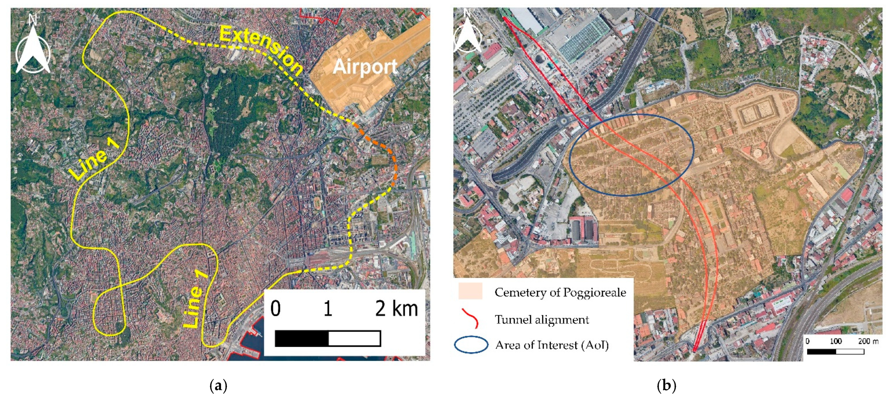
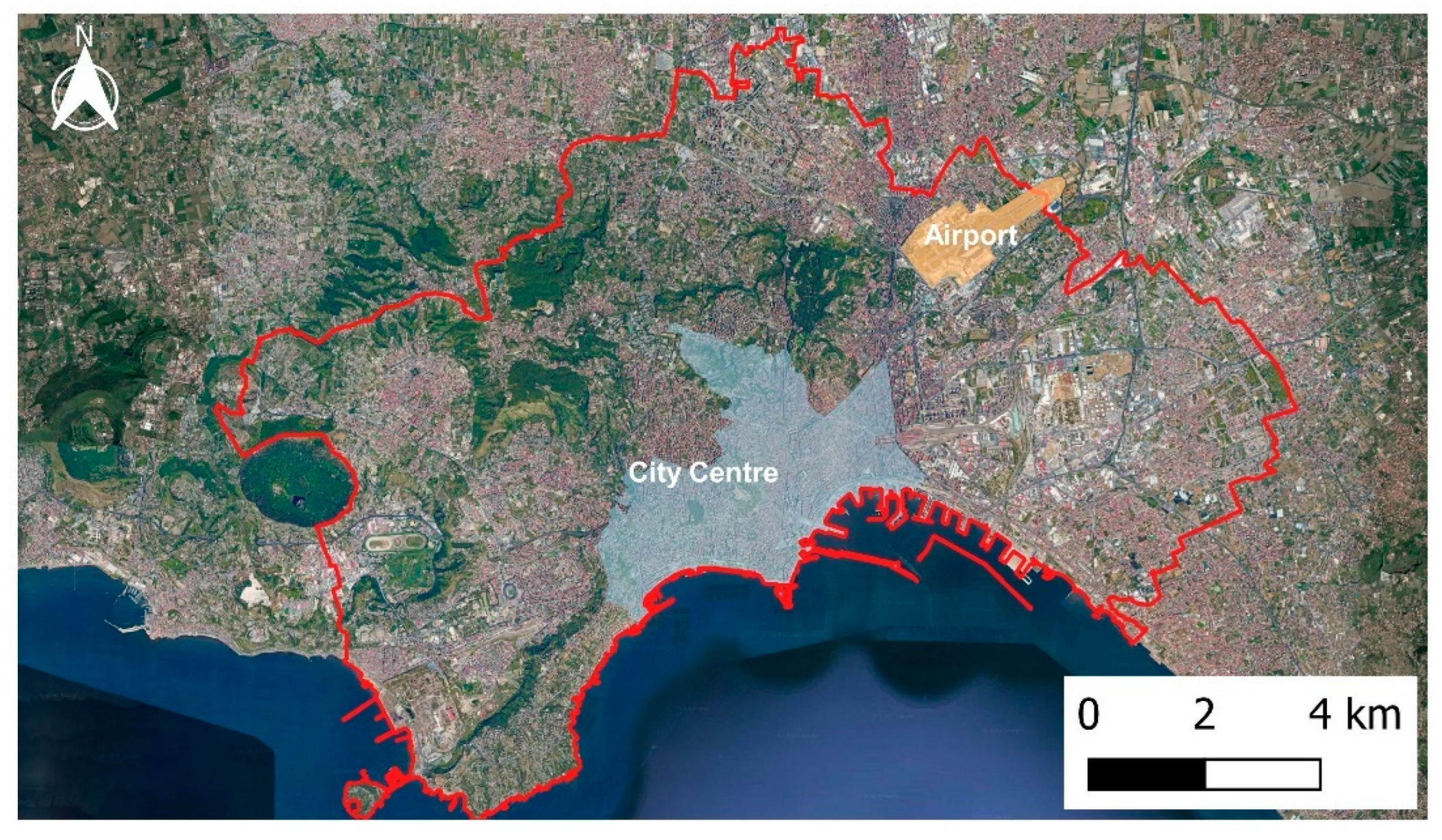
2. Area of Interest and Dataset

The city of Naples lies on the west coast of the Italian peninsula, about 200 km south-east of Rome. With a population of almost a million, it is the third largest city in Italy after Rome and Milan. Its prominent position on the coast of the Mediterranean Sea, flanked by natural and historical beauties and a warm climate, make it one of the most attractive destinations for tourists during the summer season, with peaks reaching 3.7 million tourists [24]. Many arriving by air transportation must connect through the only airport in the city, known as Capodichino Airport. The latter is located in the north-east area of the city (Figure 1), about 4 km away from the city center, and currently it is connected only by road transport to the urban center (unless specifically stated, all subsequent figures are oriented such that the vertical upward direction indicates north and, consequently, the horizontal rightward direction indicates east).

Commuters are limited to road transport and are subjected to daily heavy traffic. Therefore, to increase mobility between the airport and the city center, the City Council of Naples decided to contract out the extension of the existing Line 1 (Figure 2a) of the metro system, thus connecting the main train station to Capodichino Airport.

Two tunnels, one for each direction, were designed along the stretch between the two upcoming metro stations of Capodichino and Poggioreale (Figure 2b). The excavation of the first tunnel started from the shaft at Capodichino in July 2020 [25] and ended on 30 March 2021 [26]. The length of the excavation is roughly 1000 m per tunnel and it was performed using a tunnel boring machine (TBM) with a cutterhead of 7 m in diameter, mainly in a soft rock layer (‘ignimbrite campana’) covered by sandy and silty sand deposits [27]. The excavation of the first tunnel started 40 m below ground level from the shaft made for Capodichino station and arrived at Poggioreale station at 10 m below ground level [25,26]. The TBM was then disassembled and moved back to the Capodichino shaft, and used for the excavation of the second tunnel.

Figure 2. (a) Metro Line 1 of the city of Naples. The existing line is represented with a continuous line, while the extension is represented with a dashed line. In dashed orange, the segment Capodichino-Poggioreale. (b) Google Earth map of the area of interest (in blue). Red lines represent the longitudinal axes of the excavated tunnels (after [27]). In orange, the cemetery of Poggioreale (image modified after Google Earth, Google).

Figure 2. (a) Metro Line 1 of the city of Naples. The existing line is represented with a continuous line, while the extension is represented with a dashed line. In dashed orange, the segment Capodichino-Poggioreale. (b) Google Earth map of the area of interest (in blue). Red lines represent the longitudinal axes of the excavated tunnels (after [27]). In orange, the cemetery of Poggioreale (image modified after Google Earth, Google).

In this study, synthetic aperture radar (SAR) images were obtained from the Italian Space Agency (ASI) dataset. SAR images were acquired by the first generation of the COSMO-SkyMed satellites. The constellation consists of four low Earth orbit (≈600 km) satellites, each of them carrying an X-band SAR antenna with a repeat cycle of 16 days over the major cities of the world. The images can be acquired primarily in three modes: Spotlight mode, which acquires single polarized SAR images at a very high spatial resolution (1 m or lower), covering an area up to 100 km² (10 × 10 km); Stripmap mode, which acquires single or double polarized SAR images at a medium-high spatial resolution (3–15 m), covering an area up to 1600 km² (40 × 40 km); and ScanSAR mode, which acquires single polarized SAR images at a low spatial resolution (30–100 m), covering an area up to 40,000 km² (200 × 200 km).

Our dataset is formed by a stack of 237 CSK Stripmap-Himage collected in an ascending path direction from 7 March 2018 to 29 January 2022, and covers an area of 40 × 40 km at 3 m resolution in both the azimuth and range directions (i.e., along track and cross track directions, respectively). The reflectivity map (RM), i.e., the average amplitude of the microwave signal in the area, is shown in Figure 3a, while in Figure 3b, a subset of RM representing the analyzed area is shown. The timeline of image acquisition is presented in Figure 4, where the more frequent acquisition period is 16 days.

3. Methodology

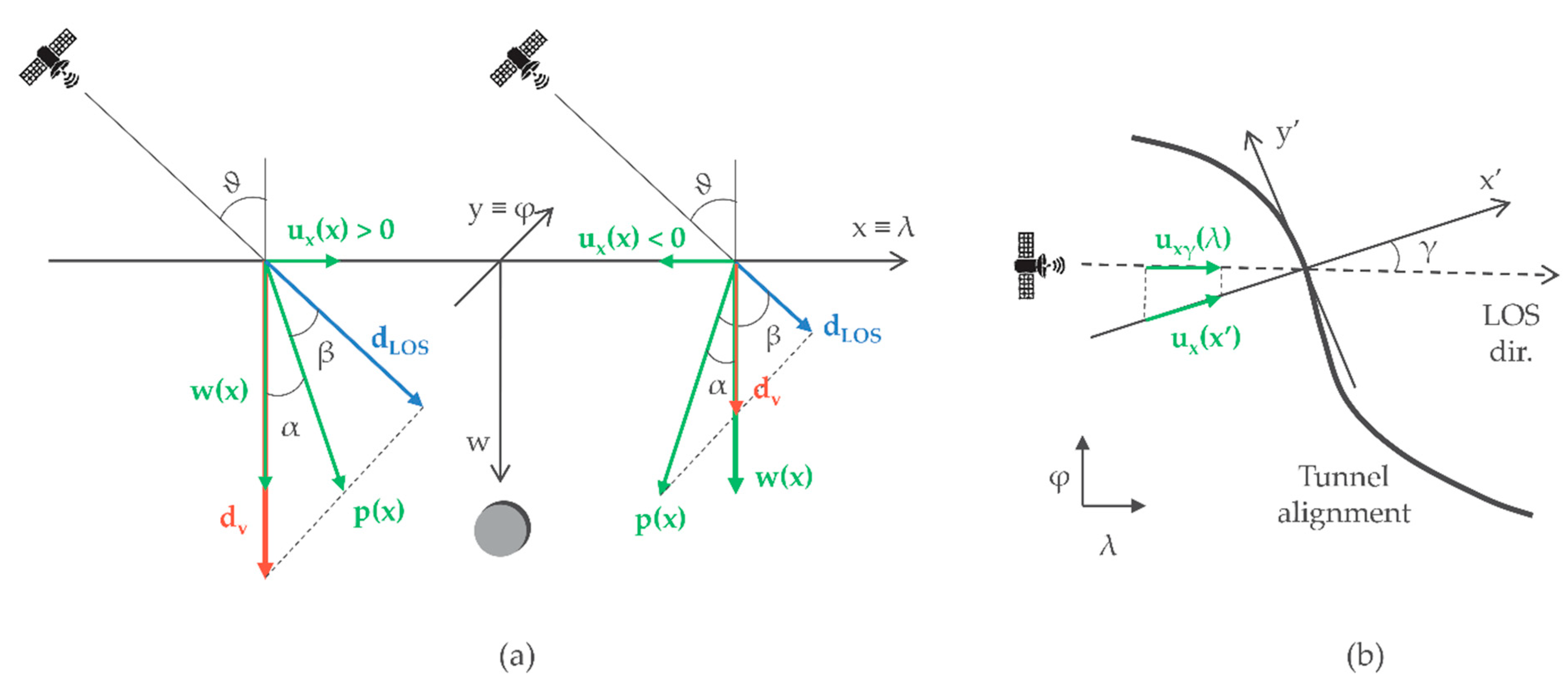
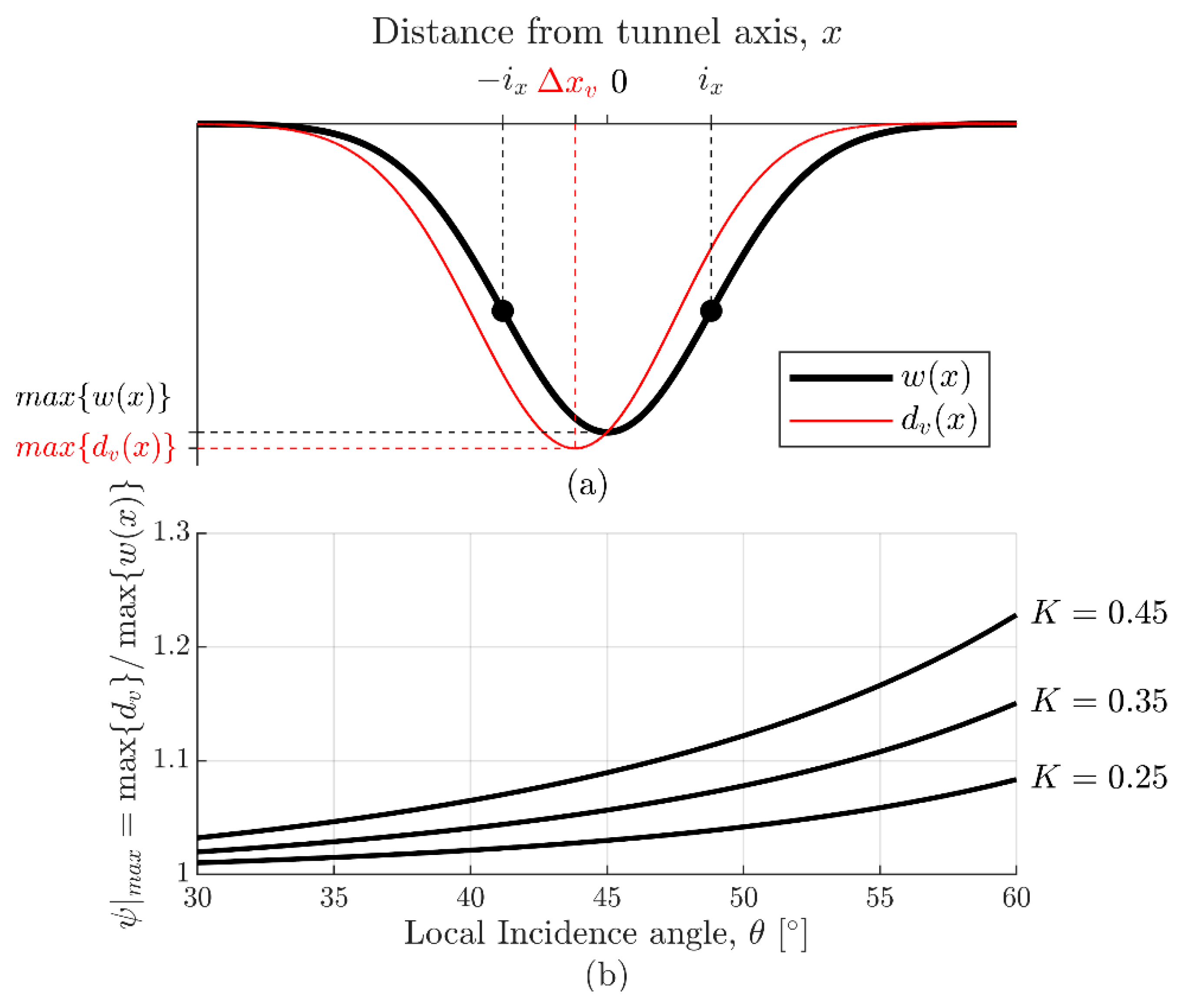
3.1. Empirical Method for Tunnel-Induced Vertical Displacements

The excavation of tunnels in greenfield conditions, or free-field (i.e., without buildings), induces a settlement trough at the surface. Far from the excavation face, plane strain conditions are assumed, and the transverse section of the greenfield settlement trough is well described by a Gaussian curve [22,23] as follows:

w(x) = w_max∙exp[−x²/(2∙i_x²)],

(1)

where w_max is the maximum settlement and i_x is the distance of the inflection point location from x = 0, as displayed in Figure 5a for clarification.

Integrating Equation (1), the volume of the settlement trough is equal to the following:

V_C = √(2π)∙i_x∙w_max.

(2)

In general, it can be assumed that V_C is a fraction of the excavated volume per unit length of advancement and this fraction is called ‘volume loss’, V_L. Therefore, the maximum settlement can be expressed as follows:

w_max = V_L∙√(2π)∙D²/(8∙i_x) = 0.31∙V_L∙D²/i_x.

(3)

Thus, it is evident that a correct prediction of the settlement trough depends on a reliable estimate of the parameter V_L and i_x. In the case of mechanized excavation with a tunnel boring machine (TBM), in general, the volume loss V_L rarely exceeds 1–1.5%, with usual values of 0.5%. For the inflection point distance i_x, it can be seen as a fraction K of the tunnel axis depth z₀ (i_x = K·z₀), with K ranging from 0.25 to 0.45 for sands and gravels and from 0.4 to 0.6 for clay [28,29].

Therefore, substituting Equation (3) in Equation (1) leads to the following:

w(x) = 0.31∙V_L∙D²/i_x∙exp[−x²/(2∙i_x²)].

(4)

In the case of twin tunnels, the superposition of the effects is often used to obtain the total ground surface settlement profile, as results of its speed and simplicity (Figure 5b,c). The superposition method involves a direct combination of two settlement troughs induced by each single tunnel excavated in greenfield conditions, without considering any interference between the two excavations. This can result in a misestimation of the total settlement profile [30,31]. When superimposing the effects of the twin tunnels, it is important to consider the distance Δx between them and the interaction between the two tunnels [32,33]. The distance Δx between two tunnels determines the shape of the total settlement profile. Generally, when Δx < 2·i_x, the total settlement profile still preserves a Gaussian shape, as shown in Figure 5b.

Conversely, when Δx > 2·i_x, the total settlement profile exhibits two peaks corresponding to the tunnel axes, as shown in Figure 5c.

To obtain the total settlement profile, a single value for both the volume loss V_L and the inflection point position i_x can be used, provided that the excavation process is identical and the ground conditions are the same for both tunnels:

w_tot(x) = 0.31∙V_L∙D²/i_x∙{exp[−x²/(2∙i_x²)] + exp[−(x + Δx)²/(2∙i_x²)]}.

(5)

Equation (5) gives a reliable estimate for the total settlement profile when tunnels are aligned side by side and their axes distance is greater than 2·D, such that the excavation process of the second tunnel does not influence the first.

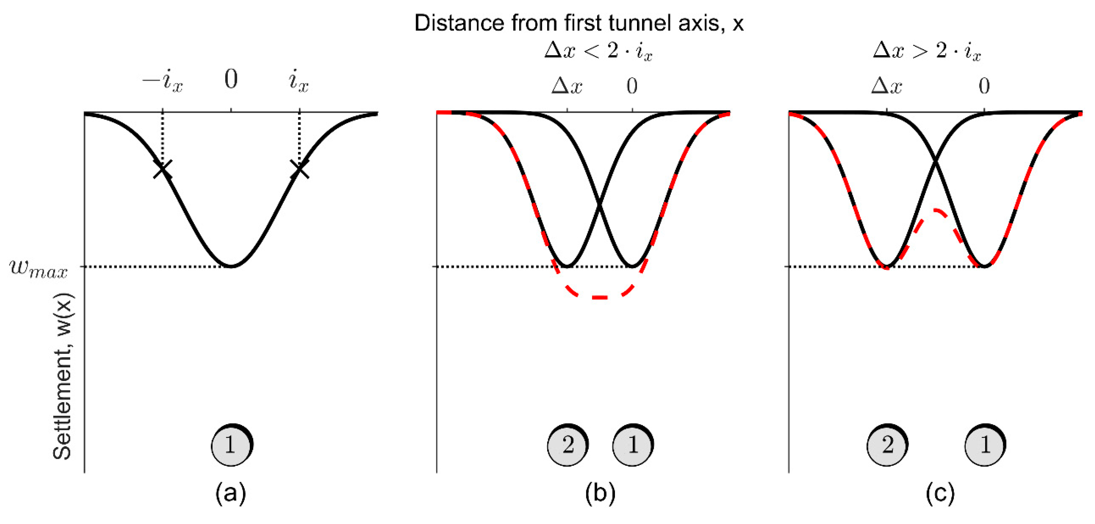
3.2. Empirical Method for Tunnel-Induced Horizontal Displacements

During the excavation of tunnels, horizontal displacements arise simultaneously with vertical displacements, with lateral movements directed toward the center of the trough. In greenfield conditions, past experience with the observational method [34,35], justified the theoretical assumption that considers displacement vectors directed toward the tunnel axis, thus relating the horizontal surface movements u_x to vertical ones w [28,36], as follows:

u_x(x) = w(x)∙x/z₀.

(6)

From the latter, the maximum horizontal displacement is attained for x = i_x, and substituting Equation (4) into Equation (6), one obtains the following:

u_x,max = 0.61∙K∙w_max,

(7)

which, for typical values of K in sandy soils or clays, leads to a maximum horizontal displacement in the range of (0.15 ÷ 0.28)∙w_max and (0.25 ÷ 0.40)∙w_max, respectively.

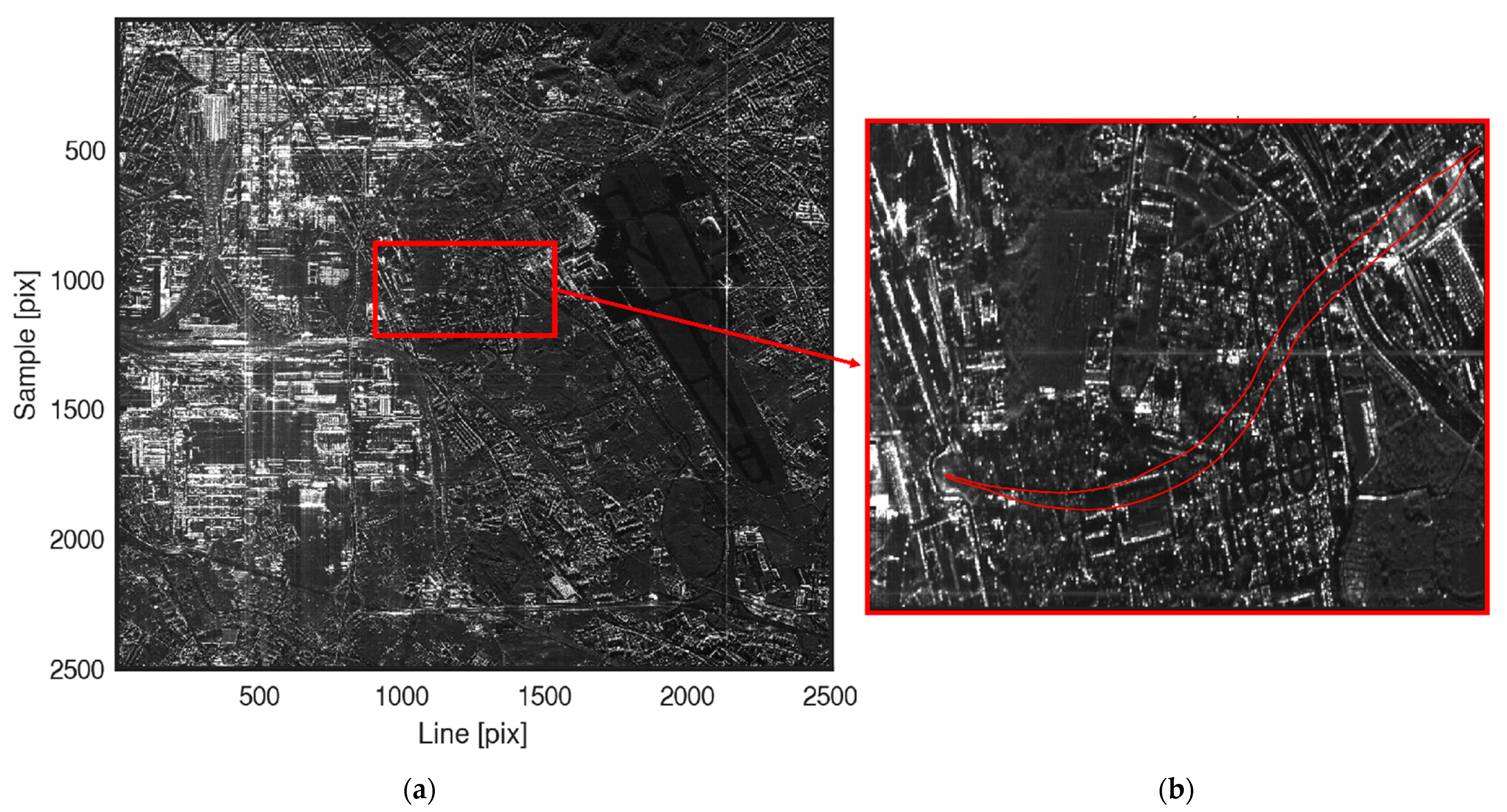
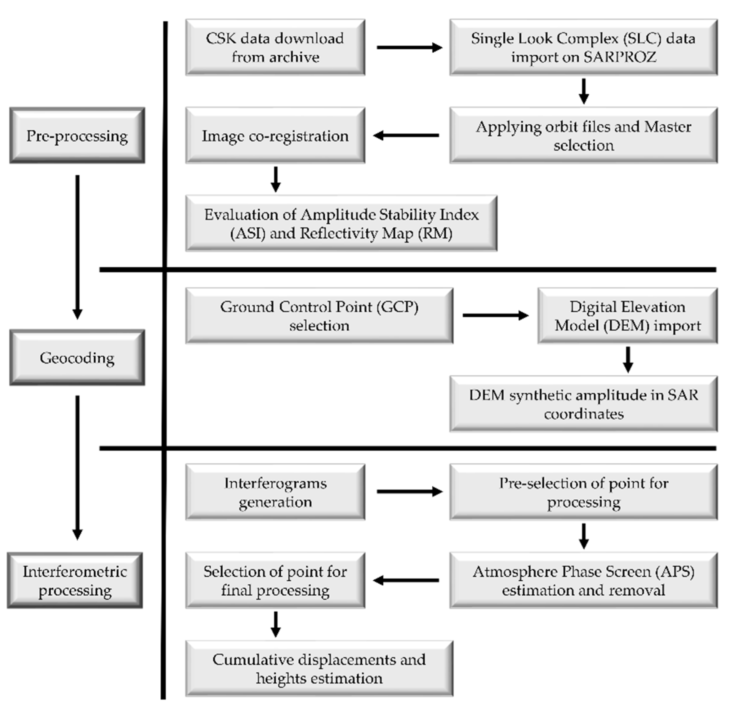
3.3. Multi Temporal InSAR

Interferometric synthetic aperture radar (InSAR) is a well-established technique suitable for detecting ground movements. It is based on the measurement of the phase shift ∆φ between two radar signals, which is a fraction of the wavelength λ. As InSAR satellites emit signals in the microwave region of the electromagnetic spectrum (λ = 3.1 cm for CSK satellites), it is possible to detect movements with the millimetric precision during the day and night and variable meteorological conditions. The limit of this application is due to spatial–temporal signal decorrelation, particularly in areas where there is a progressive change in the scattering properties of the targets, such as forests, harvesting fields, and so on. Indeed, interferometric coherence γ is a measure of the correlation between two radar signal and ranges from 0 to 1 (i.e., from total decorrelation to total correlation). Atmosphere artifacts are another limiting phenomena that delay radar signal, reducing the coherence of the pixels in the radar images. To overcome this limit, methods such as permanent scatter interferometry (PSI) [37] or small baseline subset (SBAS) [38] were developed in the early 2000s. For further technical insights, the reader is invited to refer to the following works: [21,37,39,40].

This work uses the PSI method, consisting of detecting pixels that show high coherence to retrieve the displacement map (better known as velocity map, mm/year) of the area of interest, using the software SARPROZ [21]. A flowchart of the data processing is presented in Figure 6.

A single Master PS linear analysis was adopted in this framework. PSs were selected using a coherence threshold of 0.5, which led to roughly 20,000 scatterers in the AoI, with a point density of 30,000 scatterers/km².

For each scatterer, temporal series were interpolated using four linear regressions (see Figure 7), one per each following period.

-

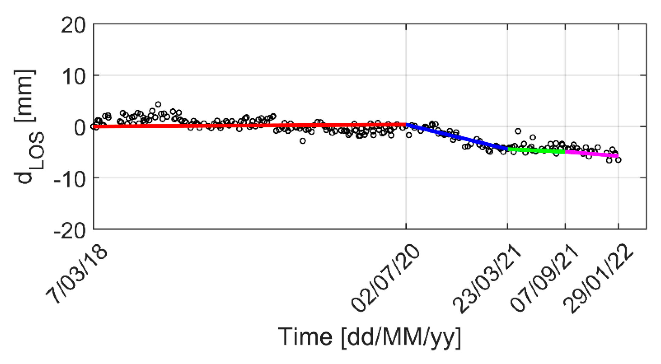
7 March 2018 to 2 July 2020 (i.e., from beginning of the analysis to prior to the first excavation);

-

2 July 2020 to 23 March 2021 (i.e., from the beginning to the end of the first excavation);

-

23 March 2021 to 7 September 2021 (i.e., from the end of the first excavation to the beginning of the second excavation);

-

7 September 2021 to 29 January 2022 (i.e., from the beginning of the second excavation to the end of the analysis).

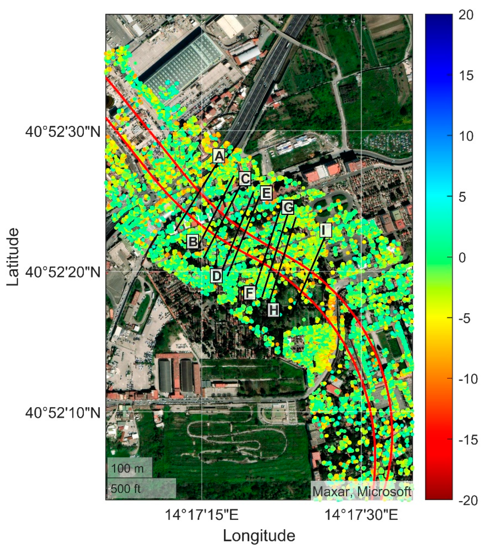
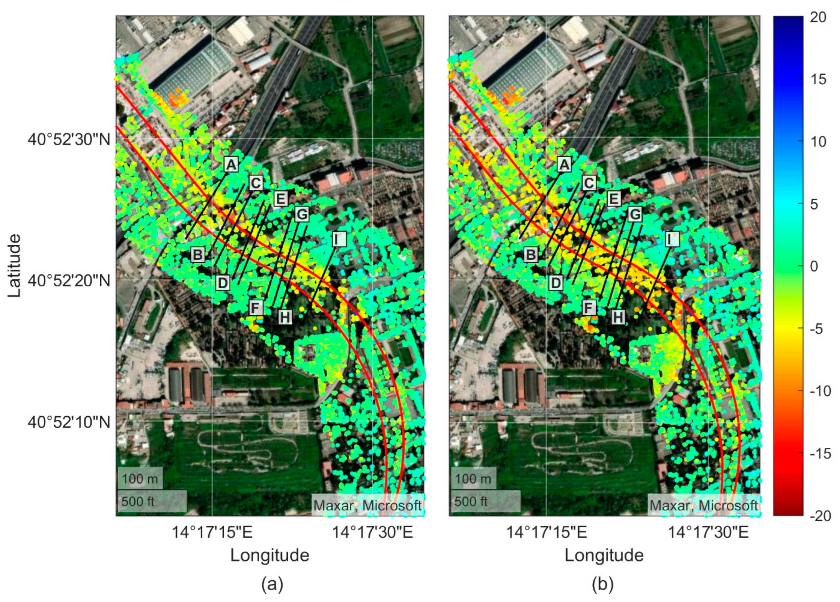
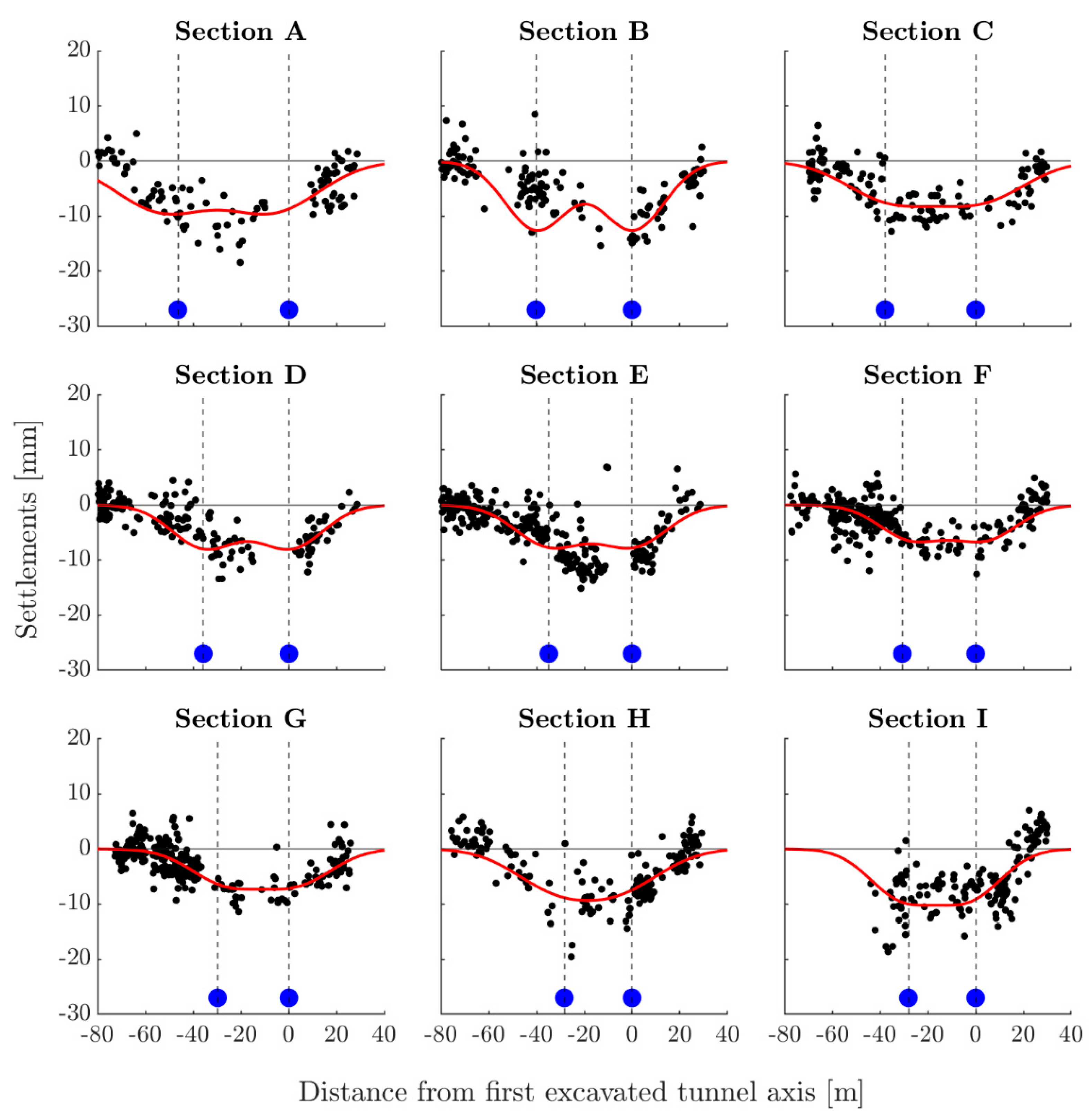
From those interpolations, line of sight (LOS) cumulative displacements were obtained on 2 July 2020, 23 March 2021, and 29 January 2022.

By considering a reference point very close to the study area, the local topography, and the expected deformational processes, it is common to assume that the movements that occurred in these periods, owing to tunneling, are predominantly vertical [15,18].

For this reason, LOS displacements can be converted into vertical displacements (settlements) according to Equation (8):

d_v = d_LOS/cos(ϑ),

(8)

where d_LOS is the displacement in the direction of the satellite line of sight (LOS) and ϑ is the local incidence angle of the satellite LOS direction to the vertical.

Nevertheless, it is crucial to assess the implications of this assumption. Considering the geometrical scheme of Figure 8a, i.e., when the tunnel cross section is contained in the LOS plane and the satellite is acquiring in ascending geometry, the intensity p(x) and the direction α(x) (to the vertical, positive if anticlockwise) of the actual (theoretical) displacement vector p(x) can be computed with the following:

|p(x)| = p(x) = (w(x)² + u_x(x)²)^0.5,

(9)

α(x) = atan(x/z0).

(10)

Then, the intensity of the monitored displacements along the LOS can be computed as follows:

d_LOS (x) = p(x)·cos(β(x)) = p(x)·cos(ϑ − α(x)),

(11)

with β(x) being the angle formed by the vectors p(x) and d_LOS(x). Finally, substituting Equation (11) into Equation (8), the projected displacement in the vertical direction is obtained as a function of the actual displacement intensity p(x):

d_v(x) = p(x)·cos(ϑ − α(x))/cos(ϑ),

(12)

And, by taking the ratio with w(x), it is possible to assess the error ψ(x) implied in the assumption of pure vertical displacements:

ψ(x) = d_v(x)/w(x) = cos(ϑ − α(x))/[cos(ϑ)·cos(α(x))] = 1 + x·tan(ϑ)/z₀.

(13)

From Figure 8a, it can be seen that, for negative values of x (i.e., left side of tunnel axis), the error is ψ(x < 0) > 1, while for positive values of x, the error is 0 < ψ(x < 0) < 1. Figure 9a shows the comparison between w(x) and d_v(x). It can be noted that, in the case of tunneling monitoring, when one converts the LOS displacements in vertical direction, the shape of the settlement profile is preserved (i.e., Gaussian distribution), but there is an overall increase in magnitude and a shift toward the satellite of the settlement profile.

The quantification of the maximum settlement’s increment is explicated through the expression ψ|_max = max{d_v(x)}/max{w(x)}, the determination of which depends exclusively on the local angle of incidence ϑ and the geotechnical parameter K, as shown in Figure 9b. The shift of the settlement profile Δx_v depends upon the local incidence angle, the geotechnical parameter K, and the tunnel axis depth z₀. The shift is determined using the following equation:

Δx_v = 0.5·cot(ϑ)·z₀·[1 − (1 + 4·K²·tan²(ϑ))^0.5].

(14)

Thus, when converting the LOS monitored displacements into vertical settlements, the presence of horizontal displacements modifies the expected settlement profile shape according to the following equation:

d_v(x) = ψ(x) ·0.31∙V_L∙D²/i_x ∙exp[−x²/(2∙i_x²)].

(15)

Hence, ψ(x) can be seen as a modification function to be applied to the classic Gaussian curve, and Equation (15) will be used in Section 4 to predict the settlement profile. It is possible to demonstrate that the volume loss obtained from the function in Equation (15) is equal to the actual volume loss V_L in Equation (4) (see Appendix A). Consequently, for tunneling applications, the assumption of pure vertical displacements does not have any influence on the detection of volume loss via SAR remote sensing, but it has an influence on the location and magnitude of the settlement profile.

If the cross section is not contained in the LOS plane (Figure 8b), then it is necessary to use the horizontal displacement component in the LOS direction u_xγ(λ), so that

u_xγ(λ) = u_x(x’)·cos(γ),

(16)

where λ is the abscissa parallel to the LOS direction, x’ is the local abscissa, and γ is the angle formed by the tunnel cross section and the LOS direction. The presence of an angle γ reduces the magnitude of ψ|_max and Δx_v.

4. Results

Monitored displacement data are affected by the presence of existing buildings through the soil–structure interaction. For this reason, this paper focuses on the northern area of the Cemetery of Poggioreale (Figure 2b), where only small burial chapels and niches are present. The small dimension of those chapels allows to neglect the soil–structure interaction and continue to use the free-field approximation inherent in Equations (4), (5), and (15). This section is structured into four parts:

-

The stability of the AoI is assessed;

-

The displacement maps right after the excavation of the first and second excavation are presented;

-

Predicted settlement profiles obtained using Equation (15) are compared to those retrieved from MT-InSAR to assess the reliability of the measurements;

-

Monitored data from MT-InSAR, which lie on cross sections orthogonal to the first excavated tunnel axis (the one further east in Figure 2b), are interpolated to gain information on V_L and i_x. The latter are then used to predict the settlement caused by the second excavation, taking into account the influence of the second excavation on the first one using the superimposition of the effects.

4.1. Assessment of the AoI before the Excavations

In Figure 10, the MT-InSAR LOS cumulative displacements in mm from 7 March 2018 to 2 July 2020, prior the beginning of the first excavation, along the whole tunnel alignments are presented.

It can be noted that the area does not show significant deformations in this timeframe. Indeed, the maximum and minimum cumulative displacements detected along the LOS are roughly 5 mm and −8 mm, which lead to a velocity of 2 mm/year and −3 mm/year, respectively. The area was not affected by any phenomenon of subsidence or uplift, and the forthcoming results of Figure 11a,b can be seen as results of the tunnels’ excavation processes.

4.2. Displacements Maps after the Excavation Processes

In Figure 11a, we present the cumulative displacements along the LOS from 2 July 2020 to 23 March 2021. In this figure, the cumulative displacements were aligned to zero on 2 July 2020 to represent those that occurred as a result of the excavation of the first tunnel only. In this figure, it is possible to notice a concentration of negative LOS displacements (i.e., subsidence) in the proximity of the eastern tunnel axis, which is the first excavated, as expected. Furthermore, the displacements return to almost zero gradually, moving away orthogonally from the axis of the excavation.

In Figure 11b, we present the cumulative displacements along the LOS from 2 July 2020 to 29 January 2022, representing those occurring as a result of both excavations. In this figure, we can see the presence of many measurement points affected by negative LOS displacements in the proximity of both tunnel axes, as expected, and displacements show movements close to zero away from both axes, as per Figure 11a.

4.3. Settlements’ Prediction and Comparison to Monitored Data

Monitored LOS displacements from Figure 11a are converted into vertical settlements according to Equation (8) and projected on cross sections (A to I of Figure 10, Figure 11a or Figure 11b orthogonal to the first excavated tunnel axis), to be compared to predictions.

On the other hand, settlement profiles are predicted using Equation (15), which considers the influence of horizontal displacements. When using Equation (15), values of K = 0.45; z₀ = 45 m; and volume loss V_L = 0.25, 1.0, and 1.75% are assumed. The local incidence angle in the AoI is roughly equal to ϑ = 50° and the average angle γ formed by the cross sections with the LOS direction is 55°. Thus, the expected increment in maximum settlement is equal to ψ|_max = 1.04. From Equation (14), the shift of the maximum settlement toward the satellite is Δx_v = −5.7 m.

Figure 12 shows the comparison between monitored data projected on the vertical plane (black dots) and the expected settlement profiles using Equation (15). In most cases, monitored data fall within the expected range, as reported in

Table 1. Percentage of monitored scatters that fall within the expected range.

% of Monitored Scatters that Fall within the Expected Range
A	B	C	D	E	F	G	H	I
64%	53%	67%	59%	78%	55%	64%	79%	54%

.

4.4. Volume Loss Assessment and Settlement Prediction for the Second Excavation

For volume loss assessment, monitored displacements from Figure 11a are converted into vertical settlements according to Equation (8), and then projected onto cross sections orthogonal to the first excavated tunnel alignment, as before. This time, Equation (15) is used to fit the observed settlements, in order to retrieve information on the volume loss V_L.

In Figure 13, the fitting on nine cross sections considered is presented. The correlation coefficients R² are considerably high for all sections except for C and H. Nevertheless, all volume losses V_L obtained from the best fit are in the expected range of 0.5% to 1% for TBM excavation. The maximum settlements d_v from the best fit are 9.0, 12.5, 7.0, 7.8, 7.4, 6.1, 6.1, 6.5, and 7.7 mm for sections A to I, respectively. To retrieve the actual maximum settlement w, these values should be divided by the ψ|_max, which, for ϑ = 50°, γ = 55°, and K = 0.25 ÷ 0.45, is equal to 1.01 ÷ 1.04.

The values of volume loss V_L and inflection point distance i_x assessed from settlements occurring during the first excavation are used as input parameters to predict the settlement trough as a result of the second excavation.

Using the superimposition of the effects, the final settlement profiles are finally obtained. The latter are compared with the MT-InSAR monitored data from 2 July 2020 to 29 January 2022 in Figure 14. This figure shows that the settlements induced by the second excavation are compatible with the volume loss V_L obtained by measuring the settlement trough during the first excavation.

The predicted shape of settlement profiles (red lines in Figure 14) agrees overall with the monitored data, as well as the magnitude of settlements, in all sections except for A, E, and H, where the monitored ones are higher between the tunnel centerlines. The possible deviation from the first excavation may be due to different ground conditions or TBM operations.

5. Discussion

The results presented in this study demonstrate the effectiveness of using MT-InSAR data in detecting settlements induced by tunneling processes.

The applied methodology has several advantages over traditional monitoring methods. First, it provides continuous monitoring over the entire AoI, reducing the risk of missing any significant deformations. Second, it provides high spatial resolution and can detect even millimetric displacements. Third, it is a non-invasive method, which eliminates the need for physical access to the monitoring area.

However, it may present some limitations assuming the pure vertical ground displacement field when converting LOS displacements to ground settlements. Nevertheless, in greenfield conditions, the influence of the expected distribution of horizontal components of displacements could be considered when computing the settlement profiles.

By applying the procedure to the first excavation, it was noted that, in most cases, the monitored data fell within the expected settlement range. Furthermore, the volume loss could be assessed, and the results were found to be in the expected range of 0.5% to 1% for TBM excavation.

6. Conclusions

MT-InSAR has been used for many different applications in the past decades (earthquakes, volcanoes, landslides, and so on). Recently, its use has also been directed toward the monitoring of tunnel excavation. One of the main parameters to be monitored is the so-called volume loss V_L, which permits the prediction of the subsidence profile induced by the excavation. In this paper, MT-InSAR was used to retrieve the surface settlement profiles from the excavation of twin tunnels belonging to the extension of the Metro Line 1 in the city of Naples (Italy). Satellite-monitored data from the excavation of the first tunnel were projected onto the cross section orthogonal to the tunnel axis and interpolated using well-known empirical relations. From the latter, information was gathered on the volume loss V_L and on the inflection point distance from tunnel axis i_x. As a result, volume loss V_L values were in the expected range for a common TBM excavation.

In addition, assuming that no interaction occurred between the first and second excavation, the same parameters (i.e., V_L and i_x) were used to obtain the transverse profile of settlement as a result of the second excavation. Then, using the superposition of the effects, both empirical profiles were summed and compared to satellite monitored data from the first and second excavation.

In conclusion, the methodology presented in this study provides an effective way of predicting settlements induced by tunneling processes using MT-InSAR data. The results obtained in this study demonstrate the reliability of the methodology and its potential to be used in real-life scenarios. However, the limitations of the methodology should be considered, and further research is needed to improve its accuracy and applicability in different scenarios.

References

1. Vollset, S.E.; Goren, E.; Yuan, C.W.; Cao, J.; Smith, A.E.; Hsiao, T.; Bisignano, C.; Azhar, G.S.; Castro, E.; Chalek, J.; et al. Fertility, mortality, migration, and population scenarios for 195 countries and territories from 2017 to 2100: A forecasting analysis for the Global Burden of Disease Study. Lancet 2020, 396, 1285–1306. [Google Scholar] [CrossRef] [PubMed]
2. Young, A. Inequality, the Urban-Rural Gap, and Migration. Q. J. Econ. 2013, 128, 1727–1785. [Google Scholar] [CrossRef]
3. Burland, J.B.; Worth, C.P. Settlement of Buildings and Associated Damage. No. CP 33/75. 1975. Available online: https://www.researchgate.net/publication/248646701_Settlement_of_Buildings_and_Associated_Damage (accessed on 15 February 2023).
4. Boscardin, M.D.; Cording, E.J. Building response to excavation-induced settlement. J. Geotech. Eng. 1989, 115, 1–21. [Google Scholar] [CrossRef]
5. Massonnet, D.; Rossi, M.; Carmona, C.; Adragna, F.; Peltzer, F.; Feigl, K.; Rabaute, T. The displacement field of the Landers earthquake mapped by radar interferometry. Nature 1993, 364, 138–142. [Google Scholar] [CrossRef]
6. Ryder, I.; Parsons, I.; Wright, T.J.; Funning, G.J. Post-seismic motion following the 1997 Manyi (Tibet) earthquake: InSAR observations and modelling. Geophys. J. Int. 2007, 169, 1009–1027. [Google Scholar] [CrossRef]
7. Tronin, A.A. Satellite remote sensing in seismology. A review. Remote Sens. 2009, 2, 124–150. [Google Scholar] [CrossRef]
8. Fielding, E.J.; Blom, R.G.; Goldstein, R.M. Detection and monitoring of rapid subsidence over Lost Hills and Belridge oil fields by SAR interferometry. Appl. Geol. Remote Sens. Int. Conf. 1997, 1, I-84. [Google Scholar]
9. Tomàs, R.; Romeo, R.; Mulas, J.; Marturià, J.J.; Mallorquì, J.J.; Lopez-Sanchez, J.M.; Herrera, G.; Gutiérrez, F.; Gonzàlez, P.J.; Fernàndez, J.; et al. Radar interferometry techniques for the study of ground subsidence phenomena: A review of practical issues through cases in Spain. Environ. Earth Sci. 2014, 71, 163–181. [Google Scholar] [CrossRef]
10. Lu, Z.; Mann, D.; Freymueller, J.T.; Meyer, D.J. Synthetic aperture radar interferometry of Okmok volcano, Alaska: Radar observations. J. Geophys. Res. 2000, 105, 10791–10806. [Google Scholar] [CrossRef]
11. Richter, N.; Froger, J.L. The role of Interferometric Synthetic Aperture Radar in detecting, mapping, monitoring, and modelling the volcanic activity of Piton de la Fournaise, La Réunion: A review. Remote Sens. 2020, 12, 1019. [Google Scholar] [CrossRef]
12. Perissin, D.; Wang, Z.; Lin, H. Shanghai subway tunnels and highways monitoring through Cosmo-SkyMed Persistent Scatterers. ISPRS J. Photogramm. Remote Sens. 2012, 73, 58–67. [Google Scholar] [CrossRef]
13. Barla, G.; Tamburini, A.; Del Conte, S.; Giannico, C. InSAR monitoring of tunnel induced ground movements. Geomech. Tunn. 2016, 9, 15–22. [Google Scholar] [CrossRef]
14. Milillo, P.; Giardina, G.; DeJong, M.J.; Perissin, D.; Milillo, G. Multi-temporal InSAR structural damage assessment: The London Crossrail case study. Remote Sens. 2018, 10, 287. [Google Scholar] [CrossRef]
15. Giardina, G.; Milillo, P.; DeJong, M.J.; Perissin, D.; Milillo, G. Evaluation of InSAR monitoring data for post-tunnelling settlement damage assessment. Struct. Control. Health Monit. 2018, 26, e2285. [Google Scholar] [CrossRef]
16. Santangelo, V.; Bilotta, E.; Di Martire, D.; Ramondini, M.; Russo, G. An application of A-DInSAR for monitoring tunnelling induced displacements in urban area. The case study of the Naples Metro Line 6 stretch Mergellina-Chiaia. Gallerie Grandi Opere Sotter. 2021, 9, 31–38. [Google Scholar]
17. Giardina, G.; Milillo, P.; DeJong, M.J.; Perissin, D.; Milillo, G. Example Applications of Satellite Monitoring for Post-tunneling Settlement Damage Assessment for the Crossrail Project in London. In Structural Analysis of Historical Constructions; Springer: Berlin/Heidelberg, Germany, 2019; pp. 2225–2235. [Google Scholar]
18. Macchiarulo, V.; Milillo, P.; DeJong, M.J.; Marti, J.G.; Sanchez, J.; Giardina, G. Integrated InSAR monitoring and structural assessment of tunnelling-induced building deformations. Struct. Control. Health Monit. 2021, 28, e2781. [Google Scholar] [CrossRef]
19. Moretto, S.; Bozzano, F.; Esposito, C.; Mazzanti, P.; Rocca, A. Assessment of landslide pre-failure monitoring and forecasting using satellite SAR interferometry. Geosciences 2017, 7, 36. [Google Scholar] [CrossRef]
20. Crosetto, M.; Monserrat, O.; Iglesias, R.; Crippa, B. Persistent scatterer interferometry: Potential, limits and initial C-and X-band comparison. Photogramm. Eng. Remote Sens. 2010, 76, 1061–1069. [Google Scholar] [CrossRef]
21. Perissin, D.; Wang, Z.; Wang, T. The SARPROZ InSAR tool for urban subsidence/manmade structure stability monitoring in China. In Proceedings of the ISRSE, Sidney, Australia, 10–15 April 2011; p. 1015. [Google Scholar]
22. Peck, R.B. Deep excavations and tunneling in soft ground. In Proceedings of the 7th International Conference on Soil Mechanics and Foundation Engineering, Mexico City, Mexico, 1969; Available online: https://discovered.ed.ac.uk/discovery/fulldisplay?vid=44UOE_INST:44UOE_VU2&tab=Everything&docid=alma991421573502466&lang=en&context=L&query=sub,exact,%20Soil%20mechanics%20--%20Congresses (accessed on 14 March 2023).
23. Schmidt, B. Settlements and Ground Movements Associated with Tunneling in Soil. Ph.D. Thesis, University of Illinois, Urbana, IL, USA, 1969. [Google Scholar]
24. Istituto Nazionale di Statistica (ISTAT). Available online: https://www.istat.it/it/archivio/232137 (accessed on 30 September 2022).
25. Metropolitana di Napoli s.p.a. Available online: https://www.metropolitanadinapoli.it/tunnel-capodichino-poggioreale-visita-sindaco (accessed on 16 December 2022).
26. Metropolitana di Napoli s.p.a. Available online: https://www.metropolitanadinapoli.it/metropolitana-linea-1-prima-galleria-da-capodichino-a-poggioreale/ (accessed on 30 September 2022).
27. Di Pace, M.; Cocchi, R.; De Gugliemo, M.L. Scavo Meccanizzato: TBM a spasso per Napoli. Le Strade 2021, 1568, 82–87. [Google Scholar]
28. Mair, R.J.; Taylor, R.N. Bored tunnelling in the urban environments. In Proceedings of the Fourteenth International Conference on Soil Mechanics and Foundation Engineering, Hamburg, Germany, 12 September 1999. [Google Scholar]
29. di Prisco, C.; Callari, C.; Barbero, M.; Bilotta, E.; Russo, G.; Boldini, D.; Desideri, A.; Flessati, L.; Graziani, A.; Luciani, A.; et al. Assessment of excavation-related hazards and design of mitigation measures. In Handbook on Tunnels and Underground Works; CRC Press: Boca Raton, FL, USA, 2022; pp. 247–316. [Google Scholar]
30. O’Reilly, M.P.; New, B.M. Settlements above tunnels in the United Kingdom—Their magnitude and prediction. In Proceedings of the Tunnelling 82, Proceedings of the 3rd International Symposium, Brighton, UK, 1 January 1982; pp. 173–181. [Google Scholar]
31. Zheng, G.; Wang, R.; Lei, H.; Zhang, T.; Guo, J.; Zhou, Z. Relating twin-tunnelling-induced settlement to changes in the stiffness of soil. Acta Geotech. 2023, 18, 469–482. [Google Scholar] [CrossRef]
32. Suwansawat, S.; Einstein, H.H. Describing settlement troughs over twin tunnels using a superposition technique. J. Geotech. Geoenvironmental Eng. 2007, 133, 445–468. [Google Scholar] [CrossRef]
33. Chehade, F.H.; Shahrour, I. Numerical analysis of the interaction between twin-tunnels: Influence of the relative position and construction procedure. Tunn. Undergr. Space Technol. 2008, 23, 210–214. [Google Scholar] [CrossRef]
34. Attwell, P.B. Ground movements caused by tunnelling in soil. In Proceedings of the International Conference on Large Movements and Structures, Cardiff, UK, July, 1978; pp. 812–948. [Google Scholar]
35. Cording, E.J.; Hansmire, W.H. Displacements around soft ground tunnels. In Proceedings of the 5th Pan American Conference on Soil Mechanics and Foundation Engineering, Buenos Aires, Argentina, 1975; pp. 571–632. Available online: https://books.google.com.au/books/about/5th_Panamerican_Conference_on_Soil_Mecha.html?id=tWHAoAEACAAJ&redir_esc=y (accessed on 14 March 2023).
36. Rankin, W.J. Ground movements resulting from urban tunnelling: Predictions and effects. Eng. Geol. Spec. Publ. 1988, 5, 79–92. [Google Scholar] [CrossRef]
37. Ferretti, A.; Prati, C.; Rocca, F. Permanent scatterers in SAR interferometry. IEEE Trans. Geosci. Remote Sens. 2001, 3, 8–20. [Google Scholar] [CrossRef]
38. Berardino, P.; Fornaro, G.; Lanari, R.; Sansoti, E. A new algorithm for surface deformation monitoring based on small baseline differential SAR interferograms. IEEE Trans. Geosci. Remote Sens. 2002, 40, 2375–2383. [Google Scholar] [CrossRef]
39. Ferretti, A.; Prati, C.; Rocca, F. Nonlinear subsidence rate estimation using permanent scatterers in differential SAR interferometry. IEEE Trans. Geosci. Remote Sens. 2000, 38, 2202–2212. [Google Scholar] [CrossRef]
40. Crosetto, M.; Monserrat, O.; Cuevas-Gonzàlez, M.; Devanthéry, N.; Crippa, B. Persistent Scatterer Interferometry: A review. ISPRS J. Photogramm. Remote Sens. 2016, 115, 78–89. [Google Scholar] [CrossRef]
Figure 1. City of Naples, Italy. Highlighted in blue is the city center and in orange is the airport of Capodichino. The red solid line represents the city bounds. (image modified after Google Earth, Google).
Remotesensing 15 02555 g001
Figure 3. (a) Reflectivity map (RM) and (b) subset of RM showing the analyzed area and, in red, the tunnel alignments. Both figures are viewed in the local satellite coordinate system (line and sample directions, i.e., azimuth and range directions).
Remotesensing 15 02555 g003
Figure 4. Interferogram network (single Master PS analysis), where the timeline of data acquisition and normal baseline with reference to the Master Image can be noted (23 December 2019). Each circle marker represents a slave image, while each line represents the connection between the slave and the master image.
Remotesensing 15 02555 g004
Figure 5. (a) Gaussian profile of settlements from Equation (1) with the indication of the tunnel position (1), inflection point distance ix, and maximum settlement wmax; (b) the black solid lines represent two Gaussian profiles of both tunnels (1 and 2) and the solid red line represents the superposition of effects using Equation (5) when Δx < 2·ix; (c) superposition of effects using Equation (5) when Δx < 2·ix.
Remotesensing 15 02555 g005
Figure 6. Flowchart of the data processing used in SARPROZ.
Remotesensing 15 02555 g006
Figure 7. Example of time series multi-linear interpolation. Each colored line represents a linear interpolation. Notice that this scatter lies on the longitudinal axis of the first excavated tunnel (coherence γ = 0.85).
Remotesensing 15 02555 g007
Figure 8. (a) Influence of horizontal displacements on the assumption inherent in Equation (8), under the assumption that the cross section is contained in the LOS plane; (b) the effect of the angular deviation γ between the cross-sectional plane and the line-of-sight plane on the magnitude of horizontal monitored displacements.
Remotesensing 15 02555 g008
Figure 9. (a) Comparison between the actual (theoretical) vertical displacement profile w(x) and monitored profile after conversion in the vertical direction dv(x); (b) amplification factor of settlement peaks as a function of the local incidence angle ϑ.
Remotesensing 15 02555 g009
Figure 10. Cumulative displacements in mm along the LOS occurring from 7 March 2018 to 2 July 2020, prior the beginning of the first tunnel excavation (image modified after Maxar for Microsoft). Sections A to I are the ones that will be investigated.
Remotesensing 15 02555 g010
Figure 11. (a) Cumulative displacements in mm along the LOS occurring from to 2 July 2020 to 23 March 2021, owing to the excavation of the first tunnel (right red longitudinal axes); (b) cumulative displacements along the LOS occurring from to 2 July 2020 to 29 January 2022, owing to the excavation of both tunnels (images modified after Maxar for Microsoft). Sections A to I are the ones that will be investigated.
Remotesensing 15 02555 g011
Figure 12. Comparison between monitored data projected on the vertical plane (black dots) and predicted settlement profiles dv using Equation (15) (dashed-solid-dashed lines for VL = 0.25, 1, and 1.75%, respectively). Sections A to I refer respectively to those in Figure 10 and Figure 11a,b.
Remotesensing 15 02555 g012
Figure 13. First excavation monitored settlements dv (black dots) vs. Gaussian fit (solid red line, Equation (15)). Sections A to I refer respectively to those in Figure 10 and Figure 11a,b.
Remotesensing 15 02555 g013
Figure 14. Superimposition of effects (solid red line) vs. monitored settlements dv (black dots). Blue circles indicate the location of the tunnels. Sections A to I refer respectively to those in Figure 10 and Figure 11a,b.
Remotesensing 15 02555 g014