Abstract
The radiometric calibration network (RadCalNet) comprises four pseudo-invariant calibration sites (PICS): Gobabeb, Baotou, Railroad Valley Playa, and La Crau. Due to its site stability characteristics, it is widely used for sensor performance monitoring and radiometric calibration, which require high spatiotemporal stability. However, some studies have found that PICS are not invariable. Previous studies used top-of-atmosphere (TOA) data without verifying site data, which could affect the accuracy of their results. In this study, we analyzed the short- and long-term radiometric trends of RadCalNet sites using bottom-of-atmosphere (BOA) data, and verified the trends revealed by the TOA data from Landsat 7, 8, and Sentinel-2. Besides the commonly used methods (e.g., nonparametric Mann–Kendall and sequential Mann–Kendall tests), a more robust Sen’s slope method was used to estimate the magnitude of the change. We found that (1) the trends based on TOA reflectance contrasted with those based on BOA reflectance in certain cases, e.g., the reflectance trends in the red band of BOA data for La Crau in summer and autumn and Baotou were not significant, while the TOA data showed a significant downward trend; (2) the temporal trends showed statistically significant and abrupt changes in all PICS, e.g., the SWIR2 band of La Crau in winter and spring changed by 1.803% per year, and the SWIR1 band of Railroad Valley Playa changed by >0.282% per year, indicating that the real changes in sensor performance are hard to detect using these sites; (3) spatial homogeneity was verified using the coefficient of variation (CV) and Getis statistic (Gi*) for each PICS (CV < 3% and Gi* > 0). Overall, the RadCalNet remains a highly reliable tool for vicarious calibration; however, the temporal stability should be noted for radiometric performance monitoring of sensors.
1. Introduction
Satellite remote sensing provides a large amount of data for the global monitoring of the environment, resources, and disasters. The number of Earth observation satellites has increased significantly in recent decades, thus improving the temporal resolution of remote sensing data. As a prerequisite for quantitative applications, radiometric calibration is performed almost annually to cope with the degradation of satellite performance after launch. The satellite imager is calibrated at the pre-launch stage; however, its radiometric performance may change after launch owing to platform vibration, ultraviolet radiation, and other environmental factors. Although onboard calibration using complicated onboard instruments is important to minimize the effects of radiometric variations, its efficacy changes throughout the life cycle of the satellite and the associated instruments increase the total cost of satellite manufacturing [1]. As a more economical approach, pseudo-invariant calibration sites (PICS) are increasingly favored by sensor performance researchers [2].
PICS are spatially uniform, temporally stable, spatially homogeneous, and usually located in arid areas with little vegetation and rainfall [3,4,5]. Cosnefroy et al. [5] selected 20 sites with spatial uniformity greater than 3% and temporal variability of 1–2% using a multitemporal series of Meteosat-4 images in North Africa and Saudi Arabia. Using Thematic Mapper (TM) and Operational Land Imager (OLI) imagery, Ling et al. [6] successfully selected five snow PICS larger than 1.2 km2 on the Tibetan Plateau based on their stability in maintaining a small spatial coefficient of variation (CV) over a long period. Bannari et al. [7] and Odongo et al. [4] combined CV and Getis statistic (Gi*) methods to select PICS of Lunar Lake Playa and Tuz Gölü, respectively, which solved the problem of “the same value (mean and standard deviation), different classes (surface features).” Helder et al. [8] developed an algorithm for automatically identifying invariant sites and successfully identified PICS in the Sahara Desert, the Middle East, Mexico, China, Australia, and Argentina. Mitchell et al. [9] compared six candidate sites in South Australia and found that Tinga Tingana in the Strzelecki Desert was the most suitable site for calibration and verification because of its long-term stability.
PICS are primarily used for radiometric performance evaluation, cross-calibration, and absolute radiometric calibration [1]; the approach is especially useful in evaluating radiometric performance degradation [10,11,12,13,14]. Barsi et al. [11] found that the radiometric consistency of OLI and multispectral instrument (MSI) was approximately 2.5% based on data from Libya-4 and Algeria-3. Based on PICS data, Micijevic et al. [12] evaluated the long-term stability of TM, the enhanced thematic mapper (ETM+), and OLI. Based on the Committee on Earth Observation Satellites reference standard PICS, Chander et al. [14] investigated the degradation of a moderate resolution imaging spectroradiometer (MODIS) and ETM+ over ten years and found that the lifetime trends were extremely stable and the TOA reflectance was no more than 0.4%/year. Barsi et al. [15] used PICS for long-term monitoring and found that degradation was present in both ETM+ and TM, where all bands of ETM+ exhibited degradation between −0.1% and −0.22%/year, and two bands of TM exhibited degradation from −0.27% to −0.15%/year. The RadCalNet, as an initiative of the Working Group on Calibration and Validation of the Committee on Earth Observation Satellites, has played a huge role since 2013, that is, from the time data were provided on the portal. Liu et al. [16] used the Baotou sand calibration field to calibrate and verify the OLI sensor based on a ground reflectance radiance approach and found that the sensor exhibited stable radiometric performance with an overall uncertainty of <4.5%. Tonooka et al. [17] used the Railroad Valley Playa and Lake Kasumigaura to calibrate a compact infrared camera, thus improving ground test radiation accuracy. The two calibration fields of La Crau and Gobabeb were used for absolute calibration monitoring of sentinel-2A (S2A) and sentinel-2B (S2B), which confirms the ~1–2% S2A-S2B bias in VNIR [18].
Previous studies have demonstrated the advantages of PICS in the continuous monitoring of satellite performance and calibration. It is generally assumed that the radiometric performance of PICS is invariant over time, and any changing trends of certain sensors revealed by these sites are attributed to the sensor performance changes. However, these sites are inherently unstable; in other words, the results obtained from calibration activities that assume their invariance are questionable. For instance, Tuli et al. [19] showed that some PICS displayed temporal variability. Building on Tuli’s work, Khadka et al. [20] conducted a more detailed analysis of PICS stability and identified points in the time series where the data behavior changed. Although these findings suggest that PICS are not constantly stable, this has not yet been verified. Currently, the earliest site in the RadCalNet, Railroad Valley Playa, has been in operation for nearly ten years, whereas the latest site, Gobabeb, has been in operation for five years. Jing et al. [21] unexpectedly found that Railroad Valley Playa exhibited time instability and radiometric degradation.
In previous studies, PICS stability was assessed using TOA data; however, TOA data are dependent on atmospheric conditions, which can cause unexpected uncertainties in monitoring of the Earth’s surface. The concatenation of TOA data under different atmospheric conditions over a long time series can result in the accumulation of errors, potentially generating inaccurate results of surface trends. Therefore, it is essential to independently evaluate the change in reflectance trends estimated by TOA data compared to other datasets to avoid false results.
This study evaluates the suitability of using the advantages of the BOA data provided by the RadCalNet to verify the conclusions of the TOA. It also conducts the first comprehensive evaluation and analysis of the RadCalNet, which has been in operation for many years. We investigated the temporal stability of four PICS, identified the year, trend, and magnitude of change under the confidence level, and verified the accuracy reflected by the combined TOA data of the OLI, ETM+, and MSI sensors. The structure of the remainder of this article is as follows: Section 2 provides the data, the location of the RadCalNet sites, and the work methodology. Section 3 details the results and their interpretation, while Section 4 presents the discussion. The conclusions are presented in Section 5.
2. Materials and Methods
2.1. Study Area
The RadCalNet is a network of stable surface and atmospheric data sites that is especially suitable for inter-sensor comparison and radiometric calibration [22,23,24,25]. It currently comprises four instrumented sites: the Baotou (BSCN and BTCN) in China, La Crau (LCFR) in France, Railroad Valley Playa (RVUS) in the United States, and the Gobebaba site (GONA) in Namibia (Figure 1).

Figure 1.
Global distribution for four sites of RadCalNet.
Reflectance data for the BSCN—largely composed of sand—have been provided since June 2017. The representative region of the TOA reflectance spectra has an area of 300 m2, centered at 40.8658°N and 109.6155°E (Figure 2). The data for the LCFR—a flat area largely composed of thin pebbly soil and sparse vegetation—have been provided since January 2015 for an area of ~1 km2 centered at 43.552°N and 4.854°E. The data for the RVUS—composed of compacted clay-rich lacustrine deposits forming a relatively smooth surface with no vegetation—have been provided since April 2013 for an area of 1 km2 centered at 38.497°N and 115.690°W. The data for the GONA—characterized by a predominantly sand and gravel surface—have been provided since July 2017 for an area of ~1 km2 centered at 23.612°S and 15.120°E.
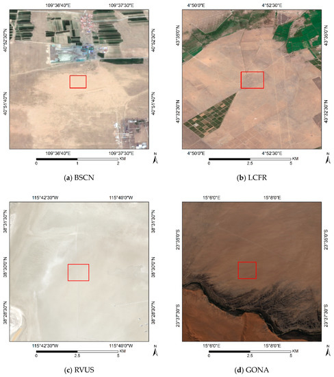
Figure 2.
Remote sensing images for four sites of RadCalNet with the ground core region indicated by the red square.
2.2. Satellite Observations and Site Measurements Overview
Google Earth Engine (GEE) platform and Python were selected as analysis tools because GEE is a cloud-based platform that can provide high-performance computing resources to process large geospatial datasets and enables access to global geospatial datasets [26].
2.2.1. Satellite Sensors
Sentinel-2 (S2) is a component of the European Space Agency’s Copernicus program and comprises two satellites: S2A, launched in June 2015, and S2B, launched in March 2017. S2A and S2B follow the same orbit but are separated by 180°, enabling a high revisit frequency of 5 d at the equator [27]. S2 features 13 spectral bands with a spatial resolution varying between 10 to 60 m. The width of the orbital swath is 290 km. The mean local solar time at the descending node is 10:30 a.m., near Landsat’s local overpass time [28]. L8 and S2A showed stable radiometric calibration with a consistency of ~2.5% [11]. A cross-comparison of S2A and S2B revealed a slight discrepancy of ~1%, though both satellites met the mission requirement for radiometric calibration accuracy of 3% [18,29,30].
The revolutionary Landsat series, the longest operating satellite series in orbit, was launched in July 1972. L8 OLI is the first choice when data in the region of interest (ROI) is incomplete. Although the scan line corrector in the Landsat 7 (L7) ETM+ failed in June 2003 and approximately 22% of the data are missing [31], the ROI is covered in satellite transit. The revisit period of L8 is 16 d with an equatorial crossing time of 10:00 a.m. ± 15 min [31]. After four years of on-orbit operation, the OLI is radiometrically stable at ~1.5% [32]. The stability of the absolute radiometric calibration of the OLI indicated that the instrument was within 5% radiance and 3% reflectance [33]. Although the SLC of L7 failed, these data still meet geometric and radiometric measurement accuracy [31]. ETM+ has demonstrated high radiometric stability within 2% based on PICS from 1999 to 2017 [12].
2.2.2. Site Data
The data provided by the RadCalNet, based on a reflectance-based approach within a verified uncertainty budget, are SI-traceable and used for the vicarious calibration of optical sensors ranging from visible to shortwave infrared wavelength [22,24]. The BOA reflectance data at a 10 nm spectral sampling interval combined with atmospheric parameters were processed to TOA reflectance using MODTRAN, and the uncertainty budgets of BOA and TOA were provided. Except for the temporal variability in the datasets of the PICS, the available wavelength range of the data also varies: the available band ranges for the BSCN are VNIR; for LCFR they are VNIR and SWIR; for RVUS they are VNIR and SWIR1; and for GONA they are VNIR and SWIR1. The RadCalNet provides nadir-view BOA reflectance data at 30 min intervals between 9 am and 3 pm local standard time.
Table 1 lists the time series of TOA (satellite) and BOA (site) reflectance data used in this study.

Table 1.
Time series range of BOA and TOA of RadCalNet.
The BOA data were used to verify the trends in the TOA data and assess the temporal stability of the RadCalNet for the first time. To ensure the accuracy of the results, the analyses controlled for cloud coverage in the transit site images and purified the time series TOA data for each site using the 1-sigma principle. The scaling factor of each sensor was adjusted to match the spectral response function of OLI, and the time series data of each site were corrected for the bidirectional reflectance distribution function (BRDF) to mitigate seasonal effects. Subsequently, the time series data were subjected to signal highlighting and drift correction based on uncertainty. Finally, the Mann–Kendall (MK) abrupt change test and MK trend analysis were applied to highlight short- and long-term trends time series data; Sen’s slope was used to quantify trend changes.
2.3. Cloud Filtering and Outlier Removal
To improve the representativeness of the data, 20% cloud cover was selected as a prerequisite for image collection. For S2, the QA band was selected to remove the cloudy pixels [34]. Likewise, the QA band was selected for Landsat, and the cloud removal method was the same as that for S2, both of which were based on bitmask. An empirical sigma (±1σ) filtering approach was used to remove outliers after removing cloud pixels. Visual image inspection was performed when the mean TOA reflectance of the ROI exceeded the threshold. If clouds, cloud shadows, or other artifacts were not identified within the ROI during the visual inspection, the scene of outliers was discarded from the analysis.
2.4. Scaling Adjustment Factor
An adjustment factor is required because the spectral response functions (SRF) vary between sensors (Figure 3), which can cause differences in reflectance and systematic errors [20]. The scaling adjustment factor (SAF) based on reflectance was employed to reduce the effects of sensor differences and adjust the sensors to the same scale [19,20,35]; the SAF can account for all types of differences between the “reference” and “adjustment” sensors with high accuracy, including SRF [19].
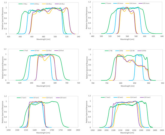
Figure 3.
Spectral response function for each band of ETM+, OLI, and MSI sensors (For the purpose of this article, only VNIR, SWIR1, and SWIR2 bands are displayed).
Given the temporal coverage of RadCalNet observation and superior radiometric performance, the OLI was chosen as the “reference” sensor, while the MSI and ETM+ were chosen as the “adjustment” sensors to match the OLI sensor by applying the SAF. The SAF was calculated as the mean of all ratios, that is, the mean of the ratio of the OLI TOA reflectance to near-coincident acquisitions with the OLI of each sensor. “Near-coincident acquisition” was carried out in the specified time window, with a time interval of 4 days between MSI and OLI, and 8 days between ETM+ and OLI. The SAF was calculated as follows:
where ρreference denotes the OLI TOA reflectance; ρadjustment denotes the MSI or ETM+ TOA reflectance; and n is the number of image pairs obtained from “near-coincident acquisition”.
2.5. BRDF-Adjusted Reflectance
TOA reflectance varies because of changes in solar and viewing geometry, especially in the longer wavelength bands because the Earth’s surface is non-Lambertian. To reduce the impact of solar and viewing angles, a four-angle BRDF empirical model was derived with minimal wavelength dependence [36]. In addition, a model with quadratic and interaction terms is well characterized and has better uncertainty after normalization [37]. The 15-coefficient quadratic model was used for this work to fit the TOA time series data from various angles to obtain the correction coefficient β. The normalized reflectance of each PICS at a specific angle was then determined.
where β0, β1, β2 … denotes the model coefficients; Y1, X1, Y2, and X2 are Cartesian coordinates representing the planar projections of the solar and sensor angles, which were originally given in the spherical coordinates:
where SZA, SAA, VZA, and VAA are the solar zenith, solar azimuth, view zenith, and view azimuth angles, respectively. The BRDF-normalized TOA reflectance was calculated as follows:
where ρobs is the observed mean TOA reflectance from the ROI of each scene; ρmodel is the model-predicted TOA reflectance; ρref is the TOA reflectance with respect to a set of “reference” solar and sensor position angles. For this analysis, the “reference” TOA reflectance is the average of the “combined” TOA data.
A practical BRDF model was used for normalizing the TOA reflectance with a set of angles, which is more reasonable than using a different BRDF model for the same site with different sensors [20]. As the site data were measured from the nadir (0° view zenith) of the instrument, the BOA reflectance was affected only by changes in the sun angle. Therefore, only the angle of the sun was linearly corrected.
2.6. Drift Corrections
Excluding the influence of the atmosphere and the non-Lambert surface, TOA data should show periodic changes with time. However, the degradation of the sensor itself, different atmospheric conditions, and the non-Lambertian nature of the site led to the introduction of different degrees of noise into the TOA data. Therefore, it is necessary to denoise the TOA data, expose the real information in the time series, and perform drift correction. Accordingly, the inverse variance-weighted average method was used as follows:
where ρi is the “combined” TOA reflectance time series, and wi is the weight determined by the inverse ratio of the square of the uncertainty of each point [38]. The moving window method was used to conduct the inverse-weighted average of the TOA, with a window size of 14 d due to the large data interval during the period when S2 was not operational. The total uncertainty (σtotal) comprised four parts of uncertainty: (1) spatial; (2) the BRDF model; (3) the SAF; (4) the sensor-calibration uncertainty. The σtotal is calculated as follows:
2.7. Temporal Stability Analysis
As some BRDF-corrected data bands do not follow the assumptions of normality and linearity, parametric tests may lead to misleading conclusions [19]. Nonparametric tests, such as the MK and sequential MK tests, are preferred because they are less affected by the overall distribution of the data. Hence, these tests were used for temporal stability analysis.
2.7.1. Sequential MK Test
The sequential version of the MK test is a nonparametric test that can detect potential trend turning points in long-term series data [39,40]. It has been used to detect abrupt changes in temperature and precipitation [41,42,43].
The sequential MK test is computed using the ranked values yi of the original values (x1, x2, x3, … xn), where forward u(t) and backward u’(t) sequential statistics were used to detect the points of change with magnitudes of yi (I = 1, 2, 3,… n) when compared with yj (j = 1, 2, 3,… i–1). For each comparison, the cases where yi > yj are counted and denoted by ni. The statistic ti is then calculated as
The distribution of test statistic ti, has a mean of
and variance of
The sequential values for the series were calculated for each test statistic variables ti as follows:
where u(ti) is a standardized variable that has a mean of zero and unit standard deviation, whose sequential behavior fluctuates around zero level [41]. While the forward sequential statistic u(t) is estimated using the original time series (x1, x2, x3, … xn), the backward sequential statistic u’(t) is estimated in the same way as u(t), but the estimation starts from the end of the series (xn, xn–1, xn–2, … x1). The intersection of the forward u(t) and backward u’(t) represents an approximate trend turning point. Abrupt change points are identified by the intersections of u(t) and u’(t) occurring outside the confidence level threshold of the standardized statistic. The threshold value in this study was ±1.96 (95% confidence level).
2.7.2. MK Test
The MK test is a rank-based nonparametric trend detection method that is widely used in time series analysis [44,45]. The test is based on two hypotheses: the null hypothesis H0, with non-monotonic trend data, and the alternative hypothesis H1, which follows a monotonic trend.
The MK test analyzes all potential pairs of measurements in the dataset to evaluate if a series of values trends upward or downward over time. The MK test statistic is calculated as follows:
where Xi and Xj are two variables from time series X; Xi represents (X1, X2, … Xi); and Xj represents (Xi+1, Xi+2, … Xj). If Xj is greater in magnitude than Xi, S increases by one; if Xj is less than Xi, S decreases by one. The sgn is defined as
The test was performed at a 0.05 significance level. An upward or downward trend is indicated by a positive or negative S value, respectively. The MK test not only detects the trend over the entire time series in every band, but also the trend in different periods separated by change points detected using the sequential MK test.
2.7.3. Sen’s Slope Estimator
Sen’s slope statistic is a nonparametric test proposed by Sen [46]. Strong fitting of Sen’s slope results in a more robust slope estimate than the least-squares approach [46]. For this purpose, Sen’s slope was selected to estimate the slope of the trend in the entire time series for each segment, which is calculated as follows:
where k = [1, N(N–1)/2, i = [1, N–1], and j = [2, N] which ensures that i < j. Qk indicates the slope of a data pair. Sen’s slope is then calculated as the median of all slopes (Qk):
Hence, Qmed represents the time series data’s trend and slope, which are related to the MK (represented by S) test [47]. The confidence interval of Qmed was obtained under a particular probability to ascertain whether the median slope was statistically significant. The confidence interval of the slope is given by
where Z1–α/2 was obtained from a common normal distribution table.
Var (S) and Zs are computed as follows:
where n is the number of data series, m the number of tied groups (the same value is a tied group), and ti is the number of data series in the i-th group.
2.8. Spatial Homogeneity Analysis
The spatial homogeneity of the site is the basis of radiometric calibration. CV and Gi* represent the site’s local variability and spatial clustering, respectively. CV and Gi* are suitable combinations for screening spatial homogeneity regions [4]. Hence, CV and Gi* were used for spatial homogeneity analysis.
CV is a dimensionless value that provides a standardized measure of reflectance variability within a defined area of an image. The CV has been widely used to estimate spatial homogeneity of vicarious calibration sites [4,7,48,49]. The CV is defined as follows:
where σ and x are the standard deviation and mean within a pre-defined window, respectively. For Landsat, the 3 3 window is selected, and S2 is 9 9 to match the difference in resolution.
The Gi* statistic, which gives a measure of clustering, is a local indicator of spatial association, indicating spatial homogeneity and dependence when similar values are clustered [50,51]. The Gi* is defined as follows:
where n is the total number of pixels; x is the global mean of x; s is the variance of x; wij(d) is a matrix of spectral weights with binary and symmetric weight equal to unity (wij = 1) for all pixels found within the distance d of pixel i considered and a weight equal to zero (wij = 0) for all pixels found outside d; ∑wij(d)xj is the sum of varying values X within the distance d of pixel I; W*i is the number of pixels within the distance d. Gi* values greater than zero were extracted, indicating spatial homogeneity of the matrix region; the region consists of the same kind of elements or has a similar nature in space, meaning that it exhibits a similar spatial reflectance structure [4,52].
3. Results
3.1. Statistical Analysis of GONA
3.1.1. Scaling Adjustment
The TOA distribution of each sensor without adjustment is shown in Figure 4. Figure 5 shows the “virtual constellation” combining the sensor data [53] after the SAF adjustment. Comparison of sensor data before and after adjustment showed that the SAF had a minor adjustment on the reflectance of S2 and L7, particularly for bands with shorter wavelengths. However, the adjustment effect was more pronounced for bands with longer wavelengths. This is because of the low reflectance energy in shorter wavelength bands; the reflectance energy fluctuates significantly with the increase in wavelength [14]. Additionally, the SRF between the sensors did not differ significantly in the shorter wavelength bands. Consequently, the “fit” of the S2, L7, and L8 reflectance data was already near perfect in the shorter wavelength bands before the SAF adjustment. The obvious offsets of the longer wavelength may be due to the overall effect of the spectral energy characteristics of longer wavelengths, RSR difference, and the atmospheric effect [14]. The SAF not only adjusts the difference between sensors, but also equalizes the influence of the atmosphere [19].


Figure 4.
TOA reflectance before SAF adjustment of the combined data.
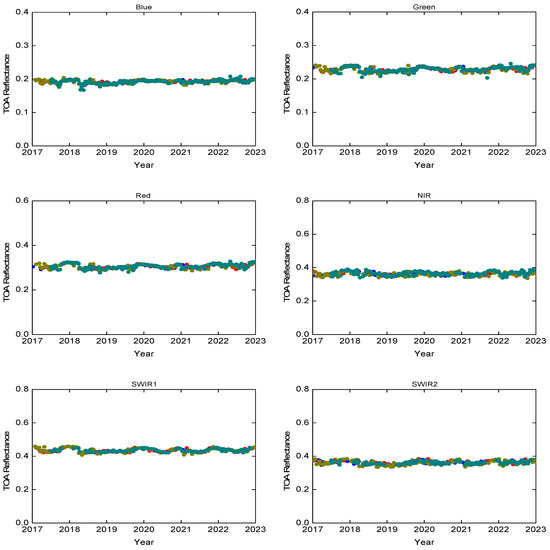

Figure 5.
TOA reflectance after SAF adjustment of the combined data.
3.1.2. BRDF Correction
Figure 6 shows the BRDF-corrected TOA reflectance. The BRDF (based on 15 coefficient-corrected GONA datasets) reduced directional effects. It can be seen from the figure that BRDF correction seems to play little role, and only fine-tuned the raw TOA data. This is because the surface type of GONA has the minimum BRDF effect, and the terrain is relatively flat [24]. For SWIR1 and SWIR2 bands, the model was proved to be effective. The temporal trends among the bands remained consistent before and after the correction, indicating consistency for each band response of the sensor on GONA. Table S1 lists the β-parameter values of the BRDF model for each band of the four PICS in RadCalNet.
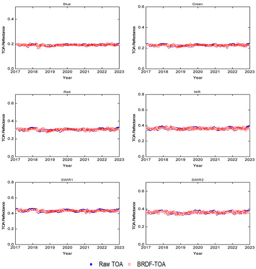
Figure 6.
TOA reflectance after BRDF correction of GONA.
3.1.3. Drift Correction
Figure 7 shows that the distribution of TOA data was evened out after weight adjustment. However, some time node data are distinct from the overall distribution because of a limited amount of data, which impedes the accurate analysis of trends in the data. Data distribution has large changes that were not removed because they represent trends in the dataset. Overall, there were no obvious fluctuations in the dataset, reflecting the long-term trends in the data. Table 2 lists the total uncertainties of the four data sources.
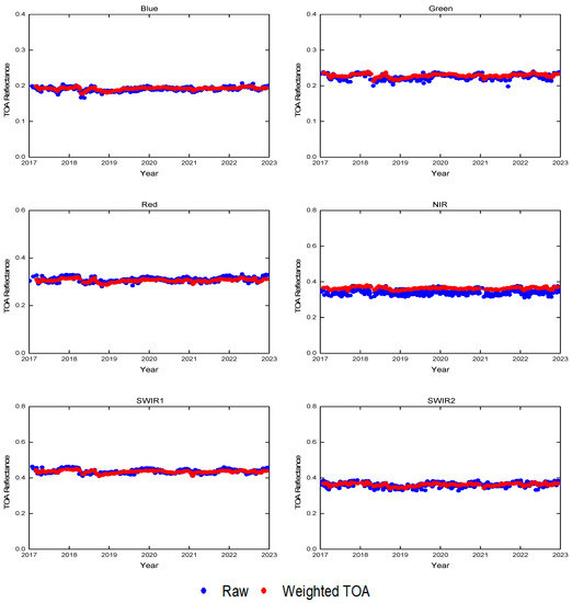
Figure 7.
TOA reflectance after weight adjustment of the combined data of GONA.
Table 2.
Total average uncertainty of RadCalNet.
3.1.4. Sequential MK Analysis for TOA and BOA Data
The sequential MK test was conducted for the GONA dataset at a 95% confidence level using a critical value of ±1.96. The intersection points of the curve indicate statistically significant changes in the yearly trend of the TOA. Figure 8 shows the sequential MK trend analysis for the TOA series of GONA. For all bands, except the NIR and SWIR2 bands, an abrupt change point occurred in 2021; however, only the SWIR1 band was within the confidence interval, which proved that this abrupt change point was statistically significant. All bands’ forward and backward trends were roughly the same, indicating good consistency in their radiometric performance at this site. The NIR and SWIR1 bands had two abrupt change points in 2017 and 2018, but a statistically significant change was detected only in 2018. In 2022, multiple change points occurred in the NIR, SWIR1, and SWIR2 bands, but only the change point in the NIR band was significant. Table 3 presents the years of significant change points in each band.
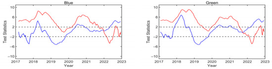
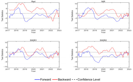
Figure 8.
Test of abrupt change points for the combined TOA data of GONA.
Table 3.
Change point detection using sequential MK test for TOA data of GONA (* p ≤ 0.05).
Figure 9 shows the sequential MK trend analysis for the yearly BOA data of GONA. The BOA data were first filtered by an aerosol optical depth (AOD) of less than 0.2, corrected by the BRDF, and finally weighted by the inverse variance of the uncertainties. The uncertainties include the residual of the BRDF model and the uncertainty of wavelength reflectance. SWIR2 was not calculated because the wavelength range of the GONA instrument could not support the complete calculation of reflectance. The positive sequential MK curve of each band showed a high degree of consistency, consistent with the reverse curve. This reflects the homogeneity of the site reflectance at each wavelength. All bands, except for the NIR band, exhibited a statistically significant abrupt change in 2021 (2022 for the NIR band). Table 4 presents the years of significant change points for each band.
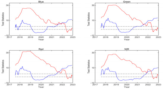
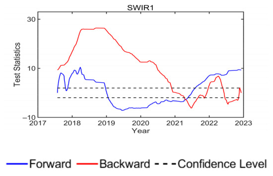
Figure 9.
Test of abrupt change points for the combined BOA data of GONA.
Table 4.
Change point detection using the sequential MK test for BOA data of GONA (* p ≤ 0.05).
Comparison of the sequential MK tests of the TOA and BOA datasets revealed that the abrupt change points reflected by the TOA did not necessarily correspond with changes in the BOA data. This may be related to the impact of the atmosphere, as the optical path containing the actual surface information may be masked or obscured by atmospheric effects. In addition, the spectral band adjustment adjusts the atmospheric condition of the image to the atmospheric state of a scene or the average atmospheric state of multi-scene images, which will further mask the real surface state.
3.1.5. MK Trend and Sen’s Slope Estimator Analysis for TOA and BOA Data
The MK trend test was applied to the combined data to determine long-term trends for GONA’s TOA and BOA datasets (Table 5). The test results showed a long-term monotonic trend for all bands of the BOA data; only the blue, green, and red had a long-term monotonic trend for the TOA data. The MK test of the BOA showed a strong significance level. For the NIR, SWIR1, and SWIR2 bands of TOA, there was insufficient evidence for a monotonic trend, which means that these bands were stable during the entire period; however, Sen’s slope provides a monotonic trend without a significant level to support this evidence. These analyses provide sufficient evidence to support a monotonic trend for the five bands of the BOA data and three bands in the TOA data. This inconsistency between the datasets proves that the surface information reflected in the TOA data is affected by atmospheric and spectral band adjustments.
Table 5.
MK trend test and Sen’s slope for TOA and BOA data of GONA (at 0.05 significance level).
Table 6 lists the MK test and Sen’s slopes results for each abrupt change point in the TOA and BOA data, respectively. No statistically significant abrupt change points were found in the blue, green, red, or SWIR2 bands. Instead, significant abrupt change points were observed in the NIR and SWIR1 bands, where data on both sides of the NIR band showed an increasing trend. Specifically, a significant increasing trend in the SWIR1 band was detected between 2017 and 2018, followed by a downward trend from 2021 to 2022. There was insufficient statistical evidence to support a monotonic trend from 2018 to 2021; although the slope indicated a possible increase outside the confidence interval, it exceeded outside the significance level. With the exception of the SWIR1 band, an increasing trend was detected in each abrupt change interval of the other four bands of the BOA data, coinciding with each band’s overall trend. The two abrupt change intervals of the SWIR1 band showed a decreasing trend and an overall upward trend, which may be difficult to understand intuitively, but was consistent with the statistical analysis.
Table 6.
MK trend test and Sen’s slope for each change point for TOA and BOA data of GONA (at 0.05 significance level).
3.2. Statistical Analysis of BSCN, RVUS, and LCFR
The previous section summarized the results for GONA and illustrated our step-by-step analytical procedure. The results for BSCN, RVUS, and LCFR are presented in this section, with all tests conducted at a 95% confidence level. The number of bands of BOA data at each site is based on the wavelength ranges provided by the sites.
Figure 10 and Figure 11 present the sequential MK test results for the TOA and BOA data of BSCN, respectively. The forward and backward sequential MK test curves of each band showed strong consistency. Consequently, it can be inferred that the site was similar in the long time series TOA and BOA trends of the visible, NIR, and SWIR bands. Although the curves intersected, not all intersections represented turning points because they were not statistically significant. Except for the blue and SWIR2 bands, all other bands in the TOA time series had significant abrupt turning points in 2019. Actual change points for the red and NIR bands occurred in 2021 and 2018, respectively. The only significant abrupt point in the blue band was in 2020. The actual change point in the SWIR2 band only occurred in 2021. Compared with the BOA time series data, only the blue and green bands changed significantly in 2020, while the red and NIR bands had several intersections, but both exceeded the confidence range. Table 7 and Table 8 list the change points detected by using the sequential MK test for the TOA and BOA data of BSCN, respectively.
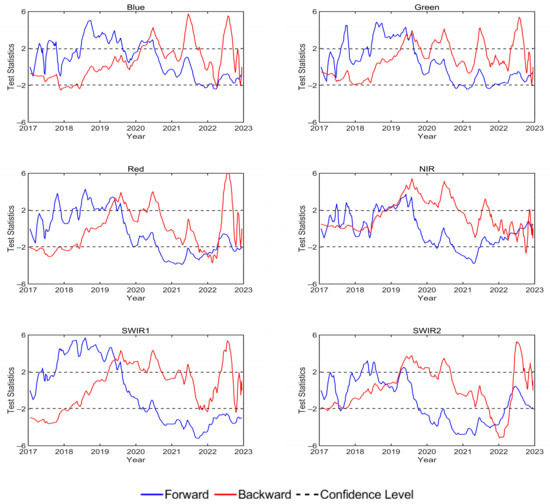
Figure 10.
Test of abrupt change points for the combined TOA data of BSCN.


Figure 11.
Test of abrupt change points for the combined BOA data of BSCN.
Table 7.
Change points detected using the sequential MK test for TOA data of BSCN (* p ≤ 0.05).
Table 8.
Change points detected using the sequential MK test for BOA data of BSCN (* p ≤ 0.05).
Table 9 lists the MK trend test and Sen’s slope results for each change point of the TOA and BOA data of BSCN. The results showed an increasing trend in each abrupt change interval for each band of the TOA data, except for the red band from 2021 to 2022 and each abrupt change region of the SWIR2 band. Additionally, there was a long-term increasing trend across each abrupt change interval of the blue and green bands for the BOA data.
Table 9.
MK trend test and Sen’s slope of each change point for TOA and BOA data of BSCN (at 0.05 significance level).
Figure 12 and Figure 13 show the sequential MK test results for the TOA and BOA data of RVUS, respectively. A significant abrupt change point for each band of the TOA data was detected in 2022, while the abrupt change points of the BOA occurred in 2020, 2021, and 2022. The abrupt points of each band in 2020 and 2022 were significant within the confidence interval. In 2021, the other abrupt change points of bands were statistically significant, except for the blue, green, and red bands. Table 10 and Table 11 list the change points detected by using the sequential MK test for the TOA and BOA data of RVUS, respectively.

Figure 12.
Test of abrupt change points for the combined TOA data of RVUS.
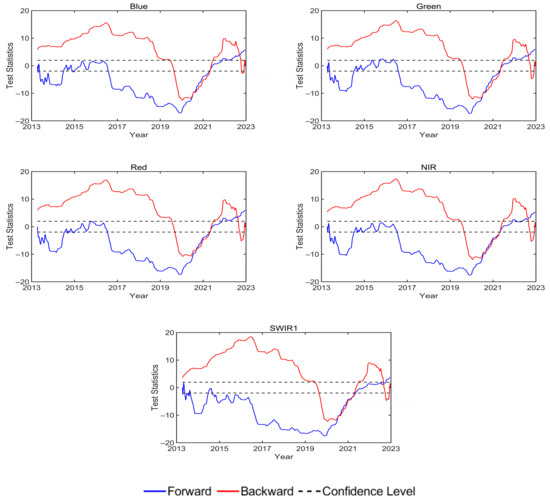
Figure 13.
Test of abrupt change points for the combined BOA data of RVUS.
Table 10.
Change points detected using the sequential MK test for TOA data of RVUS (* p ≤ 0.05).
Table 11.
Change points detected using the sequential MK test for BOA data of RVUS (* p ≤ 0.05).
Table 12 lists the MK trend test and Sen’s slope results of each abrupt change point for the TOA and BOA data of RVUS. A clear increasing trend was found for each abrupt change interval in each band of the TOA data. For the BOA data, all abrupt change intervals showed a significant downward trend from 2020 to 2021, except for those in the NIR and SWIR1 bands. The NIR band exhibited no statistically significant trend change between 2020 and 2021, while SWIR1 showed an increasing trend.
Table 12.
MK trend test and Sen’s slope of each change point for TOA data of RVUS (at 0.05 significance level).
It is significant to note that the LCFR site’s surface varies from moderate vegetation and pebble cover in the winter and spring to a semi-arid soil surface in the summer and fall [54,55]. For improved accuracy in the results, the TOA and BOA data of the LCFR site were separated by seasons, with winter and spring in one group and summer and autumn in another group.
Figure 14 and Figure 15 show the sequential MK test results for the TOA and BOA data of LCFR (winter and spring), respectively. An abrupt change point was observed in 2019 for all bands except the blue band in 2020 and the NIR band in 2021, with only the blue and red bands being statistically significant. For the SWIR1 and SWIR2 bands, the change points were detected in 2016, 2019, and 2022. However, the probability values were below the 95% confidence level and could not be utilized as significant change points. For the BOA data, multiple abrupt change points were detected in each band. Except for the SWIR band, there are significant abrupt points in all other bands between 2015 and 2022, with the blue band in 2017, 2018, and 2019, the green band in 2015 and 2020, the red band in 2017 and 2020, and the NIR band in 2019 and 2020. The SWIR bands were all detected with change points in 2017, but not significantly. Table 13 and Table 14 list the change points detected using the sequential MK test for the TOA and BOA data of LCFR (winter and spring), respectively.
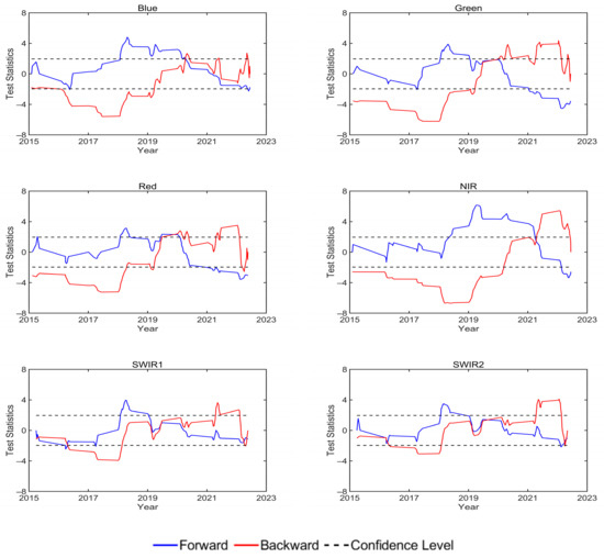
Figure 14.
Test of abrupt change points for the combined TOA data of LCFR (winter and spring).
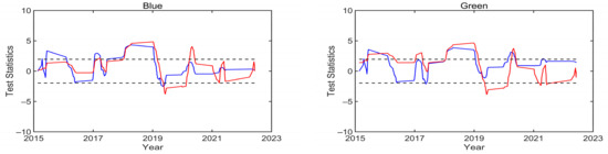

Figure 15.
Test of abrupt change points for the combined BOA data of LCFR (winter and spring).
Table 13.
Change points detected using the sequential MK test for TOA data of LCFR (winter and spring) (* p ≤ 0.05).
Table 14.
Change points detected using the sequential MK test for BOA data of LCFR (winter and spring) (* p ≤ 0.05).
Table 15 lists the MK trend test and Sen’s slope results of each abrupt point for the TOA and BOA data of LCFR (winter and spring). A monotonic trend was detected in all bands of each abrupt interval of the TOA and BOA data, except for the blue band from 2015 to 2017 of the BOA data. In addition, the trends and abrupt change intervals varied between the TOA and BOA data. An increasing trend was detected in the red and green bands of the TOA at various abrupt intervals, and the magnitude of the slope was lower than 10 × 10−4. For the BOA data, a statistically significant change was not detected in the blue band between 2015 and 2017, with a monotonically increasing trend between 2017 and 2018 and 2018 and 2019, and a downward trend between 2019 and 2022. There was a significant increase in the green and red bands at each abrupt interval. A downward trend was detected between 2015 and 2019 for the NIR band, but it monotonically increased within the two abrupt intervals of 2020 and 2022.
Table 15.
MK trend test and Sen’s slope of each change point for TOA and BOA data of LCFR (winter and spring) (at 0.05 significance level).
Figure 16 and Figure 17 show the sequential MK test results for the TOA and BOA data of LCFR (summer and autumn), respectively. For TOA data, an abrupt change point was found in all bands, except for the blue and SWIR2 bands in 2020, where only NIR was statistically significant. An actual change point was detected in the blue band in 2016 and 2019. In 2022, a significant abrupt change point was detected in the green and SWIR2 bands. For the BOA data, multiple abrupt change points were detected in all bands, some of which were statistically significant. The abrupt points of the green band in 2015, the red band in 2015 and 2019, the NIR band in 2016, and the two SWIR bands in 2016, 2019, and 2020 are all reliable at the confidence levels. Table 16 and Table 17 list all the detected change points.
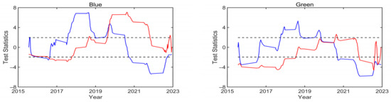
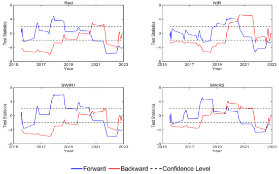
Figure 16.
Test of abrupt change points for the combined TOA data of LCFR (summer and autumn).
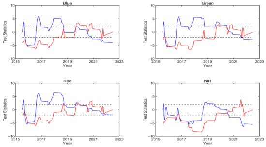

Figure 17.
Test of abrupt change points for the combined BOA data of LCFR (summer and autumn).
Table 16.
Change points detected using the sequential MK test for TOA data of LCFR (summer and autumn) (* p ≤ 0.05).
Table 17.
Change points detected using the sequential MK test for BOA data of LCFR (summer and autumn) (* p ≤ 0.05).
Table 18 lists the MK trend test and Sen’s slope results of each abrupt change point for the TOA and BOA data of LCFR (summer and autumn). The blue band of the TOA was detected with a downward trend from 2015 to 2016 and an increase from 2016 to 2019 and also from 2019 to 2022. However, there is no abrupt interval in the blue band of the BOA at the confidence level. The red band of the BOA was detected with a monotonic increase between 2019 and 2022, but no abrupt interval was detected in the red band of the TOA. The green and SWIR2 bands of the TOA were detected decreasing between 2015 and 2022, while the NIR band increased at various intervals. A downward trend was detected in the NIR band of the BOA within the abrupt interval. There is an increasing trend in the SWIR1 band between 2020 and 2022, but no statistically significant trend was detected in other intervals. The SWIR2 band was detected decreasing and increasing from 2015 to 2016 and 2020 to 2022, respectively. It can be found that the TOA and BOA data showed different trends and abrupt change intervals.
Table 18.
MK trend test and Sen’s slope of each change point for TOA and BOA data of LCFR (summer and autumn) (at 0.05 significance level).
Table 19 lists the MK trend test and Sen’s slope results for the TOA and BOA data of the BSCN, RVUS, and LCFR sites over the study period. All bands for the TOA data of RVUS showed a significant long-term upward trend. Compared with the BOA data, there was a long-term upward trend within the significance level. For the TOA data of BSCN, all bands, except for the red and SWIR1 bands, were temporally stable. In contrast, the BOA data of BSCN lacked enough evidence to prove the monotonicity of all bands. For the TOA data of LCFR (winter and spring), the green, red, and NIR bands showed a significant long-term downward trend across the entire period, while the other three bands were temporally stable. For the BOA data of LCFR (winter and spring), an increasing trend was detected in only the SWIR1 and SWIR2 bands, while the other bands were temporally stable. For TOA data of LCFR (summer and autumn), there was a downward trend for all bands except for the blue band, while the BOA data showed a long-term downward trend in all bands except for the red, SWIR1, and SWIR2 bands.
Table 19.
MK trend test and Sen’s slope for TOA and BOA data of BSCN, RVUS, and LCFR (at 0.05 significance level, * indicates instances where the reflectance of the corresponding wavelength was not provided).
3.3. Percentage Change from the TOA and BOA of the RadCalNet That Reflects Instability and Indicates That This Site Cannot Be Used to Reliably Track the Radiometric Performance of the SWIR1 and SWIR2 Bands
Table 20 lists the percentage change of the RadCalNet for the study period. It can be seen that the TOA and BOA datasets varied in the degree of change. The change in trend for the TOA data was significantly smaller than that for the BOA data, except for RVUS. This discrepancy may be attributed to the atmosphere’s influence and the sensor’s attenuation uncertainty. While the uncertainties in the BRDF and SAF models, sites, and sensors had been considered and corrected, the uncertainty of the satellite sensor was taken as a constant value. In fact, the uncertainty of the sensor is continually changing. Overall, BSCN exhibited good stability, based on both the TOA and BOA data. However, the annual percentage change of the SWIR1 and SWIR2 bands of LCFR reached 1.144% and 1.803%, respectively, which reflects instability and indicates that this site cannot be used to reliably track the radiometric performance of the SWIR1 and SWIR2 bands.
Table 20.
Annual percentage change in TOA and BOA data over the study period (- represents insufficient evidence to support monotonous trends. * indicates instances where the reflectance of the corresponding wavelength range was not provided by the site instrument).
3.4. Spatial Stability Analysis of RadCalNet
Table 21 lists the ratio of site homogeneity reaching the standard during the operation period of each site. Whether it is local variability or spatial clustering, the proportion of GONA bands meeting the conditions was greater than 0.979, and the ratio of the blue and green bands meeting the local variability conditions reached 1. GONA exhibits very good spatial homogeneity throughout the year [56]. The other three sites also basically met the spatial homogeneity conditions during the satellite transit, with the lowest spatial clustering ratio of 0.582 found in the NIR band of LCFR. This suggests that the NIR band of LCFR was homogeneous only half of the time throughout the year, which is reasonable considering the seasonal variation in the surface type of LCFR [54,55]. The NIR band exhibits spatial heterogeneity when the local surface is a mixture of cobbles and sparse vegetation.
Table 21.
Ratio of CV and Gi meeting conditions at each site of RadCalNet during the operation (The condition of CV is less than 3%, and of Gi* greater than 0).
4. Discussion
Tuli [19] and Khadka [20] used multi-sensor TOA data (ETM+, OLI, MSI, and MODIS) to evaluate the temporal stability of the six PICS used by the SDSU for calibration analysis. However, it is important to note that atmospheric conditions can easily affect the TOA data, which may not accurately reflect true surface information. Therefore, when analyzing and evaluating the temporal stability of PICS sites using TOA data, the authenticity of the results should be considered and discussed. This study focused on evaluating the RadCalNet sites and aimed to verify the authenticity of the surface reflected by the sequence of the TOA data. The BOA data were obtained using strict criteria, including an AOD of less than 0.2 and a consideration of uncertainty, to ensure the reliability of the results.
The analyses of this study showed that the TOA and BOA data varied in terms of significant abrupt change points and trends, indicating that the real change state of the PICS surface cannot be accurately reflected using long-term TOA data. This is likely because the atmosphere alters the optical path containing the surface information before it reaches the satellite sensor. Therefore, the TOA data contain both surface and atmospheric information. The discrepancy could also be related to the spectral band adjustment. The SAF was obtained from the mean ratio of the image values closest to the two sensors. This can alter the RSR and other differences between the two sensors [19], meaning that the atmospheric state of all images is adjusted to the average atmospheric state of the near-coincident acquisition image pair. The surface reflectance noise in the data and spectral band adjustment can obscure the real surface information and lead to misinterpretations. Compared to the multi-satellite sensor data of Tuli and Khadka, this experiment only used data from ETM+, OLI, and MSI sensors owing to the size limitation of the site’s core area, resulting in a disadvantage in temporal resolution.
The interpretation of our results was supported by a high level of confidence and statistical significance based on the MK test and Sen’s slope. As shown, it reflects instability and indicates that this site cannot be used to reliably track the radiometric performance of the SWIR1 and SWIR2 bands.
As can be seen in Table 20, for some bands, such as the visible light bands of BSCN and LCFR (winter and spring) and the red SWIR1 and SWIR2 bands of LCFR (winter and spring), there is insufficient evidence to support the monotonous trends of abrupt change intervals outside the confidence level, indicating that the bands are stable. However, the annual change rates of the green band of GONA, the blue band of LCFR (summer and autumn), and the SWIR1 and SWIR2 bands of LCFR (winter and spring) all exceeded 1%, surpassing the radiometric accuracy of sensor-traceable radiometry underpinning terrestrial and helio studies (0.3%) [57]. This indicates that these bands are unstable at these sites and unsuitable for monitoring the sensors’ radiometric performance. Moreover, the magnitude of change of these bands within the operating period (>5%) is greater than the task requirements of OLI, ETM+, and MSI sensor calibration uncertainties (5% for ETM+ and 3% for OLI and MSI), which further proves that the site cannot be used as a radiometric performance tracking source. While the long-term reflectance shows a significant rate of change (0.282%/year–1.324%/year) at the confidence level, the CV remains essentially less than 3% and the Gi* greater than 0 (Table 21), indicating that the RadCalNet is homogenous enough for use in radiometric calibration. Nonetheless, using the sites with the large change rates for radiometric performance tracking of the corresponding bands would be inappropriate and likely to result in errors.
The trend analysis of the RadCalNet sites provides an uncertainty basis for satellite sensor calibration. The BOA data could effectively reveal the changes in reflectance trends between bands at each site determined using TOA data and quantify spatial stability and temporal instability at the RadCalNet sites. Our study can provide reference for researchers who use the TOA to quantify PICS radiometric stability and for satellite calibration and radiometric performance tracking using the RadCalNet sites.
5. Conclusions
The monitoring of sensor performance is closely related to data quality and accuracy, and PICS-based calibration has become the most popular method for monitoring sensor radiometric performance. However, previous studies had confirmed that PICS are not temporally stable, but the results were performed using TOA data without the support of surface reflectance data. Therefore, this study analyzed the spatiotemporal stability of the RadCalNet sites (for the GONA, BSCN, RVUS, and LCFR) using three sensors (ETM+, OLI, and MSI) and site BOA data, while also verifying the accuracy of the surface state reflected in the TOA time series. Additionally, it provides the first comprehensive evaluation of the temporal stability of RadCalNet, estimates the magnitude of change using the more robust Sen’s slope, and serves as a useful reference for sensor calibration and radiometric performance monitoring. The results showed that (1) the TOA time series data cannot accurately reflect the real change points and long-/short-term trends of the surface compared to the BOA data. Significant abrupt changes were detected in each band for the TOA data of RUVS in 2022, with each abrupt change interval exhibiting an increasing trend; however, the abrupt changes detected in each band of the BOA data occurred in 2020 and showed a downward trend. (2) Based on the analysis of the BOA data, it was found that the RadCalNet sites exhibited a monotonic trend and a significant annual change rate since the initiation of its operation. Each band of GONA, RVUS, and LCFR showed an annual rate of change > 0.2%, with a maximum of 1.803%. However, for BSCN, there was insufficient evidence to support a monotonous trend. (3) Nevertheless, our findings support the applicability of the RadCalNet for calibration based on the CV and Gi statistics for each site.
This study provides a verification reference for using the TOA to evaluate the accuracy of PICS spatiotemporal stability. Moreover, it proposes the use of the more robust Sen’s slope to characterize site trends. Although the change in reflectance trends based on the TOA data did not completely match that based on the BOA data, the RadCalNet sites showed good radiometric calibration performance. To improve the accuracy of reflectance estimated using the TOA data, future studies would benefit from a more precise characterization of atmospheric conditions and the replacement of the SAF with SBAF for more accurate fusion.
Supplementary Materials
The following supporting information can be downloaded at: https://www.mdpi.com/article/10.3390/rs15102639/s1, Table S1: β-parameter values of BRDF model for each band of the four sites in RadCalNet.
Author Contributions
Conceptualization, H.Z. and E.Q.; methodology, E.Q.; investigation, E.Q., Z.C. and C.Z.; data curation, E.Q.; formal analysis, H.Z. and C.M.; validation, E.Q.; writing—original draft preparation, E.Q.; writing—review and editing, H.Z.; project administration, H.Z. and C.M. All authors have read and agreed to the published version of the manuscript.
Funding
This work has been supported by the National Natural Science Foundation of China (Grant No. U21A20108), the National Natural Science Foundation of China (Grant No. 41771397 and No. 42071330), and the Major Project of High Resolution Earth Observation System (Grant No. 30-Y60B01-9003-22/23).
Data Availability Statement
Not applicable.
Conflicts of Interest
The authors declare no conflict of interest.
References
- Shrestha, M.; Leigh, L.; Helder, D. Classification of North Africa for Use as an Extended Pseudo Invariant Calibration Sites (EPICS) for Radiometric Calibration and Stability Monitoring of Optical Satellite Sensors. Remote Sens. 2019, 11, 875. [Google Scholar] [CrossRef]
- Mishra, N.; Helder, D.; Angal, A.; Choi, J.; Xiong, X. Absolute Calibration of Optical Satellite Sensors Using Libya 4 Pseudo Invariant Calibration Site. Remote Sens. 2014, 6, 1327–1346. [Google Scholar] [CrossRef]
- Teillet, P.; Chander, G. Terrestrial reference standard sites for postlaunch sensor calibration. Can. J. Remote Sens. 2010, 36, 437–450. [Google Scholar] [CrossRef]
- Odongo, V.; Hamm, N.; Milton, E. Spatio-Temporal Assessment of Tuz Gölü, Turkey as a Potential Radiometric Vicarious Calibration Site. Remote Sens. 2014, 6, 2494–2513. [Google Scholar] [CrossRef]
- Cosnefroy, H.; Leroy, M.; Briottet, X. Selection and characterization of Saharan and Arabian desert sites for the calibration of optical satellite sensors. Remote Sens. Environ. 1996, 58, 101–114. [Google Scholar] [CrossRef]
- Ling, W.; Xiuqing, H.; Yupeng, L.; Zhizhao, L.; Min, M. Selection and Characterization of Glaciers on the Tibetan Plateau as Potential Pseudoinvariant Calibration Sites. IEEE J. Sel. Top. Appl. Earth Obs. Remote Sens. 2019, 12, 424–436. [Google Scholar] [CrossRef]
- Bannari, A.; Omari, K.; Teillet, P.M.; Fedosejevs, G. Potential of Getis statistics to characterize the radiometric uniformity and stability of test sites used for the calibration of Earth observation sensors. IEEE Trans. Geosci. Remote Sens. 2005, 43, 2918–2926. [Google Scholar] [CrossRef]
- Helder, D.L.; Basnet, B.; Morstad, D.L. Optimized identification of worldwide radiometric pseudo-invariant calibration sites. Can. J. Remote Sens. 2010, 36, 527–539. [Google Scholar] [CrossRef]
- Mitchell, R.M.; O’Brien, D.M.; Edwards, M.; Elsum, C.C.; Graetz, R.D. Selection and Initial Characterization of a Bright Calibration Site in the Strzelecki Desert, South Australia. Can. J. Remote Sens. 2014, 23, 342–353. [Google Scholar] [CrossRef]
- Kim, W.; He, T.; Wang, D.; Cao, C.; Liang, S. Assessment of long-term sensor radiometric degradation using time series analysis. IEEE Trans. Geosci. Remote Sens. 2013, 52, 2960–2976. [Google Scholar] [CrossRef]
- Barsi, J.A.; Alhammoud, B.; Czapla-Myers, J.; Gascon, F.; Haque, M.O.; Kaewmanee, M.; Leigh, L.; Markham, B.L. Sentinel-2A MSI and Landsat-8 OLI radiometric cross comparison over desert sites. Eur. J. Remote Sens. 2018, 51, 822–837. [Google Scholar] [CrossRef]
- Micijevic, E.; Mishra, N.; Helder, D. Assessing Long Term Stability of Landsat 5 TM, Landsat 7 ETM+ and Landsat 8 OLI. In Proceedings of the Conference on Characterization and Radiometric Calibration for Remote Sensing (CALCON), Logan, UT, USA, 21–24 August 2017. [Google Scholar]
- Doelling, D.R.; Wu, A.; Xiong, X.; Scarino, B.R.; Bhatt, R.; Haney, C.O.; Gopalan, A. The radiometric stability and scaling of collection 6 Terra-and Aqua-MODIS VIS, NIR, and SWIR spectral bands. IEEE Trans. Geosci. Remote Sens. 2015, 53, 4520–4535. [Google Scholar] [CrossRef]
- Chander, G.; Xiong, X.; Choi, T.; Angal, A. Monitoring on-orbit calibration stability of the Terra MODIS and Landsat 7 ETM+ sensors using pseudo-invariant test sites. Remote Sens. Environ. 2010, 114, 925–939. [Google Scholar] [CrossRef]
- Barsi, J.A.; Markham, B.L.; Helder, D.L. Continued monitoring of Landsat reflective band calibration using pseudo-invariant calibration sites. In Proceedings of the 2012 IEEE International Geoscience and Remote Sensing Symposium, Munich, Germany, 22–27 July 2012. [Google Scholar]
- Liu, Y.; Ma, L.; Wang, N.; Qian, Y.; Qiu, S.; Li, C. Vicarious radiometric calibration/validation of Landsat-8 operational land imager using a ground reflected radiance-based approach with Baotou site in China. J. Appl. Remote Sens. 2017, 11, 044004. [Google Scholar] [CrossRef]
- Tonooka, H.; Sakai, M.; Kumeta, A.; Nakau, K. In-Flight Radiometric Calibration of Compact Infrared Camera (CIRC) Instruments Onboard ALOS-2 Satellite and International Space Station. Remote Sens. 2019, 12, 58. [Google Scholar] [CrossRef]
- Revel, C.; Lonjou, V.; Marcq, S.; Desjardins, C.; Fougnie, B.; Coppolani-Delle Luche, C.; Guilleminot, N.; Lacamp, A.-S.; Lourme, E.; Miquel, C. Sentinel-2A and 2B absolute calibration monitoring. Eur. J. Remote Sens. 2019, 52, 122–137. [Google Scholar] [CrossRef]
- Tuli, F.T.Z.; Pinto, C.T.; Angal, A.; Xiong, X.; Helder, D. New Approach for Temporal Stability Evaluation of Pseudo-Invariant Calibration Sites (PICS). Remote Sens. 2019, 11, 1502. [Google Scholar] [CrossRef]
- Khadka, N.; Teixeira Pinto, C.; Leigh, L. Detection of Change Points in Pseudo-Invariant Calibration Sites Time Series Using Multi-Sensor Satellite Imagery. Remote Sens. 2021, 13, 2079. [Google Scholar] [CrossRef]
- Jing, X.; Uprety, S.; Liu, T.-C.; Zhang, B.; Shao, X. Evaluation of SNPP and NOAA-20 VIIRS Datasets Using RadCalNet and Landsat 8/OLI Data. Remote Sens. 2022, 14, 3913. [Google Scholar] [CrossRef]
- Bouvet, M.; Thome, K.; Berthelot, B.; Bialek, A.; Czapla-Myers, J.; Fox, N.; Goryl, P.; Henry, P.; Ma, L.; Marcq, S.; et al. RadCalNet: A Radiometric Calibration Network for Earth Observing Imagers Operating in the Visible to Shortwave Infrared Spectral Range. Remote Sens. 2019, 11, 2401. [Google Scholar] [CrossRef]
- USGS. EROS Cal/Val Center of Excellence. Available online: https://calval.cr.usgs.gov/apps/test_sites_catalog (accessed on 10 March 2023).
- Shrestha, M.; Helder, D.; Christopherson, J. DLR Earth Sensing Imaging Spectrometer (DESIS) Level 1 Product Evaluation Using RadCalNet Measurements. Remote Sens. 2021, 13, 2420. [Google Scholar] [CrossRef]
- Jing, X.; Leigh, L.M.; Pinto, T.; Helder, D. Evaluation of RadCalNet Output Data Using Landsat 7, Landsat 8, Sentinel 2A, and Sentinel 2B Sensors. Remote Sens. 2019, 11, 541. [Google Scholar] [CrossRef]
- Gorelick, N.; Hancher, M.; Dixon, M.; Ilyushchenko, S.; Thau, D.; Moore, R. Google Earth Engine: Planetary-scale geospatial analysis for everyone. Remote Sens. Environ. 2017, 202, 18–27. [Google Scholar] [CrossRef]
- ESA. Sentinel-2 Overview. Available online: https://sentinels.copernicus.eu/web/sentinel/missions/sentinel-2/overview (accessed on 10 March 2023).
- ESA. Sentinel-2 Orbit. Available online: https://sentinels.copernicus.eu/web/sentinel/missions/sentinel-2/satellite-description/orbit (accessed on 10 March 2023).
- Alhammoud, B.; Jackson, J.; Clerc, S.; Arias, M.; Bouzinac, C.; Gascon, F.; Cadau, E.G.; Iannone, R. Sentinel-2 level-L radiometry validation using vicarious methods from Dimitri database. In Proceedings of the IGARSS 2018—2018 IEEE International Geoscience and Remote Sensing Symposium, Valencia, Spain, 22–27 July 2018; pp. 7735–7738. [Google Scholar]
- Helder, D.; Markham, B.; Morfitt, R.; Storey, J.; Barsi, J.; Gascon, F.; Clerc, S.; LaFrance, B.; Masek, J.; Roy, D. Observations and Recommendations for the Calibration of Landsat 8 OLI and Sentinel 2 MSI for Improved Data Interoperability. Remote Sens. 2018, 10, 1340. [Google Scholar] [CrossRef]
- USGS. Landsat Missions. Available online: https://www.usgs.gov/landsat-missions/landsat-satellite-missions (accessed on 10 March 2023).
- Markham, B.L.; Barsi, J.A. Landsat-8 operational land imager on-orbit radiometric calibration. In Proceedings of the 2017 IEEE International Geoscience and Remote Sensing Symposium (IGARSS), Fort Worth, TX, USA, 23–28 July 2017; pp. 4205–4207. [Google Scholar]
- Markham, B.; Barsi, J.; Kvaran, G.; Ong, L.; Kaita, E.; Biggar, S.; Czapla-Myers, J.; Mishra, N.; Helder, D. Landsat-8 Operational Land Imager Radiometric Calibration and Stability. Remote Sens. 2014, 6, 12275–12308. [Google Scholar] [CrossRef]
- ESA. Sentinel-2 MSI Level-1C Processing Cloud Masks. Available online: https://sentinel.esa.int/web/sentinel/technical-guides/sentinel-2-msi/level-1c/cloud-masks (accessed on 10 March 2023).
- Wulder, M.A.; Hilker, T.; White, J.C.; Coops, N.C.; Masek, J.G.; Pflugmacher, D.; Crevier, Y. Virtual constellations for global terrestrial monitoring. Remote Sens. Environ. 2015, 170, 62–76. [Google Scholar] [CrossRef]
- Farhad, M.M.; Kaewmanee, M.; Leigh, L.; Helder, D. Radiometric Cross Calibration and Validation Using 4 Angle BRDF Model between Landsat 8 and Sentinel 2A. Remote Sens. 2020, 12, 806. [Google Scholar] [CrossRef]
- Kaewmanee, M. Pseudo invariant calibration sites: PICS evolution. In Proceedings of the CALCON 2018, Logan, UT, USA, 18–20 June 2018. [Google Scholar]
- Bevington, P.R.; Robinson, D.K. Data Reduction and Error Analysis; McGraw & Hill: New York, NY, USA, 2003. [Google Scholar]
- Bisai, D.; Chatterjee, S.; Khan, A. Detection of recognizing events in lower atmospheric temperature time series (1941–2010) of Midnapore Weather Observatory, West Bengal, India. J. Environ. Earth Sci. 2014, 4, 61–66. [Google Scholar]
- Sneyres, R. Technical Note No. 143 on the Statistical Analysis of Time Series of Observation; World Meteorological Organisation: Geneva, Switzerland, 1990. [Google Scholar]
- Mohsin, T.; Gough, W.A. Trend analysis of long-term temperature time series in the Greater Toronto Area (GTA). Theor. Appl. Climatol. 2010, 101, 311–327. [Google Scholar] [CrossRef]
- Bisai, D.; Chatterjee, S.; Khan, A.; Barman, N. Application of sequential Mann-Kendall test for detection of approximate significant change point in surface air temperature for Kolkata weather observatory, west Bengal, India. Int. J. Curr. Res. 2014, 6, 5319–5324. [Google Scholar]
- Chatterjee, S.; Khan, A.; Akbari, H.; Wang, Y. Monotonic trends in spatio-temporal distribution and concentration of monsoon precipitation (1901–2002), West Bengal, India. Atmos. Res. 2016, 182, 54–75. [Google Scholar] [CrossRef]
- Hirsch, R.M.; Slack, J.R. A nonparametric trend test for seasonal data with serial dependence. Water Resour. Res. 1984, 20, 727–732. [Google Scholar] [CrossRef]
- Duhan, D.; Pandey, A. Statistical analysis of long term spatial and temporal trends of precipitation during 1901–2002 at Madhya Pradesh, India. Atmos. Res. 2013, 122, 136–149. [Google Scholar] [CrossRef]
- Sen, P.K. Estimates of the regression coefficient based on Kendall’s tau. J. Am. Stat. Assoc. 1968, 63, 1379–1389. [Google Scholar] [CrossRef]
- Hirsch, R.M.; Slack, J.R.; Smith, R.A. Techniques of trend analysis for monthly water quality data. Water Resour. Res. 1982, 18, 107–121. [Google Scholar] [CrossRef]
- Hu, X.; Wang, L.; Wang, J.; He, L.; Chen, L.; Xu, N.; Tao, B.; Zhang, L.; Zhang, P.; Lu, N. Preliminary Selection and Characterization of Pseudo-Invariant Calibration Sites in Northwest China. Remote Sens. 2020, 12, 2517. [Google Scholar] [CrossRef]
- Scott, K.P.; Thome, K.J.; Brownlee, M.R. Evaluation of Railroad Valley playa for use in vicarious calibration. Int. Soc. Opt. Photonics 1996, 2818, 158–166. [Google Scholar]
- Getis, A.; Ord, J.K. The analysis of spatial association by use of distance statistics. Geogr. Anal. 1992, 24, 127–145. [Google Scholar] [CrossRef]
- Ord, J.K.; Getis, A. Local spatial autocorrelation statistics: Distributional issues and an application. Geogr. Anal. 1995, 27, 286–306. [Google Scholar] [CrossRef]
- Kneubühler, M.; Schaepman, M.E.; Thome, K.; Danesy, D. Long-term vicarious calibration efforts of MERIS at railroad valley playa (NV)-An update. In Proceedings of the 2nd Working Meeting on MERIS and AATSR Calibration and Geophysical Validation (MAVT-2006), Online, 20–24 March 2006. [Google Scholar]
- Claverie, M.; Ju, J.; Masek, J.G.; Dungan, J.L.; Vermote, E.F.; Roger, J.-C.; Skakun, S.V.; Justice, C. The Harmonized Landsat and Sentinel-2 surface reflectance data set. Remote Rens. Environ. 2018, 219, 145–161. [Google Scholar] [CrossRef]
- Rondeaux, G.; Steven, M.D.; Clark, J.A.; Mackay, G. La Crau: A European test site for remote sensing validation. Int. J. Remote Sens. 2010, 19, 2775–2788. [Google Scholar] [CrossRef]
- Saulquin, B. BRDF Estimations and Normalizations of Sentinel 2 Level 2 Data Using a Kalman-Filtering Approach and Comparisons with RadCalNet Measurements. Remote Sens. 2021, 13, 3373. [Google Scholar] [CrossRef]
- Marcq, S.; Meygret, A.; Bouvet, M.; Fox, N.; Greenwell, C.; Scott, B.; Berthelot, B.; Besson, B.; Guilleminot, N.; Damiri, B. New RadCalNet site at Gobabeb, Namibia: Installation of the instrumentation and first satellite calibration results. In Proceedings of the IGARSS 2018—2018 IEEE International Geoscience and Remote Sensing Symposium, Valencia, Spain, 22–27 July 2018; pp. 6444–6447. [Google Scholar]
- Gorrono, J.; Banks, A.C.; Fox, N.P.; Underwood, C. Radiometric inter-sensor cross-calibration uncertainty using a traceable high accuracy reference hyperspectral imager. ISPRS J. Photogramm. Remote Sens. 2017, 130, 393–417. [Google Scholar] [CrossRef]


Disclaimer/Publisher’s Note: The statements, opinions and data contained in all publications are solely those of the individual author(s) and contributor(s) and not of MDPI and/or the editor(s). MDPI and/or the editor(s) disclaim responsibility for any injury to people or property resulting from any ideas, methods, instructions or products referred to in the content. |
© 2023 by the authors. Licensee MDPI, Basel, Switzerland. This article is an open access article distributed under the terms and conditions of the Creative Commons Attribution (CC BY) license (https://creativecommons.org/licenses/by/4.0/).