Estimating Surface Concentrations of Calanus finmarchicus Using Standardised Satellite-Derived Enhanced RGB Imagery

Abstract

Calanus finmarchicus is a keystone zooplankton species that is commercially harvested and is critical in sustaining many important fisheries in the North Atlantic. However, due to their patchy population distributions, they are notoriously difficult to map using traditional ship-based techniques. This study involves the use of a combined approach of standardized ocean colour imagery and radiative transfer modelling to identify reflectance anomalies potentially caused by surface swarms of C. finmarchicus in the northern Norwegian Sea. Here, we have standardized satellite eRGB imagery that depicts a distinct ‘red’ patch, which coincides with in situ measurements of high surface concentrations of C. finmarchicus. Anomaly mapping using a novel colour matching technique shows a high degree of anomaly within this patch compared to the surrounding waters, indicating the presence of something other than the standard bio-optical model constituents influencing the optics of the water column. Optical closure between modelled and satellite-derived reflectance signals is achieved (and the anomaly is significantly reduced) through the addition of C. finmarchicus absorption into the model. Estimations of the surface concentrations of C. finmarchicus suggest between 80,000 and 150,000 individuals m⁻³ within the extent of the identified red patch. Furthermore, analysis of the impact of C. finmarchicus absorption on the OC3M algorithm performance points to the potential for the algorithm to over-estimate chlorophyll concentrations if C. finmarchicus populations are present in the surface waters.

1. Introduction

Satellite-derived ocean colour data are routinely used to identify optically important constituents in the water column, usually defined as chlorophyll (CHL), other non-algal particles (NAP) and coloured dissolved organic material (CDOM). In particular, the development of various empirically derived algorithms [1] has led to major advances in the understanding of phytoplankton dynamics in the global ocean [2]. There has been historic focus on the remote sensing of phytoplankton due to their importance in the global carbon cycle and marine food webs. Whilst phytoplankton are a taxonomically diverse group of organisms, all contain the photosynthetic pigment chlorophyll a, through which energy from sunlight is synthesised. It is primarily the effect of absorption from this pigment that can be detected through ocean colour remote sensing and is typically used as a proxy for phytoplankton biomass.

Phytoplankton are grazed on in surface waters by several herbivorous zooplankton species, including the copepod Calanus finmarchicus. C. finmarchicus is a keystone species of the North Atlantic and Sub-Arctic ecosystems, serving as a nutritional food source for higher-order predators in the region, as well as playing an important role in biogeochemical cycling [3,4]. These copepods are also commercially harvested for their high content of omega-3-rich oil, applications of which include incorporation into fish food for aquaculture and the preparation of health supplements for human consumption [5,6,7]. In this context, there is considerable interest in establishing robust stock estimates in order to support the sustainable management of this fishery. The copepods are largely transparent; however, they do contain varying amounts of the red carotenoid pigment astaxanthin. This pigment is synthesised from phytoplankton pre-cursors, and amongst other uses, provides photoprotection in these organisms [8,9].

The inherent optical properties (IOPs) of the open ocean (i.e., case 1 waters) are traditionally considered to be dominated by phytoplankton and associated materials, including locally produced CDOM. In coastal waters (i.e., case 2 waters), inputs of other algal-independent materials, including mineral suspended sediment (MSS) and riverine CDOM, must also be considered [10]. Ocean colour remote sensing signals are, therefore, generally thought to be generated by mixtures of abundant but relatively small particles (<100 µm) and dissolved coloured materials [11,12,13]. However, recent studies have demonstrated the potential importance of larger, less abundant particles such as the millimetre-sized C. finmarchicus on the optics of the water column, principally when dense aggregations occur [14]. These organisms are known to exhibit swarming behaviours that have been reported to visually turn the surface waters a ‘reddish hue’ or ‘yellowish tint’ [15,16]. Thus, it would follow that these high concentration events may influence surface reflectance signals.

In the Norwegian Sea in 2017, large ‘red patches’ were identified from enhanced RGB (eRGB) imagery in a region where relatively high surface concentrations of C. finmarchicus were concurrently recorded [17]. Here, the absorption spectrum of C. finmarchicus was measured, and the results indicated that the observed low satellite reflectance in the blue-green relative to spectra simulated using a standard case 2 model could potentially be attributed to the effect of C. finmarchicus absorption at these wavelengths. However, since the publication of this paper, a recalibration of the Visible Infrared Imager-Radiometer Suite (VIIRS) Suomi National Polar-orbiting Partnership (SNPP) sensor [18] has led to a correction of the VIIRS spectra used in the study. Re-examination of the spectra from the three different water types identified by Basedow et al. [17] shows that the previously observed low reflectance in the blue-green has increased significantly in the recalibrated VIIRS spectra. The recalibrated VIIRS spectra also appear to broadly agree with the corresponding Moderate Resolution Imaging Spectrometer (MODIS) instrument data for each location (Figure 1). As a result of this re-analysis, the impact of C. finmarchicus on ocean colour data requires further analysis. Notably, the corresponding data from MODIS within the red patch (Figure 1b) have a peak at 676 nm associated with sun-induced chlorophyll fluorescence, which indicates the presence of raised levels of chlorophyll a. Therefore, it now seems possible that the red signatures within the image could potentially be explained by phytoplankton features.

This study aims to assess the extent to which C. finmarchicus absorption impacts ocean colour signals. It will ascertain if the ‘red patches’ identified by Basedow et al. [17] are the result of surface swarms of C. finmarchicus and provide estimates of surface concentrations in this region. To achieve this, ocean colour eRGB imagery was first standardised to ensure colour consistency, then an anomaly mapping procedure was applied to the images to identify regions that deviate from the standard bio-optical model. Finally, surface concentrations of the copepods were estimated through a novel eRGB colour matching technique. The potential for C. finmarchicus to impact the OC3M chlorophyll algorithm is also explored.

2. Materials and Methods

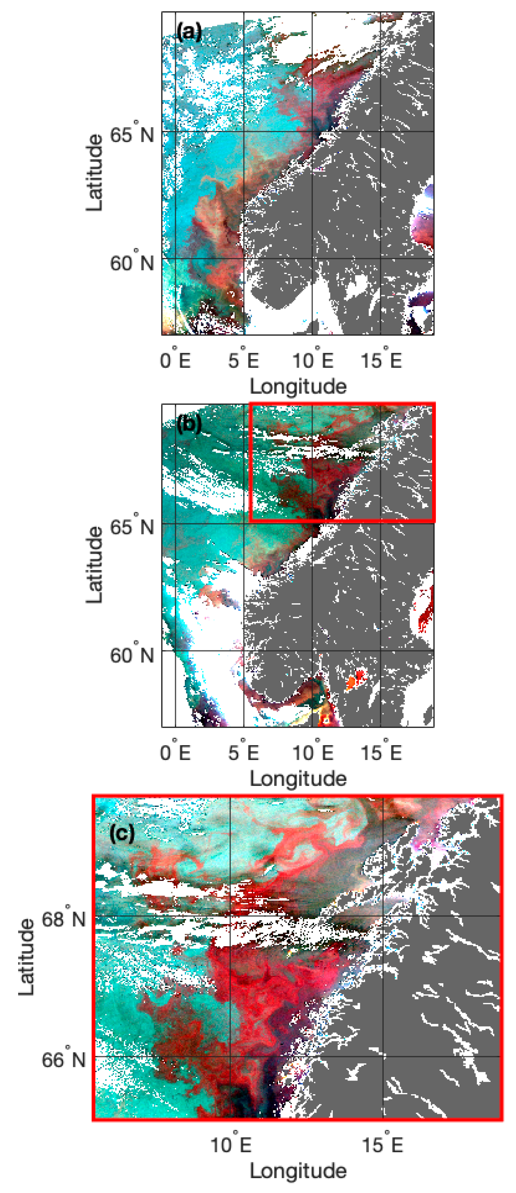
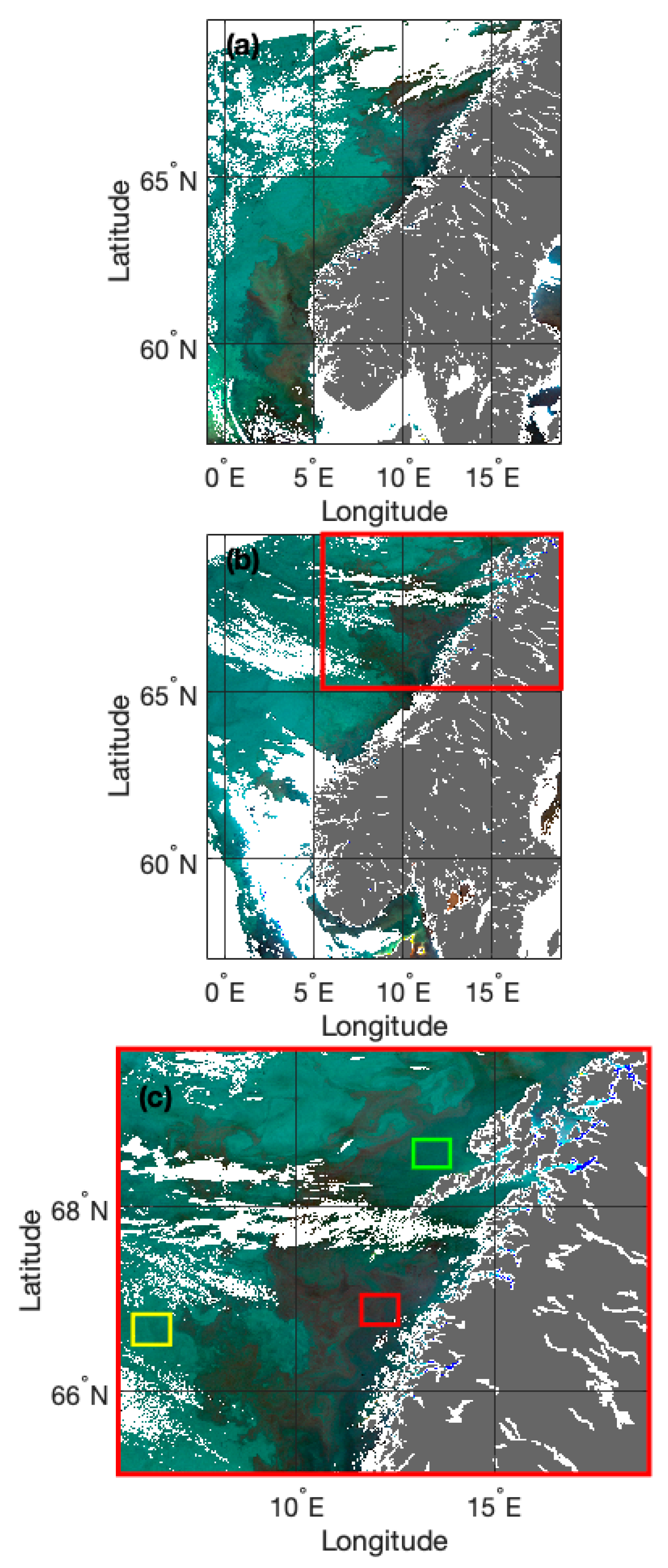
2.1. Study Site and Field Data

The Norwegian Sea is highly dynamic, with both the Norwegian Atlantic Slope Current (NwASC) and the Norwegian Coastal Current (NCC) dominating hydrodynamics in this region. In the shelf–slope area off the coast of northern Norway, large aggregations of C. finmarchicus are known to occur and are transported northward by both currents during the spring and summer [19]. Dong et al. [20] showed that the strong front between the NCC and the NwASC acts as a transport barrier in the region during the spring period when C. finmarchicus are ascending to the surface to feed. Thus, C. finmarchicus can be retained on the shelf for 30–70 days. In this study, we aim to resolve these well-established C. finmarchicus aggregations in the surface of the Northern Norwegian Sea through ocean colour remote sensing signals.

In situ data were collected during the Sea Patches cruise on the R/V Helmer Hanssen from 28 April until the 4 May 2017 off the coast of northern Norway. CDOM absorption, chlorophyll a concentration, phytoplankton abundance, vertical distribution, species identification and the pigment absorption of C. finmarchicus were measured at 8 stations within the study area. A full description of the methods used to collect each dataset, as well as the location of each station sampled, is given in Basedow et al. [17].

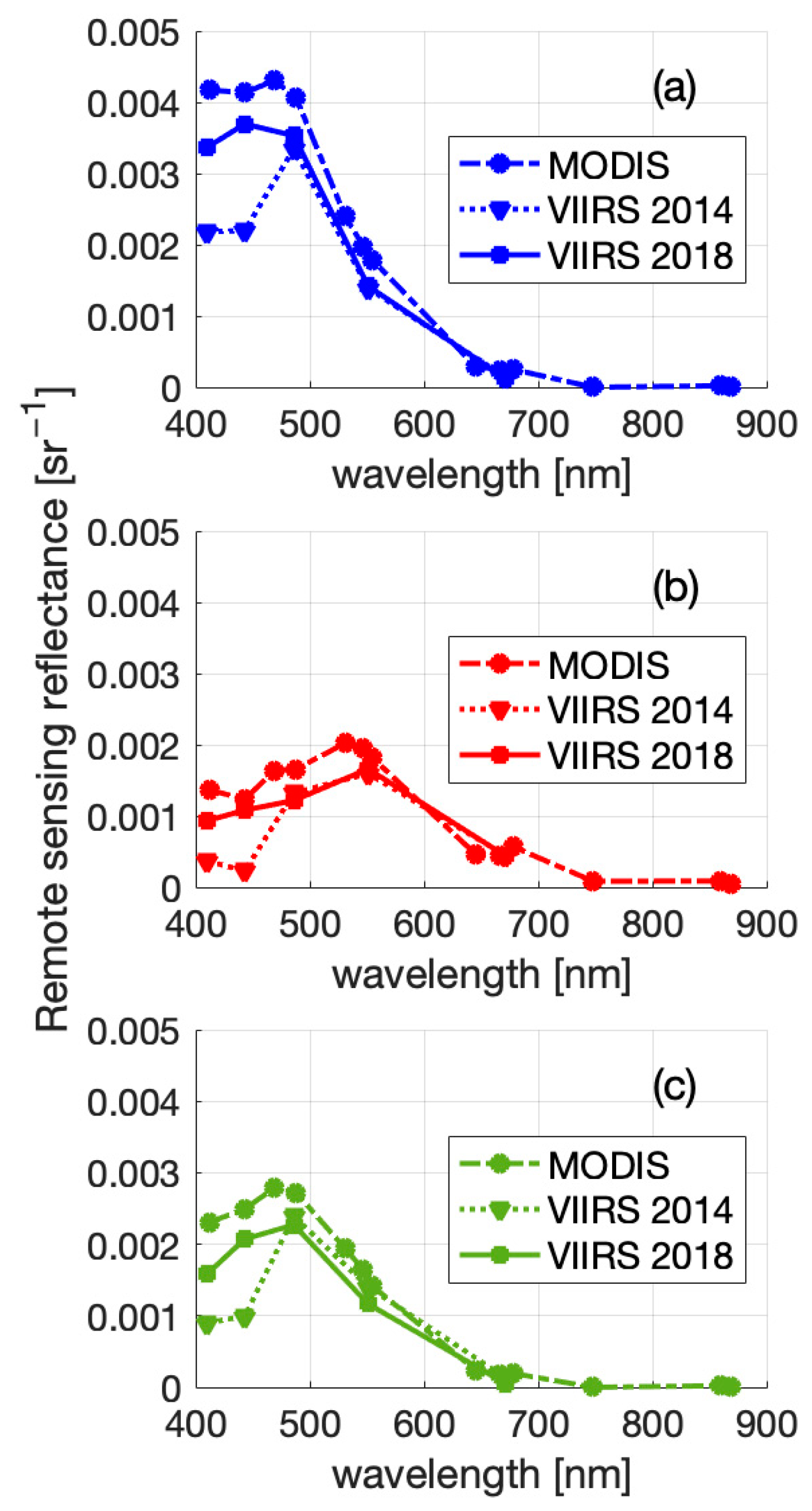
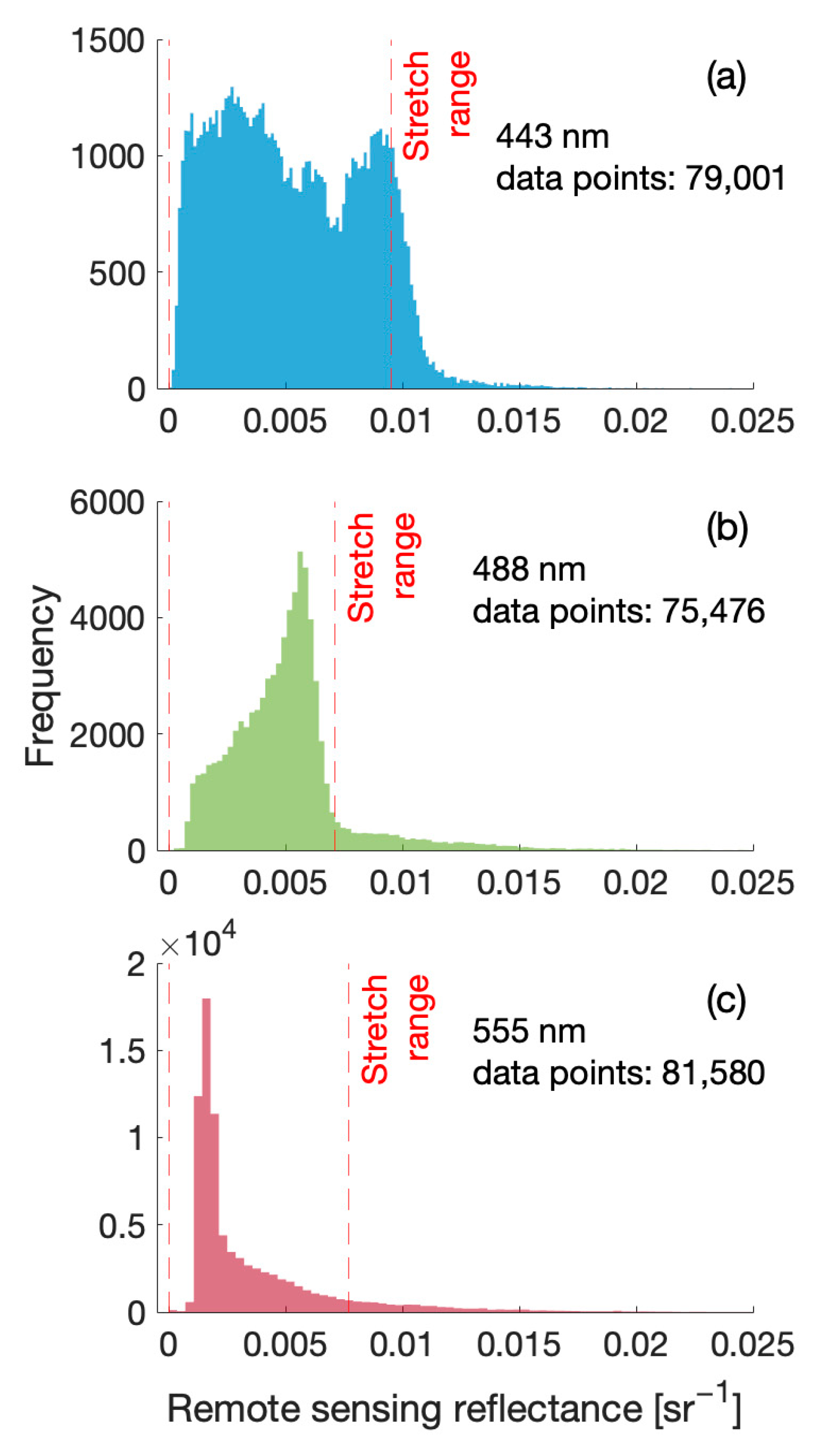
2.2. Satellite Data and eRGB Image Processing

The satellite data used in this study were from the MODIS Aqua sensor. MODIS was chosen instead of VIIRS as it has increased spectral resolution in the visible light region of the spectrum. Level 1A MODIS Aqua data were acquired from the National Aeronautics and Space Administration (NASA) Ocean Color archive (https://oceancolor.gsfc.nasa.gov/, accessed on 19 October 2020), with the R2018 calibration applied. MODIS Aqua has a 1 km resolution at its nadir. Between the cruise dates of 27 April and 4 May 2017, two relatively cloud-free scenes of the Norwegian Sea were obtained from the 28 and 29 April. These two scenes were downloaded and processed to level 2 using l2gen in the satellite data processing software package SeaDAS 7.5.1., with the standard atmospheric correction applied [21]. For this study, bands 412, 443, 469, 488, 531, 547, 555, 645, 667, 678 and 745 nm were processed. For each band, spectral remote sensing reflectance (R_rs) was downloaded. R_rs is calculated as follows:

$${\mathrm{R}}_{\mathrm{r}\mathrm{s}}=\frac{{\mathrm{L}}_{\mathrm{w}}}{{\mathrm{E}}_{\mathrm{d}}}$$

(1)

where L_w represents water-leaving radiance and E_d is downwelling radiance at the sea surface.

MODIS’ standard chlorophyll product ‘chlor_a’ was also processed. Chlorophyll estimations are calculated through the OCI algorithm, which combines a band difference approach for low chlorophyll concentrations [22] and a band ratio approach at higher chlorophyll concentrations [23]. Chlorophyll concentrations are first calculated using the three-band reflectance difference CI algorithm specified by Hu et al. [22]:

$${\mathrm{C}\mathrm{H}\mathrm{L}}_{\mathrm{C}\mathrm{I}}={10}^{({\mathrm{a}}_{0_{\mathrm{C}\mathrm{I}}}+{\mathrm{a}}_{1_{\mathrm{C}\mathrm{I}}}\times \mathrm{C}\mathrm{I})}$$

(2)

where the coefficients ${\mathrm{a}}_{0_{\mathrm{C}\mathrm{I}}}$ = −0.4287 and ${\mathrm{a}}_{1_{\mathrm{C}\mathrm{I}}}$ = 230.47, and CI is calculated as follows:

$$\mathrm{C}\mathrm{I}={\mathrm{R}}_{\mathrm{r}\mathrm{s}}555-\left[{\mathrm{R}}_{\mathrm{r}\mathrm{s}}443+\left(\frac{555-443}{667-443}\right)\times \left({\mathrm{R}}_{\mathrm{r}\mathrm{s}}667-{\mathrm{R}}_{\mathrm{r}\mathrm{s}}443\right)\right]$$

(3)

Chlorophyll is then calculated using the fourth-order polynomial ocean colour algorithm for the MODIS Aqua sensor (OC3M) [23]:

$${\mathrm{C}\mathrm{H}\mathrm{L}}_{\mathrm{O}\mathrm{C}3\mathrm{M}}={10}^{(\mathrm{a}+\mathrm{b}\mathrm{R}+\mathrm{C}{\mathrm{R}}^2+\mathrm{d}{\mathrm{R}}^5+\mathrm{e}{\mathrm{R}}^4)}$$

(4)

where R is calculated as follows:

$$\mathrm{R}={\mathrm{l}\mathrm{o}\mathrm{g}}_{10}\left\{\mathrm{m}\mathrm{a}\mathrm{x}\left[\left(\left.\frac{{\mathrm{R}}_{\mathrm{r}\mathrm{s}}433}{{\mathrm{R}}_{\mathrm{r}\mathrm{s}}547}\right),\left(\frac{{\mathrm{R}}_{\mathrm{r}\mathrm{s}}488}{{\mathrm{R}}_{\mathrm{r}\mathrm{s}}547}\right.\right)\right]\right\}$$

(5)

with a = 0.2424, b = −2.7423, c = 1.8017, d = 0.0015 and e = −1.228. For chlorophyll retrievals below 0.25 mg m⁻³ and above 0.35 mg m⁻³, the CI and the OC3M algorithms are used, respectively. For intermediate retrievals, when CI chlorophyll lies between these two values, the CI and OC3M algorithms is combined using a weighted approach where

$$\mathrm{C}\mathrm{H}\mathrm{L}=\frac{\mathrm{C}\mathrm{H}{\mathrm{L}}_{\mathrm{C}\mathrm{I}}({\mathrm{t}}_2-\mathrm{C}\mathrm{H}{\mathrm{L}}_{\mathrm{C}\mathrm{I}})}{{\mathrm{t}}_2-{\mathrm{t}}_1}+\frac{\mathrm{C}\mathrm{H}{\mathrm{L}}_{\mathrm{O}\mathrm{C}3\mathrm{M}}(\mathrm{C}\mathrm{H}{\mathrm{L}}_{\mathrm{C}\mathrm{I}}-{\mathrm{t}}_1)}{{\mathrm{t}}_2-{\mathrm{t}}_1}$$

(6)

where t₁ = 0.25 and t₂ = 0.35.

The data were then re-projected using the Mercator 1SP projection. Single-scene data were used as opposed to composites to maintain the temporal resolution in this highly dynamic region. Land and cloud masks were applied, as well as a mask to remove any pixels with negative values in the spectra, as this is an indication of atmospheric correction failure.

For each scene, eRGB images were generated in MATLAB (version R2022b) using three R_rs wavebands: 443 nm for the blue, 488 nm for the green and 555 nm for the red channel. A standard image processing procedure was implemented, where each band was stretched to include 95% of all pixels through the percentile stretching technique:

$${\mathrm{R}\mathrm{G}\mathrm{B}}^{\mathrm{o}\mathrm{u}\mathrm{t}}\left(\mathrm{\lambda }\right)=\mathrm{A}\left[\frac{{\mathrm{R}}_{\mathrm{r}\mathrm{s}}^{\mathrm{i}\mathrm{n}}\left(\mathrm{\lambda }\right)-{\mathrm{R}}_{\mathrm{r}\mathrm{s}}^{\mathrm{m}\mathrm{i}\mathrm{n}}\left(\mathrm{\lambda }\right)}{{\mathrm{R}}_{\mathrm{r}\mathrm{s}}^{\mathrm{m}\mathrm{a}\mathrm{x}}\left(\mathrm{\lambda }\right)-{\mathrm{R}}_{\mathrm{r}\mathrm{s}}^{\mathrm{m}\mathrm{i}\mathrm{n}}\left(\mathrm{\lambda }\right)}\right]$$

(7)

where at a given waveband, the R_rsⁱⁿ is the R_rs value of a pixel, and R_rs^min and R_rs^max represent the lower and upper stretch ranges. In this case, R_rs^min and R_rs^max are determined by the 2.5 and 97.5 percentiles of all pixels at each waveband. For these images, A = 1, as the RGB coordinates are scaled within the range 0–1. This calculation is conducted for each channel, producing a three-number RGB coordinate, representing the red, green and blue component of each pixel. Furthermore, a gamma correction of 0.7 was applied to the blue channel to improve contrast:

$${\mathrm{B}}_{\mathrm{o}\mathrm{u}\mathrm{t}}={\mathrm{A}{\mathrm{B}}_{\mathrm{i}\mathrm{n}}}^{\mathrm{\gamma }}$$

(8)

where, again, A = 1, B_in represents the calculated blue component of the RGB coordinate for each pixel and $\gamma$ represents the chosen gamma correction value (in this case 0.7).

2.3. Radiative Transfer Simulations

Above-surface spectral remote sensing reflectance (R_rs) was simulated using the Ecolight (version 5.2 Sequoia Scientific Inc., Bellevue, DC, USA) radiative transfer model. To produce a spectral look-up table, the model was populated with a range of log space constituent concentrations associated with the standard bio-optical model (CHL, MSS and CDOM). CHL was varied from 0.01 to 50 mg m⁻³, MSS from 0.01 to 25 g m⁻³ and CDOM from 0.01 to 0.5 m⁻¹ (CDOM concentrations are denoted by its absorption at 440 nm). This provided a total of 1008 runs, each with unique constituent concentration combinations. These ranges were used to broadly capture the natural optical variability in the ocean.

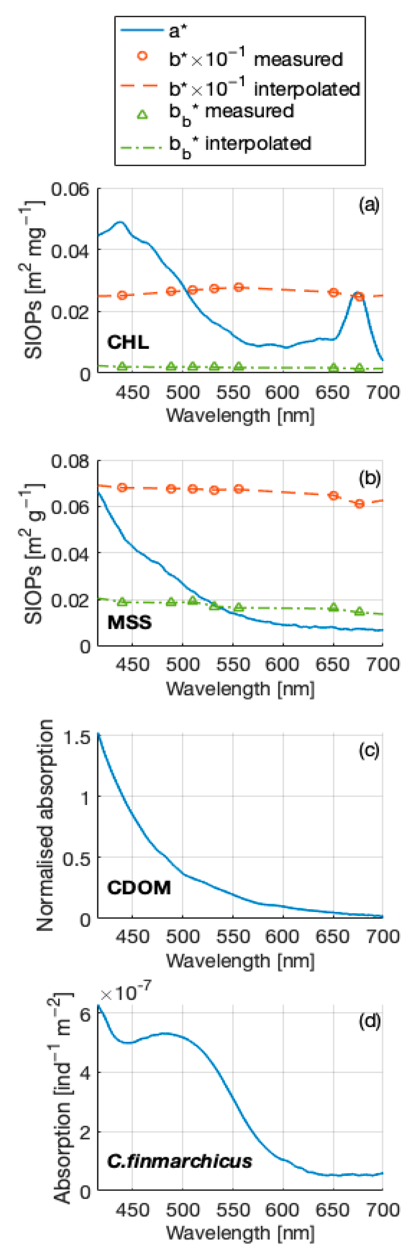
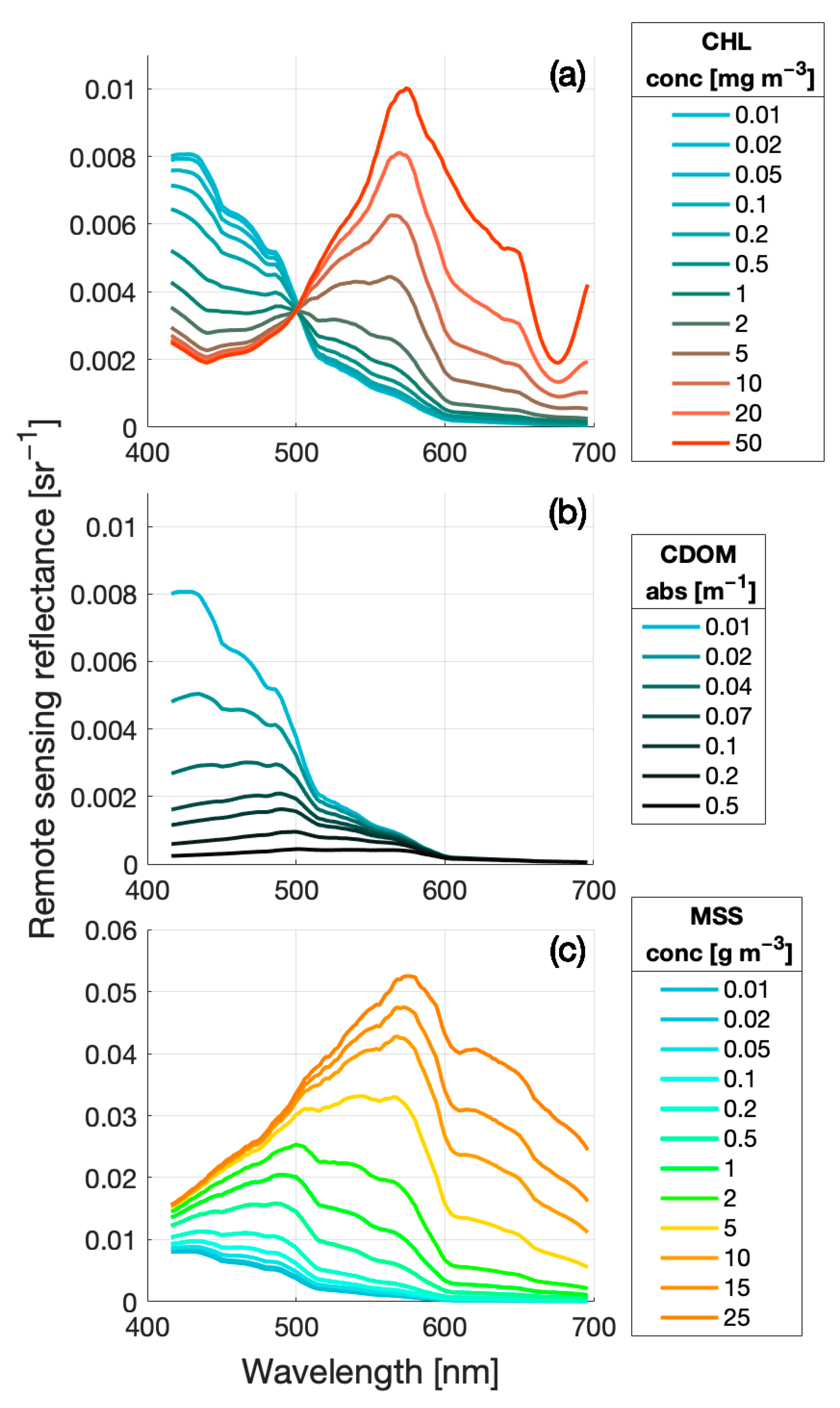
2.3.1. Bio-Optical Model Used

A bio-optical model is necessary to facilitate the simulation of water column IOPs from different optical constituent concentrations. In this study, a linear bio-optical model from the Ligurian Sea was used. All in situ data for the development of this bio-optical model were collected from the 13 to 29 March 2009 during a cruise campaign in the Ligurian Sea on board the NR/V Alliance. A full description of the sampling locations, data acquired, and methods used can be found in Bengil et al. [24], but they are summarised here. In situ non-water absorption (a_n) and attenuation (c_n) measurements were taken with a WETLabs 25 cm path length AC-9 instrument, operating at nine wavebands (10 nm FWHM) across the visible-NIR range (412, 440, 488, 510, 532, 555, 650, 676 and 715 nm). Corrections were applied for the temperature and salinity dependence of pure seawater using data from a Seabird SBE 19 plus CTD. Absorption measurements were corrected for scattering error using the proportional method [25]. In situ backscattering measurements (b_b) were made with a WETLabs BB-9 backscattering meter operating at nine wavebands centred on 412, 440, 488, 510, 595, 650, 676 and 715 nm. The data were corrected for path length absorption using the corrected AC-9 absorption data, and the backscattering of pure water was subtracted to obtain the particulate backscattering coefficient, as detailed by Lefering et al. [26]. BB-9 data were linearly interpolated to match AC-9 wavelengths.

The absorption of all dissolved and suspended components was measured using a point source integrating cavity absorption meter (PSICAM). Measurements of absorption by CDOM (a_CDOM) were made using a 1 m liquid waveguide capillary cell (LWCC) and an Ocean Optics USB2000 mini spectrometer. Total particulate absorption (a_p) was derived from subtracting a_CDOM from the PSICAM’s non-water absorption measurements. Total particulate absorption was also obtained through the filter pad method (Ferrari and Tassan, 1999) using a Shimadzu UV-2501 PC benchtop spectrophotometer. Absorption by phytoplankton (a_ph) was obtained through bleaching the samples to remove algal pigments, measuring the non-algal particulate absorption a_nap and subtracting this from a_p. PSICAM and LWCC data were utilised to determine path length amplification factors and scattering offset corrections through linear regression [26,27]. The filter pad corrections were applied to both bleached and unbleached absorption spectra.

CHL and total suspended solids (TSS) were measured in triplicate by colleagues from the Management Unit of the North Sea Mathematical Models (MUMM), with final values expressed as averages. Triplicate HPLC samples were analysed by the marine chemistry laboratory of the MUMM using a reversed phase, acetone-based method with a C18 column and a Jasco FP-1520 fluorescence detector. TSS concentration estimates were collected using pre-ashed, rinsed and pre-weighed 47 mm GF/F filters. Samples were carefully rinsed with ultrapure water to minimise salt retention. Filters were stored frozen and returned to the lab, where they were dried and re-weighed. TSS was numerically partitioned into biogenic (OSS) and mineral (MSS) components using the technique outlined in Bengil et al. [24]

The dataset collected during the Ligurian Sea cruise was from a total of 34 stations (after quality control), both onshore and offshore. The offshore stations consisted of deep, relatively clear waters, whereas the onshore stations were shallower and more turbid. Furthermore, onshore stations closer to the coast were influenced by fluvial sediments from the Arno River. As the offshore stations fit the criteria for case 1 waters, it was assumed that no MSS would be present at these stations and, thus, CHL-specific IOPs were derived from them. The CHL-specific IOPs were then used to further partition the onshore IOPs, which contained biogenic particulates (CHL) as well as MSS. This allowed for the determination of mineral-specific IOPs. CDOM was measured directly at each station.

The spectral material-specific IOPs (SIOPs) were determined via a linear regression forced through zero of the partitioned IOPs against the associated constituent concentrations from surface water samples, and this method is fully described by Lo Prejato et al. [28]. The SIOPs of each constituent used in this study are shown in Figure 2. The CHL component includes both the phytoplankton pigment absorption (a_ph) and biogenic detritus (a_det).

C. finmarchicus absorption was measured during the Sea Patches 2017 cruise in the Norwegian Sea and is presented in Basedow et al. [17] Here, live C. finmarchicus absorption was measured in triplicate in the PSICAM between 350 and 800 nm by means of a serial addition experiment. At each step of the experiment, seven to eight live copepods were sequentially added to seawater, using purified water as a reference. A simple linear regression between the number of individuals and absorption at each wavelength produced per-individual absorption spectra (Figure 2d). There is currently no suitable instrumentation that can provide estimates of large particle scattering or backscattering and so absorption is the only optical property used to represent C. finmarchicus in this study. Although scattering may have an unknown impact on the IOPs associated with C. finmarchicus, it is likely to be insignificant due to their large particle size, as theoretically demonstrated by Davies et al. [14].

2.3.2. Ecolight Radiative Transfer Modelling

Ecolight was populated with a range of constituent concentrations in the surface layer (0 m depth), with a homogenous water column and infinite depth set up. Ecolight was provided with latitude and longitude coordinates of the study area, as well as the time and date the satellite data were collected, in order to calculate the solar zenith angle. The model was set up with zero cloud cover, a windspeed of 7.9 m s⁻¹, a refractive index of 1.34, water temperature of 5.5 °C and a salinity of 34 psu. Note that the surface reflectance presented here does not include sun glint effects. Simulations were conducted between 412 and 714 nm at 2 nm intervals. Input files containing the IOPs generated from varying constituent concentrations and the bio-optical model described above were generated using a bespoke MATLAB script. The partitioned IOPs from the Ligurian Sea were added together to produce total absorption (a_tot) attenuation (c) and backscattering (b_{b tot}) spectra. These were then presented to Ecolight in the form of synthesised AC and BB instrument files. Raman scattering was the only form of inelastic scattering included the model, as CHL and CDOM fluorescence were not included.

2.4. Quantification of Percieved Colour Difference

In order to quantify perceived difference in eRGB colour coordinates, the International Commission on Illumination (CIE) Delta E 2000 (ΔE₂₀₀₀) algorithm was utilised. This algorithm quantifies the visual similarity between two different coordinates in the L*a*b colour space, with higher ΔE₂₀₀₀ values signalling more visually different colours. The first ΔE colour difference algorithm developed was ΔE₁₉₇₆, which provided a difference value derived from the Euclidian distance between two coordinates in the L*a*b colour space. However, this does not take into account the perceptual non-uniformity of the human eye response to colour, especially with highly saturated colour values. Thus, the newer iterations of the algorithm include weighting factors for lightness, chroma and hue value, which are all important when considering visual perception. The ΔE₂₀₀₀ algorithm is the most sophisticated and accurate adaptation of ΔE to date, providing significant improvements to the lightness calculation and enhancing performance for the blue and grey colours [29]. This is of potential importance for images of clear blue case 1 waters.

The MATLAB function ‘imcolordiff’ from the image processing toolbox was used to implement this algorithm. This function first converts RGB colour coordinates to their associated L*a*b coordinates using the function ‘rgb2lab’. The ΔE₂₀₀₀ algorithm is then applied to the coordinates, following the formulae described in the implementation document by Sharma et al. [30]. The output is a ΔE₂₀₀₀ value from 0 to 100, with 0 being no visual difference between the two input colours and 100 signifying colours that are opposites on the colour wheel. Colour difference thresholds can vary according to application; however, the printing industry’s ΔE₂₀₀₀ threshold of 4 can be used as a guideline [31]. Therefore, colour comparisons that yield ΔE₂₀₀₀ values below 4 can be considered visually insignificant to the untrained eye.

3. Results

3.1. Standardised eRGB Imagery

The images produced from the stretching method of excluding 5% of pixels in each band are visually inconsistent (Figure 3). Despite being only one day apart, the colour of the offshore water varies significantly, as do the red pixels that appear along the coast. Furthermore, when the image is cropped to enlarge the suspected patch of C. finmarchicus (Figure 3c) and the same stretching method is applied, the colour of the sub-scene varies significantly. This is because the range applied to each of the bands is dependent on the information within the image (or cropped image) itself. This makes it difficult to distinguish variance caused by the optical properties of the water column from that caused by the processing method applied.

To overcome this issue, a standardised stretch range was developed using an in situ dataset of global R_rs values compiled by Valente et al. [32]. All measurements ± 5 nm of each waveband were included to ensure there were enough data points (Figure 4). The minimum of the range was set to 0 and the maximum was determined by the 90th percentile of each band. This provided the best visual results for the Norwegian Sea images. In addition, a gamma correction of 0.8 applied in MATLAB to the blue band was determined to provide optimal visual contrast (Equation (8)). Once the ranges were applied to the images using Equation (7) and processed, the visual inconsistency between the images was removed (Figure 5). From the processed sub-scene of the red patch, three regions of interest (ROIs) were identified for analysis. These three regions represent inside the suspected patch of C. finmarchicus, as well as an offshore region and a coastal area (Figure 5c).

3.2. eRGB Colour Simulation

The R_rs spectra simulated from the 1008 different constituent concentration combinations were converted into their associated standardised eRGB coordinates. To achieve this, simulated R_rs values at wavelengths 442 nm, 488 nm and 554 nm (following the MODIS eRGB image processing method described above) were extracted and converted to eRGB coordinates using Equation (7), with the standardised range applied. A gamma correction of 0.8 was also applied to the blue channel as per Equation (8). Some of the RGB coordinates derived from the simulated spectra exceeded the standard 0–1 range of the RGB colour space. This is because the highest constituent concentrations simulated are likely not represented by the 0–90th percentile range of the in situ dataset. For these coordinates, minimum–maximum normalisation was applied.

From this, a look-up table (LUT) of eRGB colours associated with the standard bio-optical model was generated. Figure 6 shows the impact of varying each of these constituents in isolation on both the spectra and the associated eRGB colour value. It is evident from Figure 6a that high chlorophyll concentrations alone (>10 mg m⁻³) produce red hues in this colour space through reduced blue reflectance and increased green/red reflectance. Furthermore, the addition of high concentrations of MSS (>5 g m⁻³) increases reflectance across the spectrum, especially in the green/red, and produces orange hues (Figure 6c). Conversely, CDOM acts to suppress reflectance across the spectrum, resulting in dark, brown/black hues at high concentrations (Figure 6b). CDOM acts differently to the other two standard constituents as it is dissolved and, therefore, does not scatter light.

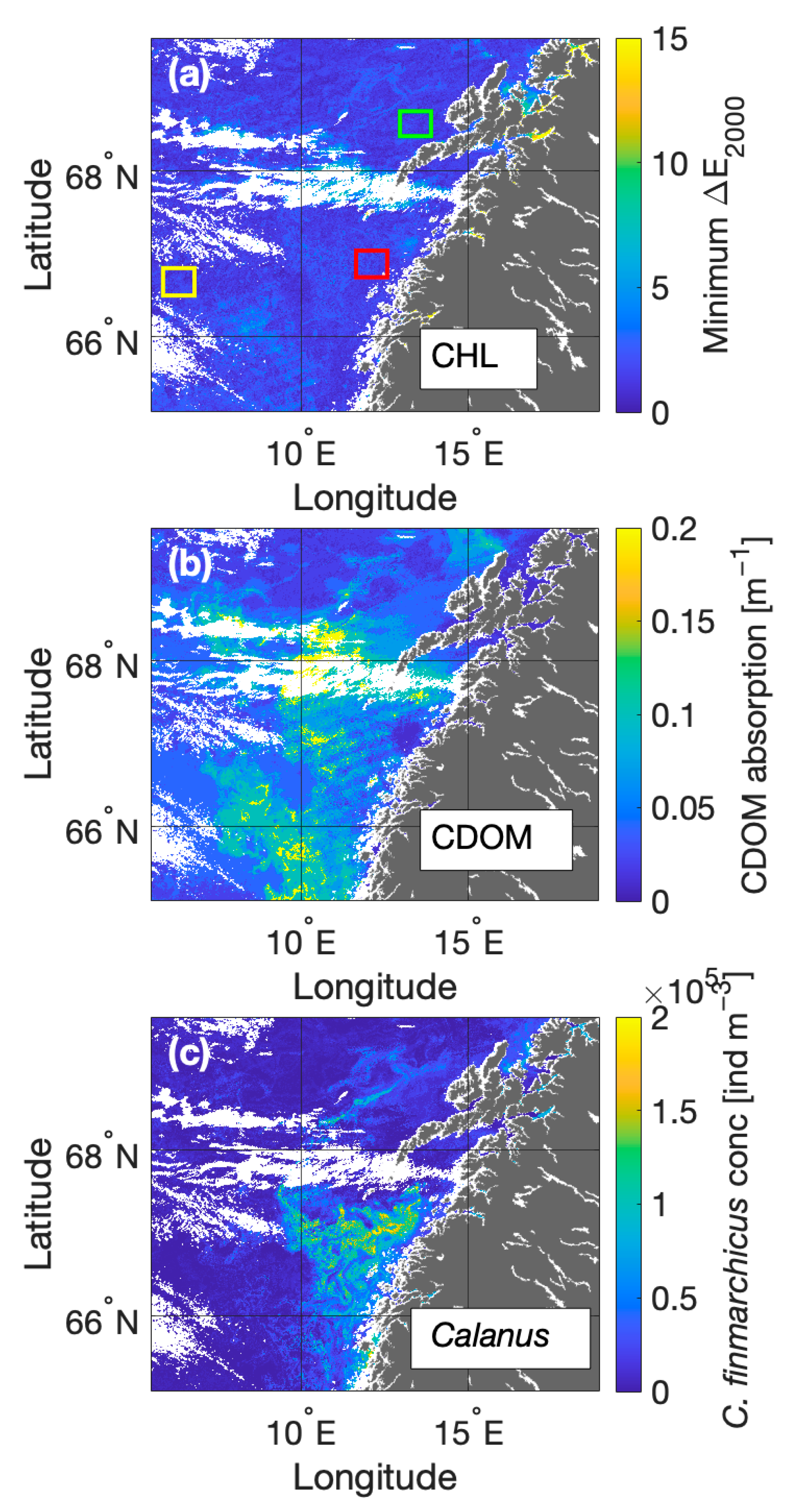
3.3. Anomaly Detection

Each pixel in the sub-scene image was compared to the eRGB coordinate LUT (a total of 1008 eRGB coordinates) using the ΔE₂₀₀₀ colour difference algorithm described in Section 2.4. This allowed for the identification of regions where the optics of the water column are not well described by the standard bio-optical model. For every pixel, the minimum ΔE₂₀₀₀ value was extracted and mapped, producing an anomaly map where regions not well described by the standard bio-optical model are highlighted by relatively large minimum ΔE₂₀₀₀ values (Figure 7). It is clear that the coastal and offshore ROIs have a low minimum ΔE₂₀₀₀ relative to inside the red patch, suggesting that the red patch is not well described by the standard bio-optical model alone.

The concentrations of each constituent required to produce the best ΔE₂₀₀₀ colour matches were extracted and mapped (Figure 8). ΔE₂₀₀₀ estimated chlorophyll concentrations reached a high of 2 mg m⁻³ within the red patch (Figure 8a). CDOM concentrations were unexpectedly high, at 0.2 m⁻¹ (absorption at 440 nm) in and around the patch (Figure 8b). As in situ measurements of CDOM during the 2017 Sea Patches cruise reached a maximum of 0.06 m⁻¹, these estimates are most likely erroneous. Finally, MSS remained uniform throughout the region, with a median value of 0.03 g m⁻³ (Figure 8c).

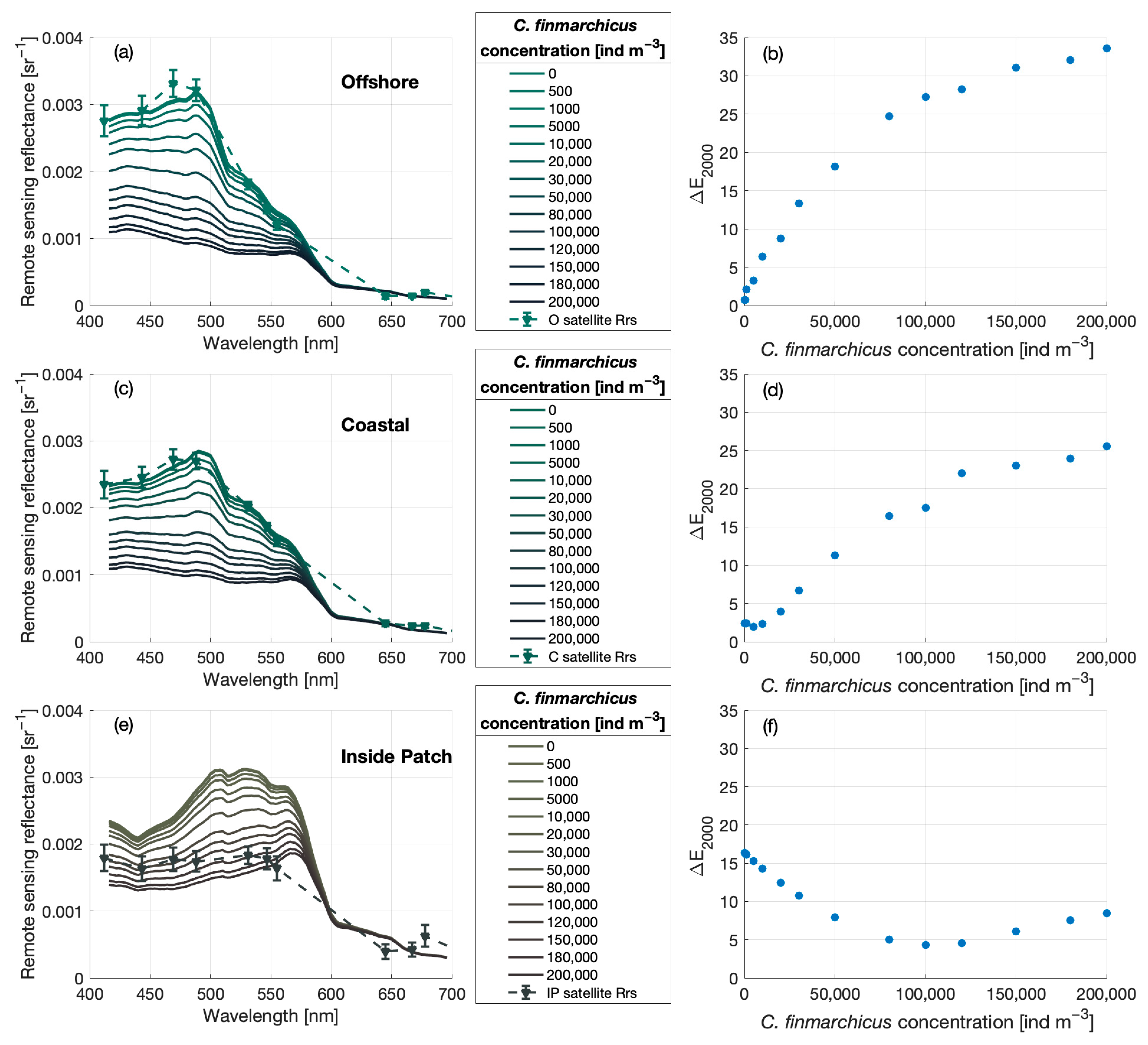
3.4. Impact of C. finmarchicus Absorption on Reflectance Signals

The impact of C. finmarchicus on satellite reflectance signals was simulated in Ecolight and compared to the median satellite reflectance spectra of the three identified ROIs (Figure 9). Median spectra were used to represent the ROIs instead of individual pixel spectra to reduce the potential error associated with the high degree of variability in this region. For the initial spectra without the presence of C. finmarchicus, an MSS value of 0.03 g m⁻³ was used for all ROIs, along with the median chlorophyll estimate derived from the satellite data (0.3 mg m⁻³, 0.6 mg m⁻³, and 2 mg⁻³ for offshore, coastal, and inside patch ROIs, respectively). The CDOM input for the coastal and inside patch areas was set to 0.05 m⁻¹, as this was the median value obtained from in situ measurements in 2017. A CDOM value of 0.04 m⁻¹ was used for the offshore ROI to provide the best spectral match with the median satellite spectra.

Overall, C. finmarchicus absorption acts to reduce R_rs across the blue/green part of the spectrum (from 412 to around 580 nm). This effect is similar to that of CDOM (Figure 6b). The results also indicate that for the offshore and coastal ROIs, the spectral match is worsened and ΔE₂₀₀₀ values increase with the addition of C. finmarchicus (Figure 9a–d). Conversely, for the inside patch ROI, both the spectral shape and magnitude were improved with the addition of C. finmarchicus, and ΔE₂₀₀₀ analysis indicated that 100,000 individuals m⁻³ provided the best colour match in this region (Figure 9e,f).

Estimating Surface C. finmarchicus Concentrations from eRGB Imagery

To provide an estimate of patch extent and surface concentrations, Calanus finmarchicus were added as a varying constituent to the model. To facilitate this, MSS concentrations were set to 0.03 g m⁻³, as MSS appears to remain low and relatively stable in this region (Figure 8c). As a result, a new RGB LUT with a total of 1176 unique constituent concentration combinations was created. The new anomaly map shows a much lower minimum ΔE₂₀₀₀ across the entire image, especially for the inside patch ROI (Figure 10a). Furthermore, anomaly remains low in the coastal and offshore ROIs. Thus, the lack of C. finmarchicus absorption in the original model potentially accounts for a large amount of the anomaly present in the image, especially within the red patch. Although still high, estimated concentrations of CDOM have been significantly reduced with the addition of C. finmarchicus absorption (Figure 10b). Notably, within the red patch where CDOM concentrations have significantly reduced, concentrations of C. finmarchicus appear to be high (Figure 10c). Surface concentration estimates of the copepod in this patch range from 80 to 150,000 individuals m⁻³, with maximum values reaching 200,000 individuals m⁻³.

3.5. Impact of C. finmarchicus Absorption on OC3M Algorithm Performance

When the colour matching technique is applied with C. finmarchicus included, the ΔE₂₀₀₀ CHL increased compared to that produced by the standard bio-optical model (Figure 8a). However, estimates are generally lower than the standard MODIS ‘chlor_a’ product generated using the OCI algorithm (Figure 11). For the inside patch ROI, the median CHL value predicted from the ΔE₂₀₀₀ method is 1 mg m⁻³, whereas the satellite CHL product predicts a median value of 2 mg m⁻³. Furthermore, OCI predicts maximum values of 5 mg m⁻³ within the red patch, whereas these maximum values are much less frequently reached using the ΔE₂₀₀₀ approach.

In order to investigate the impact of C. finmarchicus absorption on MODIS’ chlorophyll retrievals, simulated spectra from each ROI with increasing C. finmarchicus concentrations were put through OC3M (Equations (4) and (5)). The impact of C. finmarchicus on OC3M specifically was tested as these copepods graze on phytoplankton and are, therefore, likely to be found at the surface when concentrations of chlorophyll are greater than 0.35 mg m⁻³ (for example, during the spring bloom) [3,33].

The results indicate that across all three ROIs, increasing C. finmarchicus concentrations lead to an increase in chlorophyll estimates, despite the modelled CHL remaining constant during the simulations (Figure 12). Estimates of CHL in the coastal and offshore ROIs more than doubled with the addition of 200,000 individuals m⁻³. Within the patch ROI, estimates increased by 1 mg m⁻³. This explains the lower CHL values predicted through the ΔE₂₀₀₀ method relative to the standard satellite CHL product, and indicates that surface aggregations of C. finmarchicus would lead to an overestimation of CHL in water bodies with varying optical properties.

4. Discussion

Satellite-derived RGB imagery is routinely used to identify environmental phenomena and observe changes in the state of marine ecosystems over large spatio-temporal scales. Enhanced RGB (eRGB) imagery can be a useful tool when looking at the ocean, as it increases the contrast of optical constituents in the water by using a green waveband (555 nm in this study) as the ‘red’ component in the image. However, these images can be processed in a variety of ways. One method of applying contrast stretching to RGB imagery that is widely used is to exclude 5% of pixels in each band (the percentile stretching technique). This method relies upon the information contained within the image to calculate the band ranges and, thus, produces visually inconsistent imagery that proves to be of limited use when attempting to identify features over multiple images. In this study, a contrast stretch range for each band was developed using a global dataset of in situ R_rs values [34], which provided visual consistency between the images processed. By applying the same stretch range, variance due to the processing method is removed and more quantitative information can be gained from the eRGB imagery.

Whilst the dataset used to determine the ranges in this study nominally had global coverage, it is likely that these ranges may need to be further adapted for other areas. The range in this study was selected to provide the best visual output for the Norwegian Sea region, and for this, the upper 90th percentile was set as the limit. In clear blue waters, for example, it is likely that the 443 nm and 488 nm wavebands would have high reflectance relative to the Norwegian Sea and would exceed the ranges applied in this study. Furthermore, a lower limit of 0 is likely to be too low for satisfactory visual representation in case 1 waters, where blue reflectance is unlikely to fall to these values. Therefore, whilst this range can be applied to case 2 waters, it may need to be altered when applying the general method to optically clear, case 1 waters.

Once a meaningful eRGB colour space was established, it became possible to develop an eRGB LUT from the R_rs spectra of the 1008 unique constituent combinations simulated in Ecolight. From the results presented, it is clear that ‘red’ hues can be produced in this colour space with the addition of large chlorophyll concentrations alone. This is likely because the ‘red’ band in these images is actually a green waveband (555 nm). As a result, large phytoplankton blooms may produce red pixels in images such as the ones in this study. However, when the RGB coordinates of the image were numerically compared with the standard bio-optical model eRGB LUT, the potential patch of C. finmarchicus was flagged as an optically anomalous feature. This suggests that the red patch is not well described by the standard bio-optical model alone.

In situ measurements suggest that C. finmarchicus was present in relatively high concentrations in the surface waters during the time period in which these images were taken [17]. Analysis of the IOPs of the water column, along with the phytoplankton assemblage, indicates that there was no other material present excluded by the standard bio-optical model (e.g., dinoflagellates) that would result in a red signal similar to C. finmarchicus. Therefore, C. finmarchicus absorption was introduced into the model to address the anomaly. The addition of C. finmarchicus absorption leads to optical closure between the modelled and median satellite spectra within the red patch ROI. The lowest ΔE₂₀₀₀, i.e., the best visual matchup, is achieved with the addition of 100,000 individuals m⁻³. The opposite is true in the coastal and offshore ROIs, where the addition of C. finmarchicus leads to an increasing mismatch between the modelled and satellite derived spectra. Furthermore, the anomalous feature evident in the initial minimum ΔE₂₀₀₀ map is significantly reduced with the addition of C. finmarchicus absorption. This strongly suggests that the red patch previously identified by Basedow et al. [17] was influenced to a significant degree by a C. finmarchicus aggregation. It is likely that both phytoplankton and C. finmarchicus are influencing the water column optics within the feature, as C. finmarchicus are known to emerge at the surface after overwintering to feed on phytoplankton during the spring bloom at this time of year [3,33,35].

The C. finmarchicus concentration maps indicate surface concentrations of between 80,000 and 200,000 individuals m⁻³ within the extent of the red patch. These concentrations are an order of magnitude greater than those measured in the 2017 Sea Patches cruise, during which the maximum reached was 16,000 individuals m⁻³ at the surface. There are two potential reasons for this apparent mismatch. Firstly, the zooplankton abundance estimates during the 2017 Sea Patches cruise were derived from Multinet samples, which sample the surface 5 m of the water column. Abundances are calculated over the surface 5 m, but it is not possible to tell where in the water column these organisms were distributed. If they were concentrated in the surface metre, for example, the surface abundances would be 80,000 individuals m⁻³, which correlates more closely with the concentration maps derived from satellite data.

Another possible reason for the mismatch between satellite concentration estimates and in situ samples is animal evasion. Traditional zooplankton sampling techniques (i.e., net sampling or trawls) are invasive and likely disturb the community that they are attempting to sample. Unlike phytoplankton, C. finmarchicus have the ability to swim, and as, a result, may evade capture. A recent study conducted on fish and zooplankton populations in the Arctic during polar night found that a normal working light from a ship could disrupt populations down to 200 m depth and up to 0.125 km² around the ship [36]. Although data collected during the polar night are not directly transferable to the northern Norwegian Sea in spring (ca. 20 h daylight end of April), this study highlights the sensitivity of these organisms to disturbances. Therefore, the possibility that ship engine noise and disturbance from net sampling will also result in animal evasion must be considered. In fact, a recent study by Bandara et al. [37] conducted in the Norwegian Sea found concentrations of up to 165,000 individuals m⁻³ of C. finmarchicus at 10 m depth. This study collected high-frequency acoustic data in 2018 by means of a silent autonomous surface glider (Sailbuoy). This far less invasive method of data collection is likely to cause much lower disturbance to animal behaviour and, therefore, has the potential to return more accurate results. Taken together, all of these results point to a potential problem with the underestimation of population densities for these mobile copepods using traditional shipboard sampling techniques, which could have significant implications for both management strategies and ecological modelling.

It is important to note that satellite data only have the ability to resolve surface populations of C. finmarchicus, and no information on populations at significant depths can be retrieved. The optical depth is primarily determined by the constituents in the water column and is typically between 5 and 10 m. Whilst we cannot resolve populations at depth, these results are useful for providing a non-invasive method to identify and quantify surface populations, as well as track the spatio-temporal variation of these large-scale features. Additionally, the optical characterisation of C. finmarchicus in this study is limited to absorption alone, as no data are currently available on backscattering effects. Whilst Davies et al. [14] theoretically demonstrated that the impact of larger millimetre-sized particles on backscattering is likely to be very low, they may still impact satellite reflectance signals to an unknown degree. Thus, future work is required to better understand the optical properties of these organisms.

The MODIS chlorophyll product provided chlorophyll estimates that were generally higher than those of the ΔE₂₀₀₀ method. When the impact of C. finmarchicus on the OC3M algorithm was analysed, the results indicated that the inclusion of C. finmarchicus absorption leads to an overestimation of chlorophyll concentrations across all three ROIs. C. finmarchicus absorbs strongly in the blue part of the spectrum and peaks at around 480 nm (Figure 2d). As the OC3M algorithm relies on the ratio of the blue (443 nm or 488 nm band depending on water type) to green (547 nm) bands to estimate chlorophyll (Equations (2) and (3)), greater reflectance in the green relative to the blue will lead to an overestimation in chlorophyll concentrations. This is important to consider in regions where surface C. finmarchicus populations are significant.

The use of eRGB coordinates and minimum ΔE₂₀₀₀ as a method of anomaly detection allows for greater understanding of how these features present in RGB imagery. In the case of C. finmarchicus specifically, eRGB coordinates resolve the impact of these organisms well, as the 488 nm waveband is used, which corresponds with their absorption peak of 480 nm. In a wider context, this method can be generally applied to identify regions or features that deviate from the standard bio-optical model. This could be a valuable tool to support targeted sampling efforts for optically complex regions.

Something to consider when applying this method for the identification of zooplankton aggregations is the similarity in spectral signature between CDOM and C. finmarchicus absorption. Although their spectral shape is different, both have broadly the same effect of reducing reflectance in the blue/green part of the spectrum. Anomaly within the red patch was evident from the initial comparison with the standard bio-optical model LUT (Figure 7). However, the erroneously high CDOM estimates within the patch suggest that not all of the optical signature associated with C. finmarchicus has been flagged as anomalous using this method. In this study, the addition of C. finmarchicus absorption, especially within the identified patch, significantly improved the CDOM concentration estimates (Figure 10). This highlights the importance of looking at not just the anomaly maps, but also the constituent concentrations providing the best match up. Furthermore, knowledge of the typical concentrations of CDOM within the region of study is useful. In this case, in situ measurements of CDOM made during the Sea Patches cruise allowed for the identification of erroneously high estimates. Although it is clear that this method has the ability to discern somewhat between CDOM and C. finmarchicus, it is possible that there is still a degree of underestimation of C. finmarchicus populations due to limited ability to distinguish their optical signal from that of CDOM using only three wavebands.

A potential solution to this problem is a full spectral matching approach of the current multispectral data available, extendable in the future to hyperspectral data. The use of all the spectral information available may aid in resolving finer-scale optical features such as this, and will form the subject of further work in this area. With the advent of NASA’s PACE mission, global satellite-derived hyperspectral data will become accessible. Better resolution of surface zooplankton swarm formations and concentrations may benefit from the new capabilities that PACE will offer.

5. Conclusions

This study demonstrated, through the use of a novel eRGB colour matching technique, the ability to identify and characterize dense surface aggregations of the zooplankton species Calanus finmarchicus from satellite-derived ocean colour imagery. Concentration estimates of the patch in the northern Norwegian Sea were an order of magnitude greater than those measured in situ during the time period and point to a potential animal evasion issue, due to the invasive nature of traditional ship-based sampling techniques. This could lead to significant population underestimations and, therefore, more work is required to both characterize potential evasion behaviour and develop less invasive sampling methods that will reduce population disturbance for ground truthing. Furthermore, this study demonstrated that C. finmarchicus absorption can lead to an overestimation of chlorophyll and CDOM retrievals, which should be considered in regions where these organisms are present in surface waters. The methodology described in this study is derived from a global in situ dataset and, therefore, there is scope for this method to be used to detect optical anomaly elsewhere. However, more work on the adaptability of this method for clear blue case 1 waters is required, where the blue signal is much larger than in this study region. In any case, it is clear that larger particles, such as zooplankton, can influence ocean colour signals and need to be taken into consideration when characterizing the optical properties of oceanic environments.

References

1. Tilstone, G.H.; Pardo, S.; Dall’Olmo, G.; Brewin, R.J.W.; Nencioli, F.; Dessailly, D.; Kwiatkowska, E.; Casal, T.; Donlon, C. Performance of Ocean Colour Chlorophyll a algorithms for Sentinel-3 OLCI, MODIS-Aqua and Suomi-VIIRS in open-ocean waters of the Atlantic. Remote Sens. Environ. 2021, 260, 112444. [Google Scholar] [CrossRef]
2. Blondeau-Patissier, D.; Gower, J.F.R.; Dekker, A.G.; Phinn, S.R.; Brando, V.E. A review of ocean color remote sensing methods and statistical techniques for the detection, mapping and analysis of phytoplankton blooms in coastal and open oceans. Prog. Oceanogr. 2014, 123, 123–144. [Google Scholar] [CrossRef] [Green Version]
3. Falk-Petersen, S.; Mayzaud, P.; Kattner, G.; Sargent, J.R. Lipids and life strategy of Arctic Calanus. Mar. Biol. Res. 2009, 5, 18–39. [Google Scholar] [CrossRef] [Green Version]
4. Melle, W.; Runge, J.; Head, E.; Plourde, S.; Castellani, C.; Licandro, P.; Pierson, J.; Jonasdottir, S.; Johnson, C.; Broms, C.; et al. The North Atlantic Ocean as habitat for Calanus finmarchicus: Environmental factors and life history traits. Prog. Oceanogr. 2014, 129, 244–284. [Google Scholar] [CrossRef] [Green Version]
5. Wiborg, K.F. Fishery and commercial exploitation of Calanus finmarchicus in Norway. ICES J. Mar. Sci. 1976, 36, 251–258. Available online: https://academic.oup.com/icesjms/article/36/3/251/639243 (accessed on 8 March 2023).
6. Eilertsen, K.-E.; Mæhre, H.K.; Jensen, I.J.; Devold, H.; Olsen, J.O.; Lie, R.K.; Brox, J.; Berg, V.; Elvevoll, E.O.; Østerud, B. A Wax Ester and Astaxanthin-Rich Extract from the Marine Copepod Calanus finmarchicus Attenuates Atherogenesis in Female Apolipoprotein EDeficient Mice. J. Nutr. 2012, 142, 508–512. [Google Scholar] [CrossRef] [Green Version]
7. Pedersen, A.M.; Vang, B.; Olsen, R.L. Oil from Calanus finmarchicus—Composition and Possible Use: A Review. J. Aquat. Food Prod. Technol. 2014, 23, 633–646. [Google Scholar] [CrossRef]
8. Vilgrain, L.; Maps, F.; Trudnowska, E.; Basedow, S.L.; Madoui, A.; Niehoff, B.; Irisson, J.-O.; Ayata, S.-D. Copepods’ true colours: Pigmentation as an indicator of fitness. Ecosphere 2023. [Google Scholar] [CrossRef]
9. Yiki, V. Biological functions and activities of animal carotenoids. Pure Appl. Chem. 1991, 63, 141–146. [Google Scholar] [CrossRef]
10. Morel, A.; Prieur, L. Analysis of variations in ocean color. Limnol. Oceanogr. 1977, 22, 709–722. [Google Scholar] [CrossRef]
11. Stramski, D.; Kiefer, D.A. Light scattering by microorganisms in the open ocean. Prog. Oceanogr. 1991, 28, 343–383. [Google Scholar] [CrossRef]
12. Stramski, D.; Mobley, C.D. Effects of microbial particles on oceanic optics: A database of single-particle optical properties. Limnol. Oceanogr. 1997, 42, 538–549. [Google Scholar] [CrossRef] [Green Version]
13. Mobley, C.D. Optical Properties of Water. In Light and Water: Radiative Transfer in Natural Waters; Mobley, C.D., Preisendorfer, R.W., Eds.; Academic Press: Cambridge, UK, 1994. [Google Scholar]
14. Davies, E.J.; Basedow, S.L.; McKee, D. The hidden influence of large particles on ocean colour. Sci. Rep. 2021, 11, 3999. [Google Scholar] [CrossRef] [PubMed]
15. Bullen, G. Makerel and Calanus. Nature 1913, 91, 531. [Google Scholar] [CrossRef]
16. Sars, G.O. An Account of the Crustacea of Norway: Copepoda, Calanoida; University Museum of Bergen: Bergen, Norway, 1903; Volume 4. [Google Scholar]
17. Basedow, S.L.; McKee, D.; Lefering, I.; Gislason, A.; Daase, M.; Trudnowska, E.; Egeland, E.S.; Choquet, M.; Falk-Petersen, S. Remote sensing of zooplankton swarms. Sci. Rep. 2019, 9, 686. [Google Scholar] [CrossRef] [Green Version]
18. Weng, F.; Choi, T.; Cao, C.; Zhang, B. Reprocessing of SUOMI NPP VIIRS sensor data records and impacts on environmental applications. In Proceedings of the 2017 IEEE International Geoscience and Remote Sensing Symposium (IGARSS), Fort Worth, TX, USA, 23–28 July 2017; pp. 293–296. [Google Scholar] [CrossRef]
19. Zhu, Y.; Tande, K.S.; Zhou, M. Mesoscale physical processes and zooplankton transport-retention in the northern Norwegian shelf region. Deep. Sea Res. Part II Top. Stud. Oceanogr. 2009, 56, 1922–1933. [Google Scholar] [CrossRef]
20. Dong, H.; Zhou, M.; Hu, Z.; Zhang, Z.; Zhong, Y.; Basedow, S.L.; Smith, W.O., Jr. Transport Barriers and the Retention of Calanus finmarchicus on the Lofoten Shelf in Early Spring. J. Geophys. Res. Oceans 2021, 126, e2021JC017408. [Google Scholar] [CrossRef]
21. Mobley, C.D.; Werdell, J.; Franz, B.; Ahmad, Z.; Bailey, S. Atmospheric Correction for Satellite Ocean Color Radiometry; National Aeronautics and Space Administration: Greenbelt, MD, USA, 2016.
22. Hu, C.; Feng, L.; Lee, Z.; Franz, B.A.; Bailey, S.W.; Werdell, P.J.; Proctor, C.W. Improving Satellite Global Chlorophyll a Data Products through Algorithm Refinement and Data Recovery. J. Geophys. Res. Oceans 2019, 124, 1524–1543. [Google Scholar] [CrossRef]
23. Hu, C.; Lee, Z.; Franz, B. Chlorophyll a algorithms for oligotrophic oceans: A novel approach based on three-band reflectance difference. J. Geophys. Res. Oceans 2012, 117, C01011. [Google Scholar] [CrossRef] [Green Version]
24. Bengil, F.; McKee, D.; Beşiktepe, S.T.; Calzado, V.S.; Trees, C. A bio-optical model for integration into ecosystem models for the Ligurian Sea. Prog. Oceanogr. 2016, 149, 1–15. [Google Scholar] [CrossRef] [Green Version]
25. Zaneveld, J.R.V.; Kitchen, J.C.; Moore, C.C. Scattering Error Correction of Reflecting-Tube Absorption Meters. In Proceedings of the SPIE 2258, Ocean Optics XII, Bergen, Norway, 26 October 1994; pp. 44–55. [Google Scholar] [CrossRef]
26. Lefering, I.; Bengil, F.; Trees, C.; Röttgers, R.; Bowers, D.; Nimmo-Smith, A.; Schwarz, J.; McKee, D. Optical closure in marine waters from in situ inherent optical property measurements. Opt. Express 2016, 24, 14036–14052. [Google Scholar] [CrossRef] [PubMed] [Green Version]
27. McKee, D.; Röttgers, R.; Neukermans, G.; Calzado, V.S.; Trees, C.; Ampolo-Rella, M.; Neil, C.; Cunningham, A. Impact of measurement uncertainties on determination of chlorophyll-specific absorption coefficient for marine phytoplankton. J. Geophys. Res. Oceans 2014, 119, 9013–9025. [Google Scholar] [CrossRef] [Green Version]
28. Prejato, M.L.; McKee, D.; Mitchell, C. Inherent Optical Properties-Reflectance Relationships Revisited. J. Geophys. Res. Oceans 2020, 125, e2020JC016661. [Google Scholar] [CrossRef]
29. Luo, M.R.; Cui, G.; Rigg, B. The development of the CIE 2000 colour-difference formula: CIEDE2000. Color Res. Appl. 2001, 26, 340–350. [Google Scholar] [CrossRef]
30. Sharma, G.; Wu, W.; Dalal, E.N. The CIEDE2000 Color-Difference Formula: Implementation Notes, Supplementary Test Data, and Mathematical Observations. Color Res. Appl. 2005, 30, 21–30. [Google Scholar] [CrossRef]
31. Liu, H.X.; Wu, B.; Liu, Y.; Huang, M.; Xu, Y.F. A Discussion on Printing Color Difference Tolerance by CIEDE2000 Color Difference Formula. Appl. Mech. Mater. 2013, 262, 96–99. [Google Scholar] [CrossRef]
32. Valente, A.; Sathyendranath, S.; Brotas, V.; Groom, S.; Grant, M.; Jackson, T.; Chuprin, A.; Taberner, M.; Airs, R.; Antoine, D.; et al. A compilation of global bio-optical in situ data for ocean colour satellite applications—Version three. Earth Syst. Sci. Data 2022, 14, 5737–5770. [Google Scholar] [CrossRef]
33. Madsen, S.; Nielsen, T.; Tervo, O.; Söderkvist, J. Importance of feeding for egg production in Calanus finmarchicus and C. glacialis during the Arctic spring. Mar. Ecol. Prog. Ser. 2008, 353, 177–190. [Google Scholar] [CrossRef] [Green Version]
34. Valente, A.; Sathyendranath, S.; Brotas, V.; Groom, S.; Grant, M.; Taberner, M.; Antoine, D.; Arnone, R.; Balch, W.M.; Barker, K.; et al. A compilation of global bio-optical in situ data for ocean-colour satellite applications. Earth Syst. Sci. Data 2016, 8, 235–252. [Google Scholar] [CrossRef] [Green Version]
35. Niehoff, B.; Klenke, U.; Hirche, H.-J.; Irigoien, X.; Head, R.; Harris, R. A high frequency time series at weathership M, Norwegian Sea, during the 1997 spring bloom: Feeding of adult female Calanus finmarchicus. Mar. Ecol. Prog. Ser. 1999, 176, 81–92. [Google Scholar] [CrossRef]
36. Berge, J.; Geoffroy, M.; Daase, M.; Cottier, F.; Priou, P.; Cohen, J.H.; Johnsen, G.; McKee, D.; Kostakis, I.; Renaud, P.E.; et al. Artificial light during the polar night disrupts Arctic fish and zooplankton behaviour down to 200 m depth. Commun. Biol. 2020, 3, 102. [Google Scholar] [CrossRef] [PubMed] [Green Version]
37. Bandara, K.; Basedow, S.L.; Pedersen, G.; Tverberg, V. Mid-summer vertical behavior of a high-latitude oceanic zooplankton community. J. Mar. Syst. 2022, 230, 103733. [Google Scholar] [CrossRef]
Figure 1. Remote sensing reflectance spectra (Rrs) for (a) the open water, (b) inside the swarm and (c) coastal waters, previously identified by Basedow et al. [17]. Original VIIRS processing produced anomalously low reflectance values in the blue -green that have largely been eliminated after the 2018 VIIRS reprocessing. Reprocessed VIIRS data broadly correlate with corresponding MODIS data.
Remotesensing 15 02987 g001
Figure 2. The SIOP spectra (signified by * in figure legends) used for the radiative transfer simulations in this study: specific absorption (blue), scattering (orange) and backscattering (green) of (a) chlorophyll (CHL) and (b) mineral suspended sediment (MSS), as well as (c) the absorption of coloured dissolved organic matter (CDOM) normalised to 440 nm and (d) the individual-specific absorption of Calanus finmarchicus.
Remotesensing 15 02987 g002
Figure 3. MODIS enhanced RGB images of the Norwegian Sea from the (a) 28 April and (b,c) 29 April 2017. These images were processed with the 443 nm, 488 nm and 555 nm remote sensing reflectance data, and each waveband was stretched to include 95% of all pixels. Standard eRGB image processing results in significant variations in observed colours that are not reflective of changes in the optical characteristics of the water column.
Remotesensing 15 02987 g003
Figure 4. Data distribution of remote sensing reflectance values for (a) 443 nm ± 5 nm (b) 488 nm ± 5 nm (c) and 555 nm ± 5 nm from the global bio-optical dataset collated by Valente et al. (2022) [32]. The red dashed lines denote the lower limit of 0 and the upper limit of the 90th percentile of each band. These ranges informed the contrast stretch applied to standardise the eRGB imagery used in this study.
Remotesensing 15 02987 g004
Figure 5. MODIS enhanced RGB images of the Norwegian Sea from (a) the 28 April and (b,c) 29 April 2017. These images were processed with the 443 nm, 488 nm and 555 nm remote sensing reflectance data, and each waveband was stretched using a standardised range developed in this study. Three regions of interest are identified in (c): within the patch (red), coastal (green) and offshore (yellow).
Remotesensing 15 02987 g005
Figure 6. Simulated remote sensing reflectance spectra with (a) increasing chlorophyll (CHL), (b) coloured dissolved organic matter (CDOM), and (c) material suspended sediment (MSS) concentrations. CDOM concentrations are defined by its absorption at 440 nm. Each spectrum is coloured using its associated eRGB colour coordinate.
Remotesensing 15 02987 g006
Figure 7. Minimum delta E 2000 (ΔE2000) anomaly map derived through eRGB colour matching, with the inside patch (red), coastal (green), and offshore (yellow) regions of interest depicted. Satellite eRGB pixels were compared to an eRGB look-up table (LUT) that represented the standard bio-optical model. The minimum ΔE2000 derived from this comparison was extracted and mapped. Higher ΔE2000 values signify a greater visual difference between the measured and modelled colour coordinates.
Remotesensing 15 02987 g007
Figure 8. Estimated constituent concentrations derived from the delta E 2000 colour matching method using the standard case 2 bio-optical model of (a) chlorophyll, (b) CDOM (concentrations are denoted as absorption at 440 nm), and (c) MSS. These concentrations are required to provide the best optical closure using the standard bio-optical model alone.
Remotesensing 15 02987 g008
Figure 9. Comparison of median satellite (±1 standard deviation) and modelled remote sensing reflectance spectra with increasing concentrations of Calanus finmarchicus (a,c,e) with associated delta E 2000 (ΔE2000) values (b,d,f) of each region of interest. The spectra are coloured with their associated eRGB coordinates. Initial modelled spectra (without the addition of C. finmarchicus) were modelled using chlorophyll concentrations informed by satellite data and coloured dissolved organic matter concentrations informed by in situ measurements. An MSS value of 0.03 gm−3 was used across all three regions of interest to provide the best fit.
Remotesensing 15 02987 g009
Figure 10. (a) Minimum delta E 2000 (ΔE2000) anomaly maps derived through eRGB colour matching with the inside patch (red), coastal (green), and offshore (grey) regions of interest are depicted. Satellite eRGB pixels were compared to an eRGB look-up table (LUT) that represented the standard bio-optical model, with Calanus finmarchicus absorption added as well. The minimum ΔE2000 derived from this comparison was extracted and mapped. (b) An estimation of CDOM concentrations (CDOM concentrations are denoted as absorption at 440 nm) and (c) surface concentrations of C. finmarchicus produced using the identified minimum ΔE2000 value for each pixel in the image (concentrations are expressed as individuals m3).
Remotesensing 15 02987 g010
Figure 11. Comparison estimates of chlorophyll derived from (a) the minimum delta E 2000 (ΔE00) colour matching technique and (b) the MODIS standard chlorophyll product calculated using the OC3M algorithm.
Remotesensing 15 02987 g011
Figure 12. Impact of increasing Calanus finmarchicus concentrations on the MODIS OC3M chlorophyll algorithm output from the inside patch (red triangle), offshore (blue circle), and coastal (green cross) ROIs.
Remotesensing 15 02987 g012
Disclaimer/Publisher’s Note: The statements, opinions and data contained in all publications are solely those of the individual author(s) and contributor(s) and not of MDPI and/or the editor(s). MDPI and/or the editor(s) disclaim responsibility for any injury to people or property resulting from any ideas, methods, instructions or products referred to in the content.