Abstract
The North Konawe region in Indonesia, known for its lateritic nickel (Ni) deposits, holds significant potential for obtaining Ni resources. However, the complex topographic conditions of this area pose challenges. Exploring the application of remote sensing technology to reveal the spectral response mechanism of Ni grade from high-precision multispectral data and inversion of Ni grade represents a novel direction in future Ni resource exploration. Traditional remote sensing inversion methods solely consider the spectral characteristics of sample data and ignore vital geospatial location information. As a result, efficiently obtaining regional details of target substance content over large areas has become challenging. The introduction of the geographically weighted regression (GWR) method offers an opportunity for fine-grained Ni grade inversion based on remote sensing. This study focused on the E and K blocks within the lateritic Ni mining area in North Konawe. Through utilizing the WordView-3 multispectral data which exhibits immense potential in quantitative remote sensing inversion studies, GWR was employed to integrate spectral features and spatial information. The goal was to reveal the correlation between multispectral remote sensing data and Ni grade. The obtained results were then compared and analyzed with multiple linear regression (MLR) and back propagation neural network (BPNN) models. The findings revealed that GWR achieved the highest coefficient of determination R2 of 0.96, surpassing MLR and BPNN values of 0.05 and 0.17, respectively. Additionally, GWR exhibited the lowest root mean square error of 0.04, which was lower than those of MLR and BPNN with the values of 0.25 and 0.23, respectively. These results confirmed the enhanced stability and accuracy of the GWR method compared to MLR and BPNN. Furthermore, GWR effectively mapped the spatial distribution trends of Ni grades in the study area, providing evidence of the method’s effectiveness in Ni grade inversion. The study also delved into the inversion effect of the GWR method in areas with varying weathering crust thickness and vegetation cover. The research revealed that higher values of weathering crust thickness negatively impacted the inversion effect. However, the influence mechanism of vegetation cover on Ni grade inversion necessitated further investigation. These results served as a significant demonstration of the remote sensing inversion of mineral resource grades in similar areas. They provided valuable insights for future exploration and decision-making processes.
1. Introduction
Nickel (Ni) metal possesses corrosion resistance and oxidation resistance, rendering it widely used in high-tech fields such as new energy, chip manufacturing, and aerospace. Furthermore, it is classified as a crucial national strategic mineral resource [1,2,3,4]. Among them, laterite Ni ore serves as the focal point for global Ni resource mining [5,6,7,8]. North Konawe, Indonesia, stands out due to its substantial quantity and extensive distribution of Ni resources in the laterite Ni mining area, making it a significant and promising target for Ni resource exploration. The Ni grade represents a direct indicator of lateritic Ni mineralization enrichment and serves as crucial information for exploration purposes. However, the mechanism of its spectral response on high-precision multispectral data is not clear. Furthermore, the North Konawe lateritic Ni area in Indonesia presents considerable challenges in conducting traditional ground surveys to determine the Ni grade. This region is characterized by a hot and humid tropical rainforest environment, coupled with complex topographic conditions. Undertaking ground surveys to assess Ni grade under these circumstances poses significant difficulties in terms of both feasibility and cost-effectiveness [9,10,11,12].
Remote sensing technology represents a promising approach for obtaining Ni grade information by effectively detecting spectral differences among various minerals and enabling rapid, large-scale sampling within a short timeframe. This technology serves as a valuable complement to traditional ground survey methods, offering a new direction in Ni grade assessment [13,14,15,16]. Current studies on the spectra of lateritic nickel ores are mainly based on traditional ground sampling followed by spectral scanning, focusing on the mapping of alteration minerals that are indirectly mineralizing, such as chlorite and serpentinization [17,18,19,20]. However, there are fewer studies on remote sensing inversion of mineral elements that are directly indicative of ore, in which most of the studies in this area use global regression methods such as partial least squares [3,21,22,23,24]. One of the shortcomings of the global regression method is that it ignores the spatial heterogeneity of the study object. Currently, remote sensing technology has been extensively studied in mineralization prediction as well as the quantitative inversion of soil heavy metals and organic matter [25,26,27,28,29,30]. The commonly used remote sensing data sources include Operational Land Imager (OLI/Landsat) [31], Advanced Spaceborne Thermal Emission and Reflection Radiometer (ASTER) multispectral data [32], and ground-based hyperspectral data [33]. However, Landsat multispectral data have limited spatial resolution. To some extent, ground-based hyperspectral data are limited by inversion coverage when collecting samples. In contrast, WordView-3 multispectral imagery emerges as an advanced high-resolution optical satellite, boasting fast data processing and exceptional resolution of up to 0.31 m. Consequently, it holds immense potential for quantitative remote sensing applications [34,35,36,37]. It provides a possibility to dissect the spectral response mechanism of Ni grade on high-precision multispectral remote sensing data. Regarding remote sensing inversion methods, the commonly employed approaches, such as stepwise multiple linear regression [38,39,40], principal component analysis [41,42,43], partial least squares regression [44,45,46], artificial neural network [42,47], support vector machine [47,48,49], and random forest [43,50,51], mainly focus on the spectral characteristics of sample data while disregarding geospatial location information. This limitation hinders the efficient extraction of regional details regarding the target substance content across large areas. In contrast, the geographically weighted regression (GWR) method incorporates spatial location information and quantitatively characterizes the heterogeneity of spatial relationships through location-dependent parameters. This advantage can overcome the shortcomings of the aforementioned methods, revealing actual relationships among geographic elements [52,53,54,55,56]. Although GWR finds significant applications in ecology [54,57,58,59], environmental science [58,60,61,62,63], and agriculture [64,65,66], its utilization in remote sensing inversion of mineral resource grades remains largely unexplored.
Taking into account the aforementioned considerations, this study focused on the analysis of the spectral response relationship between WorldView-3 remote sensing data and lateritic Ni grade. The study area chosen for this investigation encompasses Block E and K sections within the North Konawe Ni mining area in Indonesia. Three distinct methods, namely multiple linear regression (MLR), back propagation neural network (BPNN) model, and GWR, were employed to conduct the inversion of Ni grade in lateritic Ni ores. Among them, GWR takes into account the spatial heterogeneity of the nickel grade data, and the method combines the spectral features and spatial location information of the sample points to make up for the lack of global regression, which reflects the novelty of the study. Additionally, the effectiveness of the GWR method in Ni grade inversion was thoroughly examined. The primary objective of this research was to establish a refined method for remote sensing Ni grade inversion, supporting mineral search and exploration endeavors. Such insights will provide valuable insights for the application of remote sensing technology in similar regions by facilitating the inversion of mineral resource grades through remote sensing techniques, especially lateritic nickel areas.
2. Materials and Methods
2.1. Study Area
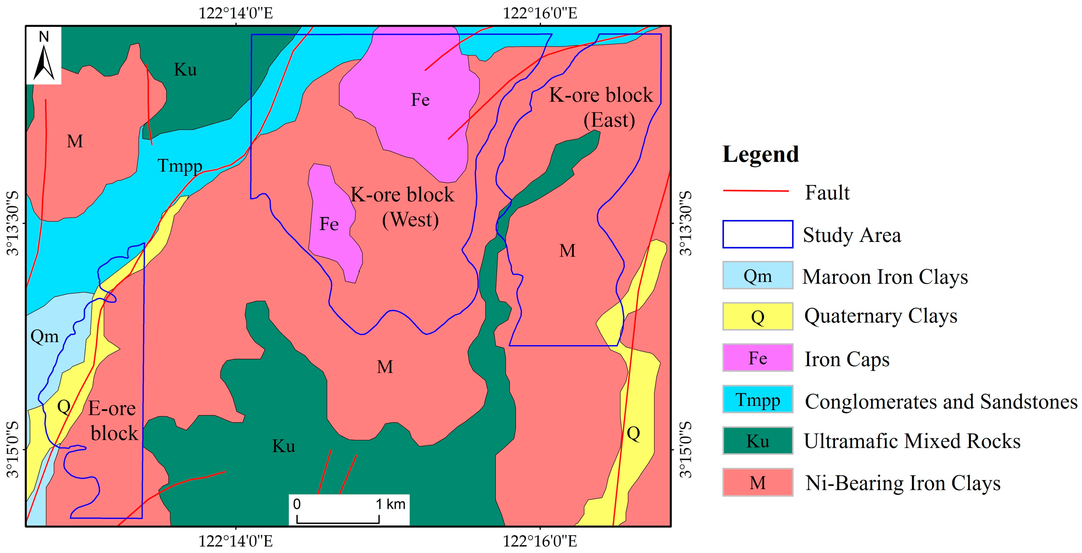
The study area encompasses Block E and K of the North Konawe Laterite Ni Zone, situated in Langgikima, North Konawe Regency, Sulawesi Province, Indonesia. It is geographically located between 122°12′41.809″E–122°16′47.556″E and 3°12′8.249″S–3°15′27.278″S, covering a total area of approximately 17.91 km² (Figure 1). This region experiences a tropical rainforest climate characterized by ample precipitation, high temperatures, and humidity. The landscape predominantly consists of hills and mountains near the coastal areas. The general topographic slope ranges from 10° and 25°, with certain localized sections exceeding 45°.
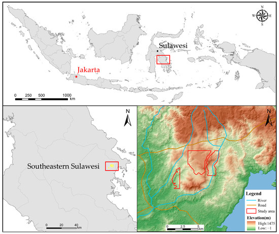
Figure 1.
Location map of the study area (Block E and K of the North Konawe Ni Deposit, Indonesia).
Within the study area exists extensive exposure of basal and ultramafic rocks at the surface. And a significant presence of brownish-red Ni-iron clay can be observed, accompanied by vast expanses of exposed ultramafic rocks such as peridotite and gabbro surrounding the ore body. However, the presence of lateritic weathering crust and forest cover constrains the visibility of tectonic traces within the mining area, thereby resulting in scarce overall tectonic information, such as faults, etc. (Figure 2). In summary, these natural geographic conditions and geological characteristics have served as a favorable foundation for the formation, enrichment, and preservation of lateritic Ni deposits.

Figure 2.
The geological map of North Konawe Ni Mining area.
2.2. Data
2.2.1. WordView-3 Remote Sensing Data
The WorldView-3 satellite, launched on 13 August 2014, represents the highest commercial optical satellites in terms of spatial resolution. It offers unrivaled capabilities for long-range mineral mapping and identification that are unmatched by any other multispectral satellite system available. This advanced satellite platform comprises one panchromatic band, eight visible-near-infrared (VNIR; 0.42–1.04 μm) multispectral bands, and eight short-wave infrared (SWIR; 1.2–2.33 μm) bands [67]. Although most studies in remote sensing geology rely on ASTER and ETM+ data, the eight SWIR bands of the WorldView-3 satellite demonstrate tremendous potential surpassing that of ASTER and ETM+ data. Hence, for this study, WorldView-3 data covering the study area were acquired from Earth Online. The dataset represents a single view acquired on November 1, 2019, exhibiting minimal cloud coverage to fulfill the requirements of the study.
2.2.2. Ni Grade Data
A comprehensive dataset consisting of 18,882 Ni grade samples was collected from the study area. The current ‘Chinese Code of Practice for Geological Exploration of Copper, Lead, Zinc, Silver, Ni, and Molybdenum Ores (DZ/T0214-2002)’ outlines the general industrial criteria for lateritic Ni ores. According to the code, the minimum industrial grade for Ni is set at 1.0%, while the Ni cut-off grade is 0.5%. Therefore, this study focused on Ni analysis, commencing from the cut-off grade as the baseline.
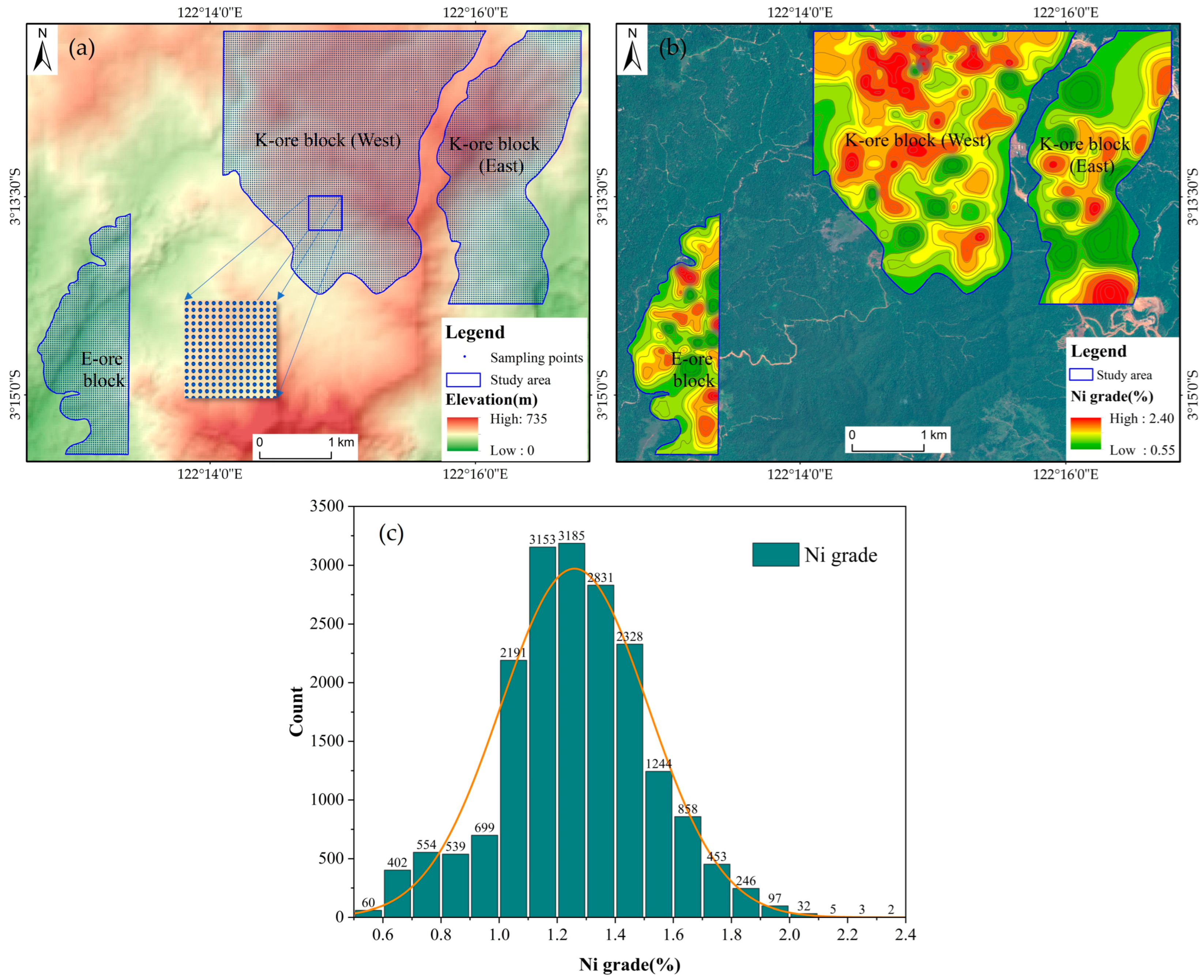
The highest, lowest, and average Ni grades within the study area were 2.40%, 0.55%, and 1.26%, respectively. The majority of Ni grades surpassed the industrial threshold of 1%, with distribution concentrated between 1.0% and 1.8%. Notably, the data exhibited spikes within the range of 1.2% to 1.3% (Figure 3). To ensure comprehensive analysis, the 18,882 sampling points, uniformly distributed across the study area, were randomly divided into two groups at an 8:2 ratio. Subsequently, 15,106 sampling points were allocated as the training group, while the remaining 3776 sampling points served as the validation group.
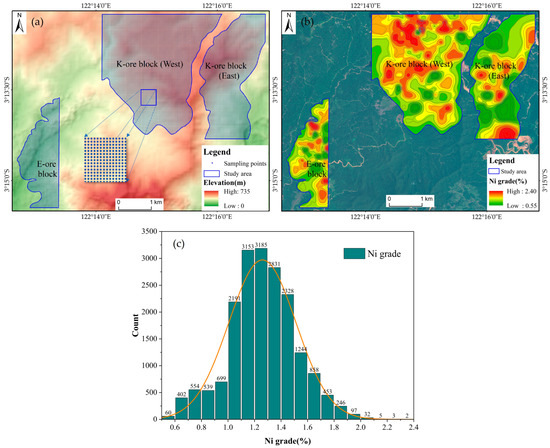
Figure 3.
(a) Distribution of Ni grade sampling points; (b) Ni grade contours; (c) histogram of measured Ni grade data.
2.3. Data Processing
2.3.1. Remote Sensing Data Preprocessing
By conducting radiation calibration, a quantitative relationship can be established between the digital quantization values of the image and their corresponding radiation brightness values in the field of view. This calibration process effectively mitigated radiation errors originating from the sensor itself. Even following radiometric calibration, the image data were still affected by atmospheric factors, necessitating atmospheric correction. The fast line-of-sight atmospheric analysis of spectral hypercubes (FLASSH) algorithm was applied to the VNIR and SWIR bands of WorldView-3 with the Tropical atmospheric model and the Rural aerosol model. And then, the VNIR and SWIR bands of WorldView-3 data were used for layer stacking. The SWIR bands with a spatial resolution of 3.7 m were resampled to match the VNIR bands with a resolution of 1.24 m through the cubic convolution method.
2.3.2. Band Preferred
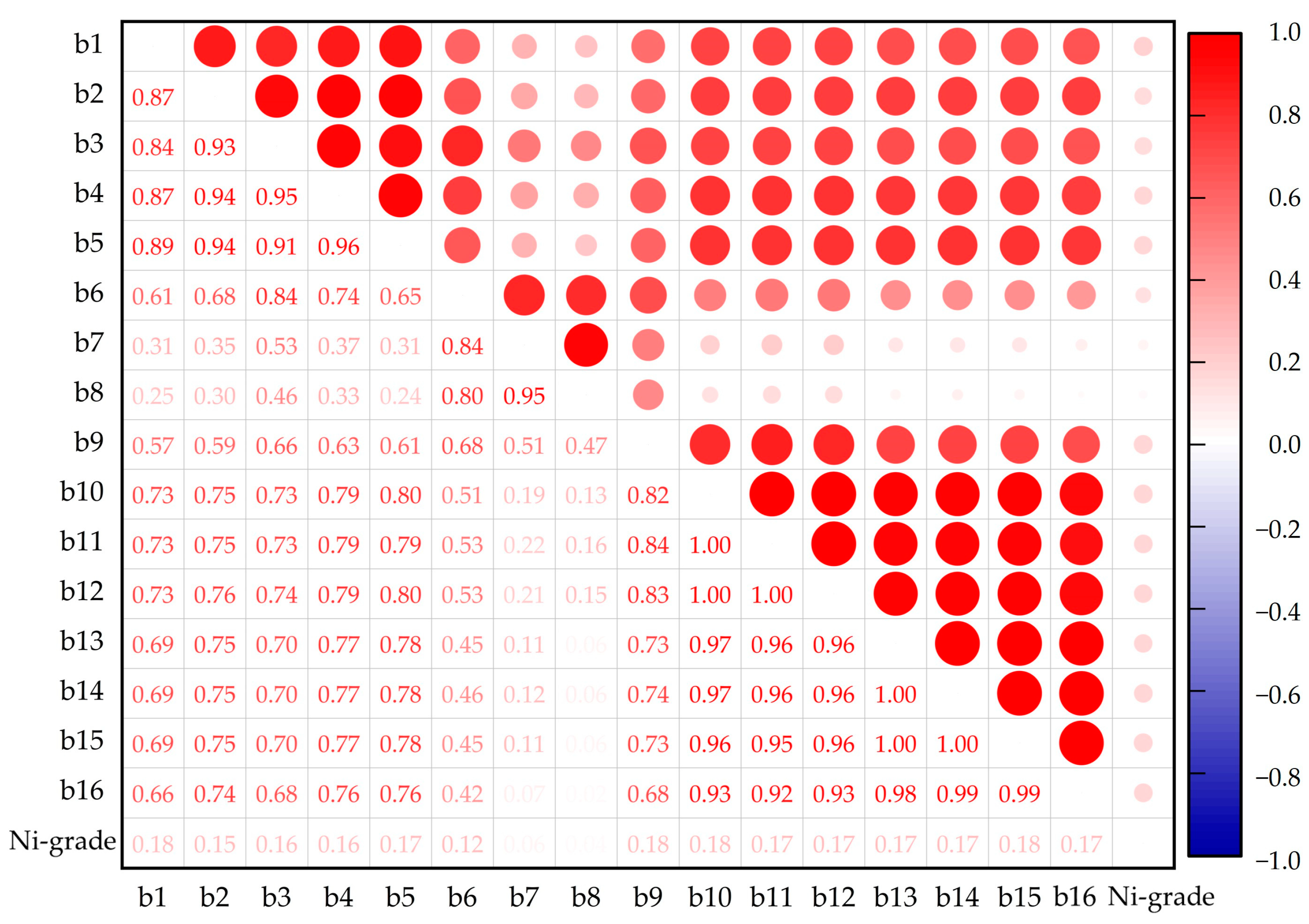
By examining the relationship between the band information of WorldView-3 data and the actual measured values of Ni grade in the study area, the band with higher correlation coefficient was identified for constructing the Ni grade inversion method. To mitigate the impact of magnitude differences on the results, the band information of WorldView-3 data was Z-Standardized prior to the calculation of the Spearman correlation coefficient with the Ni grade data (Figure 4). Given a sample size of n, n many raw data x and y were transformed into grade data, and the Spearman correlation coefficient (ρ) was calculated using Equation (1):

Figure 4.
Correlation analysis result between spectra and Ni grade measurements.
Utilizing the outcomes of the correlation analysis, the bands exhibiting high Spearman correlation coefficients and significant correlations at the 0.01 level were initially identified. Subsequently, the mean of correlation coefficients between the selected bands and the remaining bands were separately computed. Bands displaying high average correlation coefficients were subsequently excluded, while those with noteworthy correlations were retained for the development of the Ni grade inversion method.
The variance inflation factor (VIF) can be a useful metric for assessing the presence of multicollinearity among variables. A higher VIF value can indicate a stronger covariance between variables, which can be detrimental to the model-building process. Following the principle that the VIF value should be below 10 [68,69], the final selection of explanatory variables for this study comprised Band 1, Band 5, and Band 10 (Table 1).

Table 1.
Results of VIF between band 1, band 5, band 10, and band 15 for WorldView-3 data.
2.3.3. Spatial Autocorrelation Analysis of Ni Grades
Moran’s I is a statistical measure that evaluates the presence and intensity of spatial correlation among variables at various locations. A positive Moran’s I value (>0) indicates the presence of positive spatial correlation, with higher values indicating a stronger spatial correlation and a tendency for study unit observations to cluster together. Conversely, a negative Moran’s I value (<0) indicates negative spatial correlation, with smaller values indicating greater spatial variability and a tendency for study unit observations to be dispersed. When Moran’s I value equals zero (Moran’s I = 0), it suggests the absence of spatial autocorrelation, with study unit observations randomly distributed across space.
The computation of the Moran’s index (Equation (2)) was a prerequisite for the geographically weighted regression. The outcomes of the Moran’s index calculation (Table 2) revealed a positive spatial correlation among the Ni grades within the studied area. Furthermore, considering the z-score, the spatial autocorrelation of Ni grades in the study area can be regarded as statistically significant.
where denotes the spatial weight matrix; and represent the observations of i and j, respectively; and n denotes the number of spatial cells.

Table 2.
Results of spatial autocorrelation analysis of Ni grade data.
Based on the relevant criteria for GWR, it is evident that the analyzed objects exhibited substantial spatial autocorrelation and significant spatial heterogeneity. Hence, the application of the GWR model was deemed appropriate for the inversion study of Ni grades using World View-3 data (Table 2).
2.4. Inversion Methods
In this study, the inversion of Ni grades for the North Konawe laterite Ni ore in Indonesia was performed through the applications of MLR, BPNN, and GWR techniques. The preferred WorldView-3 data bands, namely Band 1, Band 5, and Band 10, were utilized as input variables for the inversion analysis.
2.4.1. MLR
The MLR emerges as a statistical technique applied for the establishment of regression equations that quantitatively explain the linear relationship between dependent and independent variables. Its fundamental concept can be adopted for seeking the most suitable mathematical expression that accurately represents the relationship between these variables [70]. Linear regression models consist of global and local models, where the global model assumes that the regression coefficients remain constant across all spatial locations within the study area, ensuring global consistency [71]. Among these models, MLR models have been widely employed as the conventional global models.
where Y represents the dependent variable; denote the independent variable; denotes the constant term; denote the regression coefficient; and e represents the random error term.
In this study, the dependent variable Y represented the Ni grade, and the independent variables X1, X2, and X3 can be regarded as the Band 1, Band 5, and Band 10 values of WorldView-3 data, respectively. The regression coefficients of the bands were solved by the least-squares method.
2.4.2. BPNN
The BPNN model is a widely adopted artificial neural network model, particularly in domains such as prediction and classification evaluations [72,73,74]. It consists of an input layer, a hidden layer, and an output layer. The underlying principle involves iteratively adjusting the network’s connection weights and thresholds during the mathematical transformation of the hidden layer. This adjustment can be achieved through the forward propagation of the input signal and the backward propagation of the output error, aiming to minimize the squared error between the actual output value and the desired output value [75,76,77].
where x denotes the input data; y denotes the output data; ω and b represent the weight matrix and bias vector of the adjacent layers, respectively; and f represents the activation function.
In this study, the input dataset consisted of the Band 1, Band 5, and Band 10 values extracted from WorldView-3 data, while the output dataset comprised the Ni grade. The BPNN employed in this study included three hidden layers, each comprising 30 neurons. The maximum number of iterations was set to 100, with a learning rate of 0.1. The desired network performance was defined as 0.00, and the Sigmoid function served as the chosen activation function. The implementation of the BPNN algorithm was conducted through Matlab programming language.
2.4.3. GWR
GWR incorporates the spatial location information of the data into the regression coefficients of the model, enabling the coefficients of the same variable to vary based on spatial location. This allows for the quantitative representation of the spatially heterogeneous characteristics inherent in the data. The fundamental expression of the GWR model is presented in Equation (5), which can capture the essence of this spatially adaptive regression approach.
where denotes the dependent variable; denote the spatial location of the i-th sample point; denote the intercept; denote the k-th regression coefficient of the i-th sample point; represents the k-th independent variable of the i-th sample point; represents the random error term; and represents the Ni grade of the i-th sample point in this study.
GWR can be described as a localized form of the least squares method [78,79], where the regression coefficients are adaptively determined based on the proximity of data points within a given spatial neighborhood. To characterize the decay of weights as the distance between data points increases, a spatial weight function can be employed [80]. Popular selections for spatial weight functions include the Gauss function, exponential function, and Bi-square function [81]. In this study, the Gauss function (Equation (6)) was employed to capture the spatial weighting scheme, enabling the analysis of localized relationships between variables.
where b denotes the bandwidth; denotes the distance between the sample points and the regression points; and denotes the weight of the sample points.
In this study, the GWR method incorporated Band 1, Band 5, and Band 10 values from WorldView-3 data as independent variables, while Ni grade served as the dependent variable. To capture the spatially varying relationships, a Gaussian kernel function was adopted as the locally weighted function, allowing for adaptive weighting of neighboring data points. The optimal bandwidth for the Gaussian kernel function was determined using the cross-validation method, ensuring robust and reliable parameter estimation.
2.4.4. Precision Evaluation Indicators
The determination coefficient −(R2) (Equation (7)), the residual sum of squares (RSS) (Equation (8)), the root mean square error (RMSE) (Equation (9)), and the residual ε (Equation (10)) were statistical metrics employed to quantitatively evaluate the accuracy and stability of the inversion results [82]. These metrics can provide valuable insights into the goodness-of-fit, variability, and predictive performance of the Ni grade inversion model.
(1) R2
R2 measured the proportion of the total variation in the dependent variable explained by the model, with a value closer to 1 indicating better model stability.
(2) RSS
The RSS was applied as a measure of the difference between the sample data and the model predictions, where a smaller RSS indicated a better fit of the model.
(3) RMSE
(4) Residual-ε
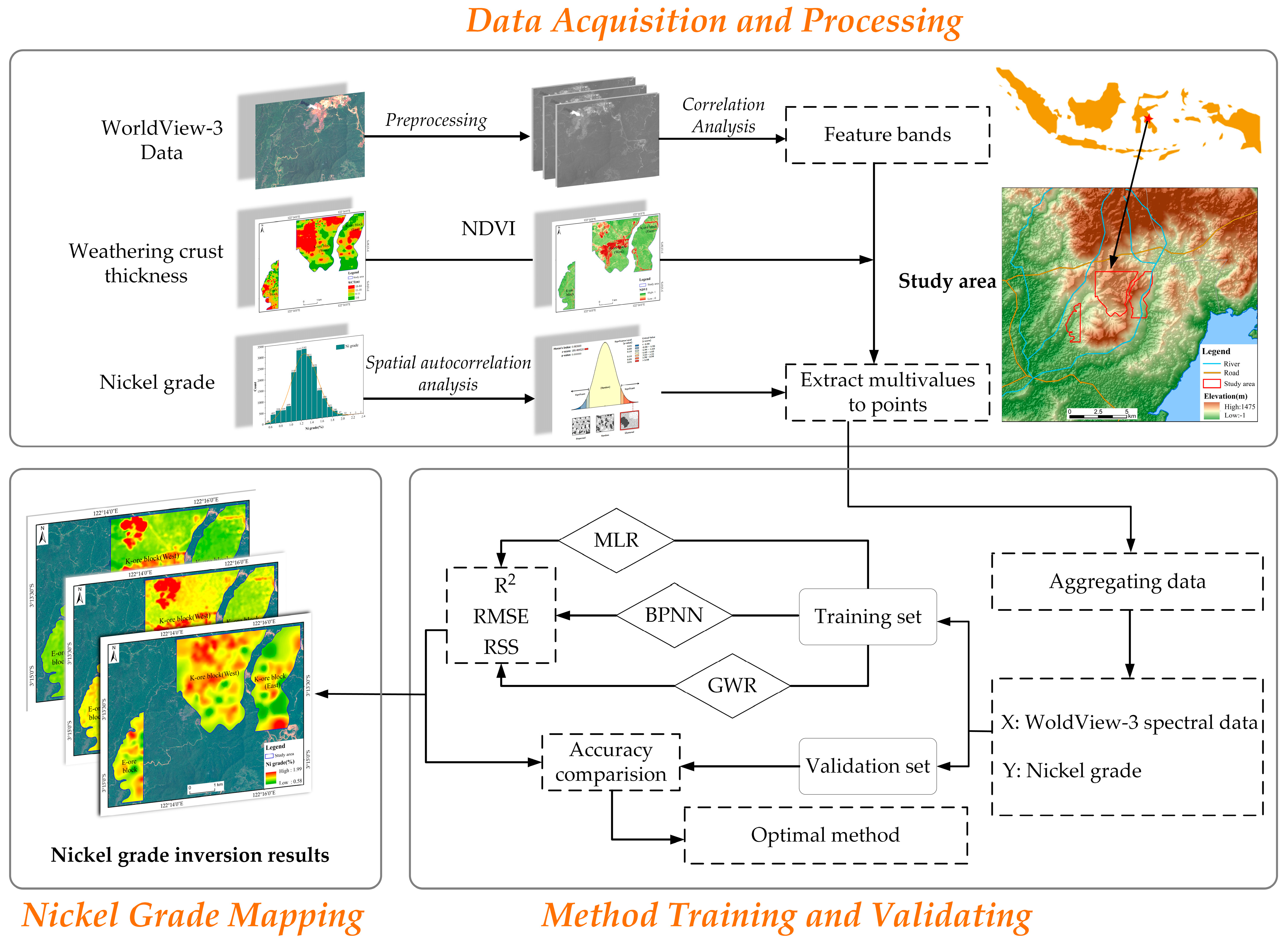
where n denotes the number of sampling points; denotes the measured Ni grade at the sampling points; denotes the predicted Ni grade at the sampling points; and represents the mean value of the measured Ni grade at the sampling points. In addition, the predicted and measured values were linearly fitted to verify the accuracy of the three methods in the Ni grade inversion study (Figure 5).
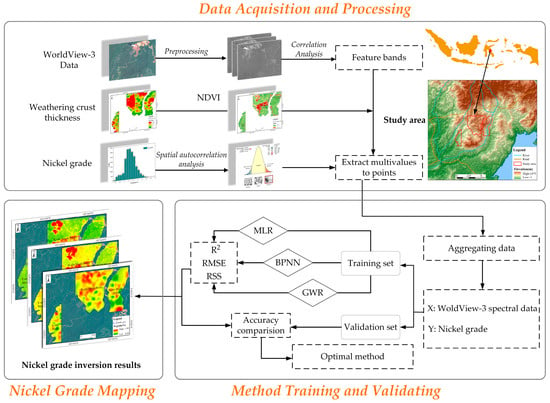
Figure 5.
Flowchart of the study.
3. Results
3.1. Spatial Distribution of Ni Grades and Accuracy Evaluation
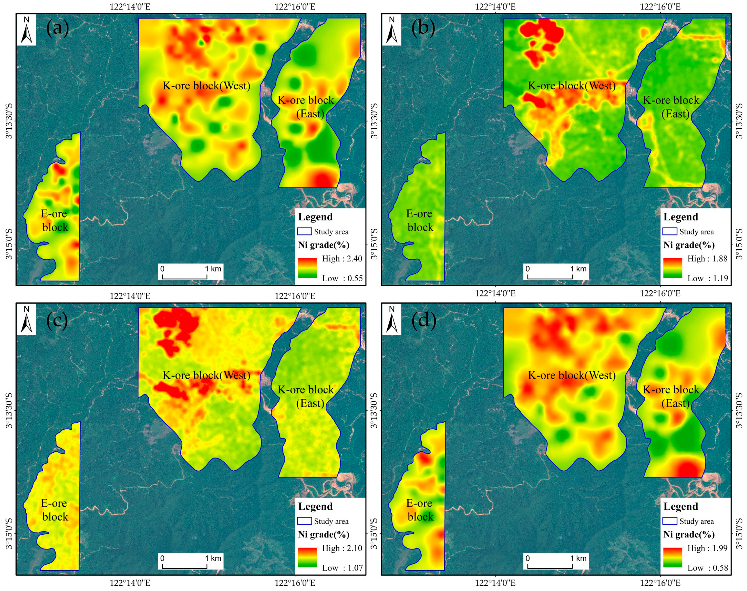
When comparing with the spatial distribution of the measured Ni grade data, it is observed that the regional variation of the Ni grade inversion values through MLR and BPNN was relatively uniform within the east ore body of block E and K. The differentiation of the inversion values at varying locations was not significantly evident. However, within the west ore body of block K, there was a distinct abrupt transition from high inversion values to low inversion values, indicating a notable variation. Notably, the inversion effect was more favorable in the exposed area, where the accuracy and reliability of the inversion results were comparatively higher.
The Ni grade prediction results based on GWR exhibited a remarkable agreement with the measured data in terms of the overall trend distribution, as well as the distribution of enrichment centers. However, certain minor discrepancies were observed in the periphery of local enrichment centers when compared to the measured data, indicating a slight diffusion effect (Figure 6).
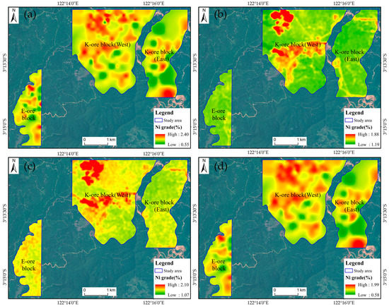
Figure 6.
(a) Measured Ni grade; (b) MLR inversion results; (c) BPNN inversion results; (d) GWR inversion results.
The three aforementioned methods demonstrated varying levels of performance in the inversion of Ni grades. MLR and BPNN exhibited poor performance, yielding R2 values of 0.05 and 0.17, respectively, as well as RMSE values of 0.25 and 0.23. In contrast, GWR, leveraging the spatial location information of the sample data, indicated the greatest advantages in Ni grade inversion, achieving the highest R2 value of 0.96 and the lowest RMSE value of 0.039. Additionally, the RSS of GWR was significantly smaller than that of MLR and BPNN (Table 3).

Table 3.
Comparison of MLR, BPNN, GWR for analysis of WorldView-3 data and Ni grade measurement.
To summarize, MLR demonstrated the lowest inversion accuracy, followed by BPNN, while GWR exhibited the highest accuracy, with an R2 value exceeding 0.95 and an RSS of only 47.22. The inclusion of Band 1, Band 5, and Band 10 from World View-3 data enabled the explanation of over 95% of the variation in Ni grades.
3.2. Comparison of Inversion Accuracy
3.2.1. Measured Value-Inversion Value Fitting
The inversion values obtained from MLR, BPNN, and GWR were subjected to linear fitting to the measured values (Figure 7). In Figure 7, the black line represents the fitted straight line connecting the measured and inverse values, while the orange line represents the function y=x with a slope of 1. The proximity of the sample points to the fitted straight line, as well as the angle between the fitted straight line and the line y = x, serve as the metrics of the regression accuracy of the method. The closer the sample points align with the fitted straight line and the smaller the angle between the fitted line and the line y = x, the higher the regression accuracy of the method is.

Figure 7.
Linear regression of measured and inversion Ni grade: (a) MLR; (b) BPNN; (c) GWR.
The angle between the fitted straight line connecting the inverse and measured values and the line y = x was large for both multiple linear regression and BPNN, suggesting that these two methods exhibited poor performance in the process of Ni grade inversion and lacked accuracy.
The fitted straight line representing the relationship between the inverse and measured Ni grades obtained through the GWR method exhibited slopes and R2 values of 0.902 and 0.965, respectively. Remarkably, the fitted straight line of GWR closely aligned with the y = x line, indicating that GWR significantly enhanced the accuracy of the fitted results. Therefore, GWR was highly appropriate for establishing the regression relationship between Ni grades and WordView-3 data, specifically Band 1, Band 5, and Band 10.
3.2.2. Residual Statistics
The residuals of MLR and BPNN exhibited a distribution range from −0.8 to 1.2, with a concentration between −0.4 and 0.4. Conversely, the residuals of GWR were concentrated within the narrow range of −0.1 to 0.1, with only a few sample points displaying absolute residuals exceeding 0.2. As depicted in Figure 8, GWR performed better than MLR and BPNN in terms of accuracy, as it successfully inverted the Ni grade within the study area while maintaining residuals within the permissible error range. The superior accuracy of GWR was evident when compared to the other two methods, MLR and BPNN.

Figure 8.
Residual statistics of three inversion methods: (a) MLR; (b) BPNN; (c) GWR.
3.3. Field Validation
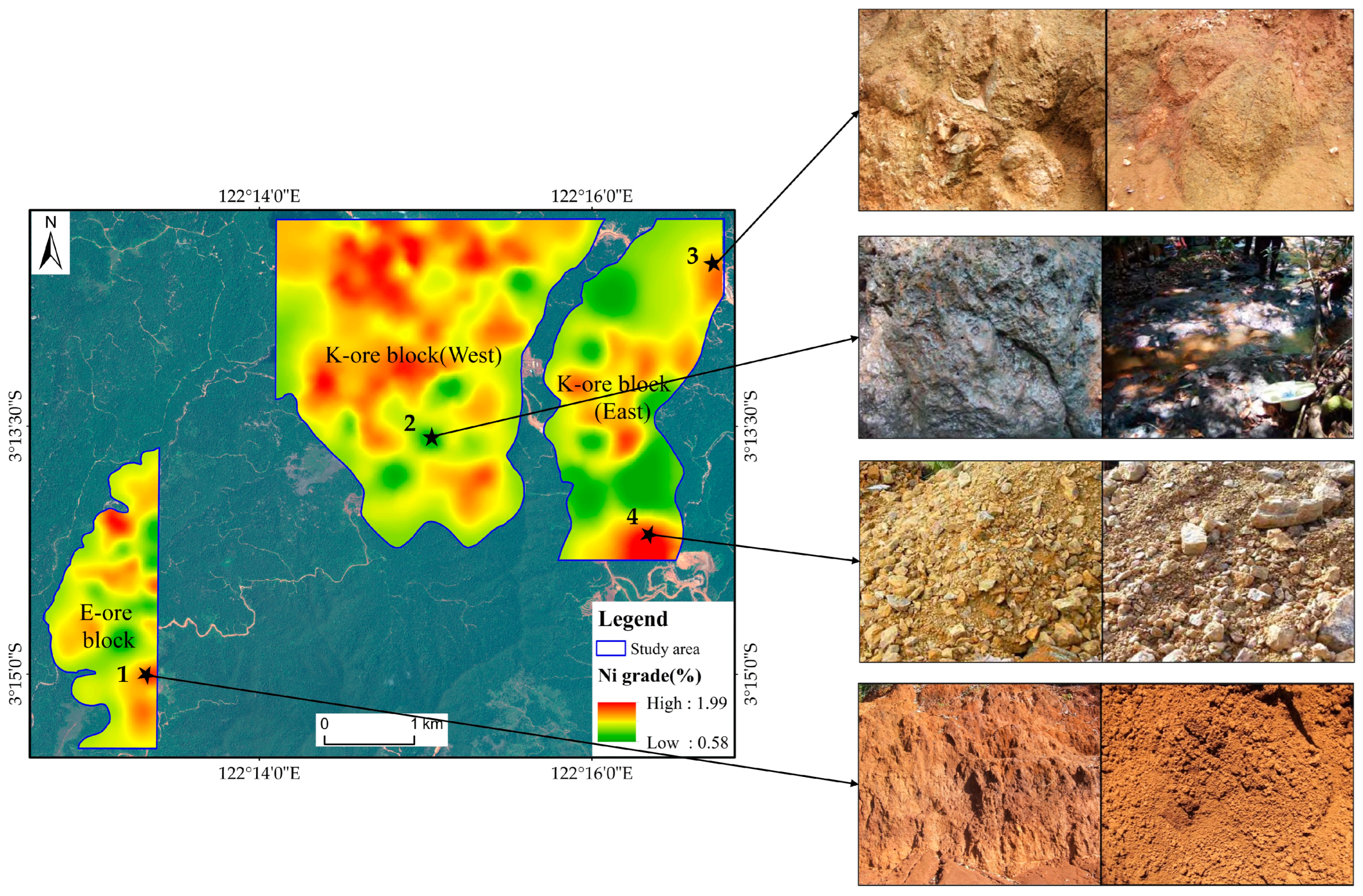
After conducting an accuracy comparison analysis, it was determined that GWR outperformed other methods in the inversion of Ni grade in laterite Ni ore. Consequently, field validation work was conducted on the inversion results obtained from GWR (Figure 9). Four validation points were selected, representing a range of Ni grades from low to high. Field measurements yielded Ni grades of 1.69, 0.98, 1.50, and 2.01 for soil samples No. 1, No. 2, No. 3, and No. 4, respectively. The inversion results exhibited a consistent trend with the field-measured data (Table 4).
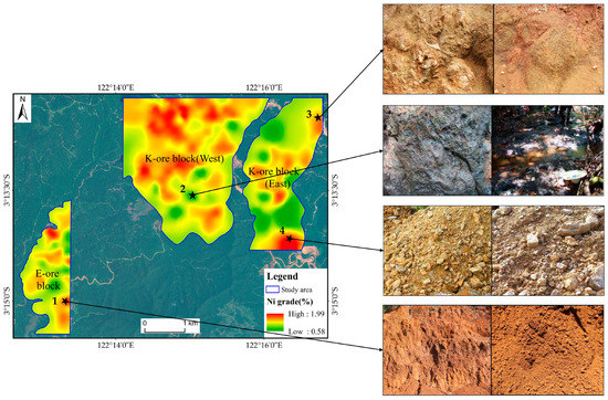
Figure 9.
Distribution of field validation sites.

Table 4.
Ni grade sampling point verification results.
4. Discussions
4.1. Spatial Distribution of GWR Inversion Values
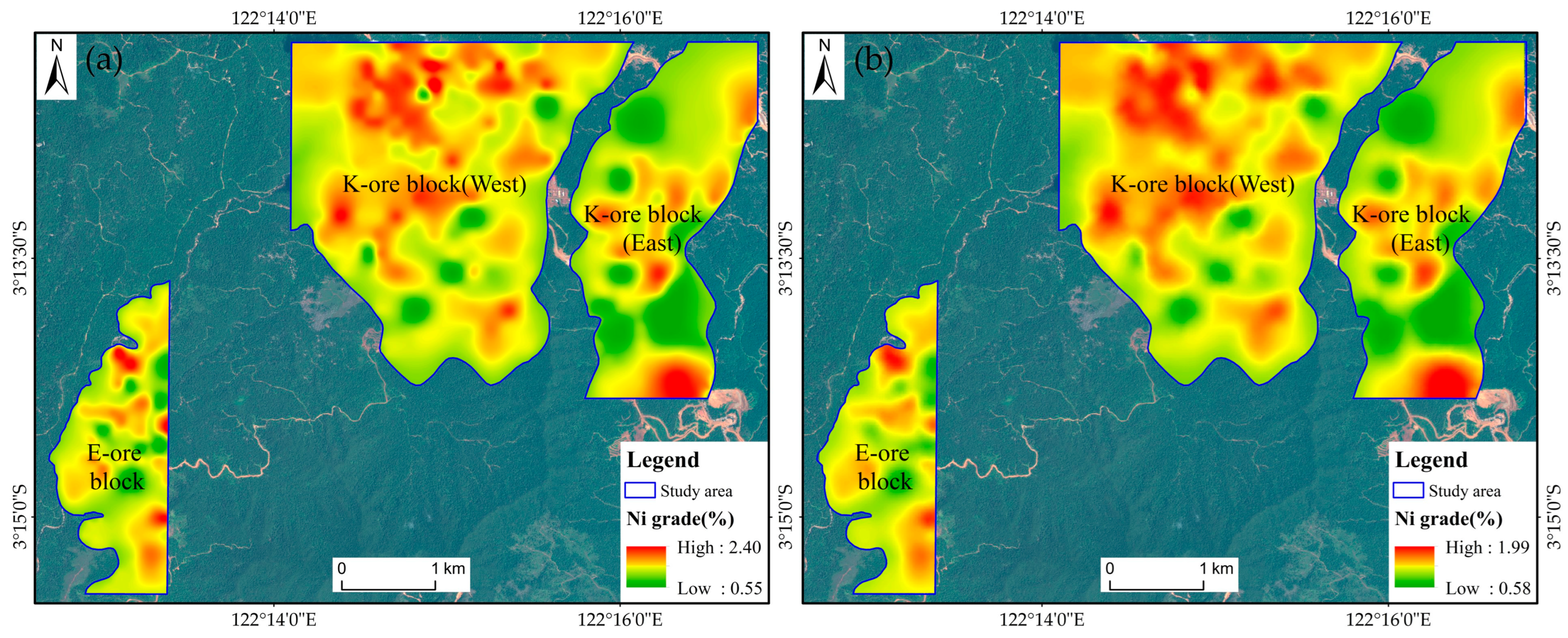
The study area exhibited a range of measured Ni grades, with the highest value recorded as 2.40, the lowest value as 0.55, and a mean value of 1.260. In contrast, the GWR inversion results for Ni grade indicated a narrower range, with the highest value reaching only 1.99, the lowest value at 0.58, and a mean value of 1.259 (Figure 10). Overall, while GWR demonstrated an ability to accurately predict the overall spatial distribution trend of Ni grades, it tended to slightly underestimate high Ni grade values and presented limited performance for extreme values when compared to the measured data.
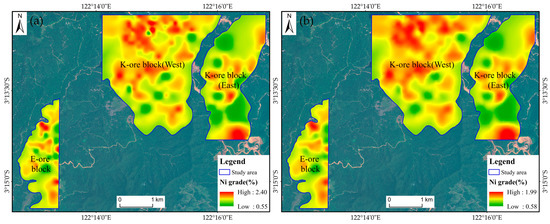
Figure 10.
(a) Measured Ni grade; (b) GWR inversion value of Ni grade.
4.2. Spatial Heterogeneity
The GWR methodology incorporated spatial location information of sampled points, enabling the characterization of spatial relationships with varying coefficients.
The coefficient plots (Figure 11) exhibited localized shading, with the intensity of the shades corresponding to the magnitude of the coefficient values. These coefficients presented the degree of correlation between each explanatory variable and Ni grade [83]. By considering the spatial proximity of the sample points, GWR derived variable coefficients at each interpolated location using neighboring sample points. The coefficient plots reflected an additional perspective, demonstrating that GWR was capable of capturing finer details of the spatial distribution of Ni grades and highlighting the spatial heterogeneity present in the Ni grade data.

Figure 11.
Coefficients of WorldView-3 bands obtained by GWR: (a) Band 1; (b) Band 5; (c) Band 10.
4.3. Influence Factors of Inversion
4.3.1. Degree of Weathering
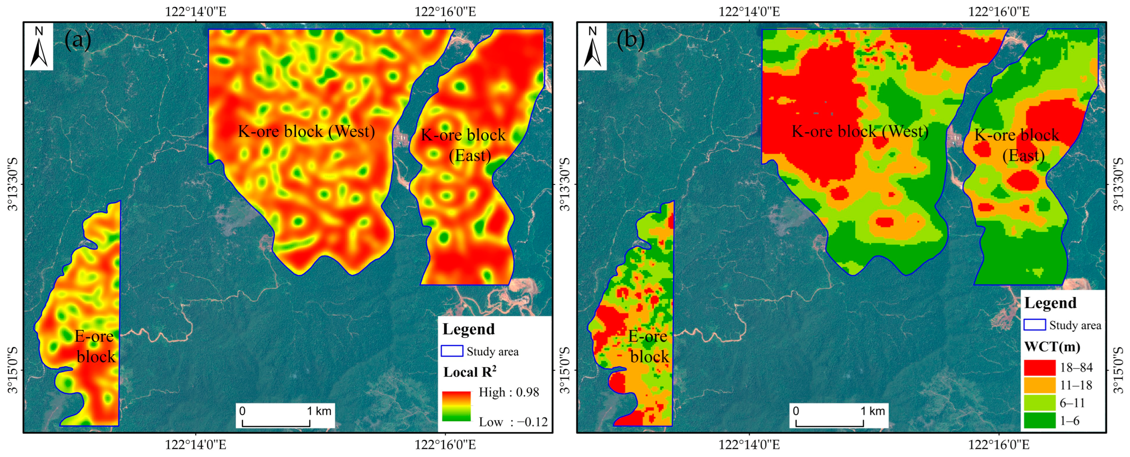
The accuracy of GWR inversion can be influenced by the weathering degree of the lateritic weathering crust. Previous studies have indicated a clear relationship between the degree of weathering and the enrichment of Ni. Specifically, Ni enrichment gradually increased from the laterite zone to the saprolite zone, with the highest enrichment observed in the upper part of the saprolite zone. In this study, the quartiles of weathering crust thickness values in the study area were calculated. The first, second, and third quartiles were determined as 6 m, 11 m, and 18 m, respectively, while the minimum and maximum values were 1 m and 84 m, respectively. According to this as the threshold, the local R2 values corresponding to different intervals of weathering crust thickness were computed separately (Table 5 and Figure 12).

Table 5.
Local R2 of GWR corresponding to different weathering crust thickness intervals.

Figure 12.
(a) GWR local R2; (b) weathering crust thickness (WCT) in the study area.
From a statistical standpoint, the local R2 values of GWR exhibited a gradual decline as the weathering crust thickness increased. The GWR method demonstrated the highest level of fit when the weathering degree was the weakest. This observation led to a reasonable inference that, as the degree of weathering intensified, the Ni element reached its maximum enrichment at deeper levels. Consequently, the spectral response weakened, resulting in a decrease in the accuracy of GWR inversion. Therefore, the spectral response mechanism of Ni elements was intricately linked to the degree of laterite weathering.
4.3.2. Vegetation Coverage
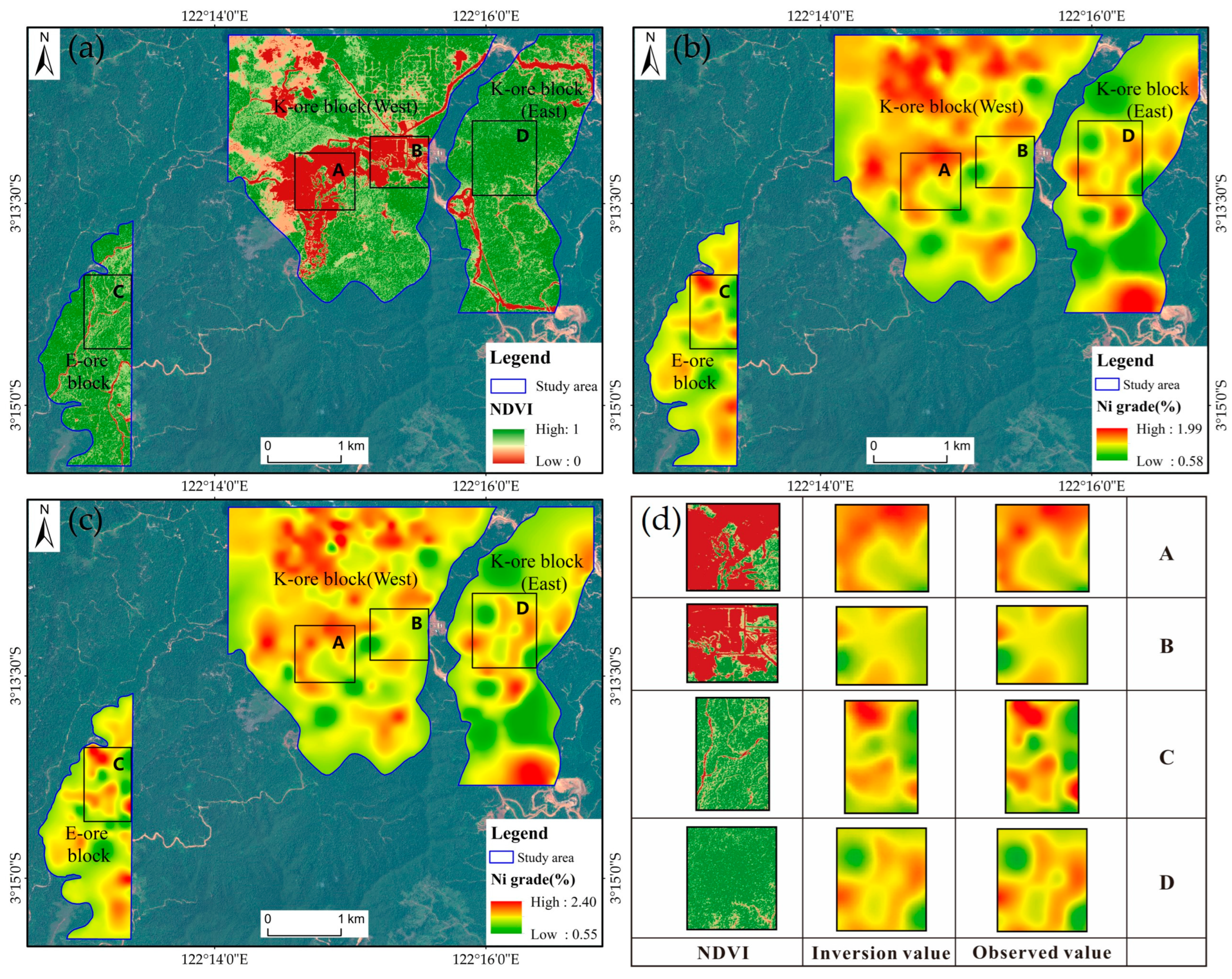
It was observed that the prediction accuracy varied across different areas, with vegetation cover being one of the contributing factors. The areas with high vegetation cover exhibited relatively poor prediction performance. To investigate this further, four distinct areas were selected based on the normalized difference vegetation index (NDVI) results: two areas with low vegetation cover (A and B) and two areas with high vegetation cover (C and D) (Figure 13). The spatial distribution trends of the GWR inversion Ni grades in these four regions were generally consistent with the measured values. However, in regions C and D, where there was a transition from high to low Ni grade values, the inversion results exhibited inadequacies, with a lack of precision in capturing local variations compared to the measured values.

Figure 13.
(a) NDVI; (b) GWR inversion value of Ni grade; (c) measured value of Ni grade; (d) regions of interest.
The NDVI values and corresponding local R2 values were computed for four representative areas, namely A, B, C, and D (Table 6). The average local R2 value in regions A and B was 0.80, which was higher than the value in regions C and D (0.76). Within the transition interval from areas with low to high vegetation cover, the local R2 of GWR decreased from 0.82 to 0.74 as the NDVI presented an increasing trend. However, it was observed that the trend of local R2 with NDVI within areas of high and low vegetation cover was inconsistent with the trend observed within the transition interval.

Table 6.
NDVI and local R2 for the four regions of interest.
Hence, a reasonable inference can be concluded that vegetation coverage exerted a significant influence on the spectral response of Ni grade, resulting in a decrease in inversion accuracy. However, the precise internal correlations between vegetation coverage and the spectral response of Ni grade remained unclear, necessitating further analysis and research to elucidate the underlying mechanisms governing the influence of vegetation coverage on the inversion of Ni grade.
In conclusion, the spatial distribution trend of the overall Ni grade inversion resulted in the study area, based on GWR, exhibited consistency with the measured values. However, certain sections indicated certain limitations in accurately inversing Ni grade due to the impact of vegetation cover and laterite weathering degree. Furthermore, the exclusion of lithology as a variable in the GWR analysis restricted the performance. Therefore, further exploration is required to investigate how to effectively incorporate the categorical variable of lithology into the GWR method, aiming to unravel its intrinsic association with Ni grade.
5. Conclusions
This study revealed the remarkable capability of Band 1, Band 5, and Band 10 from WorldView-3 remote sensing data, combined with the locally weighted regression method GWR, that can accurately inverse the Ni grade of lateritic Ni ore. The findings unequivocally demonstrated that GWR effectively captured the intricate local variations in Ni grades within the study area, providing a more comprehensive and scientifically sound depiction compared to MLR and BPNN. Notably, the inclusion of location information resulted in a substantial enhancement in the accuracy of Ni grade inversion, with R2 increasing from a mere 0.17 to surpass 0.9. Thus, it can be proved that a robust relationship between Ni grade and WorldView-3 remote sensing data was observed in the North Konawe Ni ore area, emphasizing the significant impact of geospatial location.
The investigation revealed a direct correlation between the weathering degree of lateritic weathered crust and the spectral response of Ni elements. Specifically, as the weathering degree increased, the depth of Ni enrichment intensified, consequently resulting in a decline in inversion accuracy. Moreover, vegetation cover exerted a detrimental effect on the inversion of Ni grade by restricting the value range of inversion results. Notably, the accuracy of inversion was notably reduced in the transitional regions between high and low values of Ni grade. However, the precise mechanism underlying this impact necessitated further analysis and research.
The GWR method employed in this study demonstrated excellent performance in the inversion of Ni grades in lateritic Ni ores, even in the absence of geological data and prior information in the study area. Nevertheless, certain limitations still remained, necessitating the collection of more comprehensive geological information in future investigations. Moreover, it is recommended to incorporate the lithology of the study area to enhance the accuracy of inversion results.
Author Contributions
Conceptualization, G.Z., Q.C. and Z.Z.; data curation, G.Z. and Q.C.; formal analysis, Z.L., X.Z.; methodology, G.Z., X.Z. and J.C.; software, G.Z., Y.H. and D.Z.; resources, Z.Z.; investigation, W.C. and H.Y.; validation, D.Z., H.Y. and J.C.; funding acquisition, Z.Z.; visualization, Y.H. and Z.L.; writing—original draft preparation, G.Z. and Q.C.; writing—review and editing, Z.Z., Q.C. and D.Z. All authors have read and agreed to the published version of the manuscript.
Funding
This research was funded by “Yunnan International Joint Laboratory of China-Laos-Bangladesh-Myanmar Natural Resources Remote Sensing Monitoring” (Grant No. 202303AP140015), “National Natural Science Foundation of China” (Grant No. 41872251), “National Natural Science Foundation of China” (Grant No. 42202329), “Science and Technology Plan Project of Yunnan Province Science and Technology Department” (Grant No. 202101BA070001-145), “The 14th Graduate Research Innovation Project” (Grant No. KC-22223390), “Yunnan Provincial Department of Education Science Research Fund Project” (Grant No. 2023Y0196).
Data Availability Statement
The data presented in this study are available upon request from the corresponding author.
Acknowledgments
The authors would like to thank Unit 308 of Yunnan Nonferrous Geology Bureau for the data support and the anonymous reviewers for their valuable comments on the manuscript.
Conflicts of Interest
The authors declare no conflict of interest.
References
- Hou, Z.; Chen, J.; Zhai, M. Current status and frontiers of research on critical mineral resources. Kexue Tongbao (Chin. Ed.) 2020, 65, 3651–3652. [Google Scholar] [CrossRef]
- Lu, Y.; Lesher, C.M.; Deng, J. Geochemistry and genesis of magmatic Ni-Cu-(PGE) and PGE-(Cu)-(Ni) deposits in China. Ore Geol. Rev. 2019, 107, 863–887. [Google Scholar] [CrossRef]
- Butt, C.R.M.; Cluzel, D. Nickel Laterite Ore Deposits: Weathered Serpentinites. Elements 2013, 9, 123–128. [Google Scholar] [CrossRef]
- Valeton, I.; Biermann, M.; Reche, R.; Rosenberg, F. Genesis of nickel laterites and bauxites in Greece during the Jurassic and Cretaceous, and their relation to ultrabasic parent rocks. Ore Geol. Rev. 1987, 2, 359–404. [Google Scholar] [CrossRef]
- Apostolikas, T.; Frogoudakis, E.; Bakalllbashi, J. Nickel, World Production and Demand. In Proceedings of the 3rd Balkan Mining Congress, Book of Proceedings, İzmir, Turkey, 1–3 October 2009. [Google Scholar]
- Zeng, X.; Xu, H.; Tian, Y.; Liu, Z.; Li, M. Situation and sustainable development strategy of China’s nickel resources industry. Resour. Ind. 2015, 17, 94–99. [Google Scholar]
- Nieto, A. The Strategic Importance of Nickel: Scenarios and Perspectives Aimed to Global Supply. J. Min. Metall. B 2013, 332, 510–518. [Google Scholar]
- Dalvi, A.; Bacon, W.; Osborne, R. The Past and the Future of Nickel Laterites. In Proceedings of the PDAC 2004 International Convention, Trade Show & Investors Exchange, Toronto, ON, Canada, 7–10 March 2004; The Prospectors and Developers Association of Canada: Toronto, ON, Canada, 2004. [Google Scholar]
- Zuo, R.; Wang, J.; Xiong, Y.; Wang, Z. The processing methods of geochemical exploration data: Past, present, and future. Appl. Geochem. 2021, 132, 105072. [Google Scholar] [CrossRef]
- Hou, L.; Li, X.; Li, F. Hyperspectral-based Inversion of Heavy Metal Content in the Soil of Coal Mining Areas. J. Environ. Qual. 2019, 48, 57–63. [Google Scholar] [CrossRef] [PubMed]
- Mao, Y.; Liu, J.; Cao, W.; Ding, R.; Fu, Y.; Zhao, Z. Research on the quantitative inversion model of heavy metals in soda saline land based on visible-near-infrared spectroscopy. Infrared Phys. Technol. 2021, 112, 103602. [Google Scholar] [CrossRef]
- Golightly, J. Progress in understanding the evolution of nickel laterites. In The Challenge of Finding New Mineral Resources: Global Metallogeny, Innovative Exploration, and New Discoveries; Goldfarb, R.J., Marsh, E.E., Monecke, T., Eds.; Society of Economic Geologists: Littleton, CO, USA, 2010; Volume 15, pp. 451–485. [Google Scholar]
- Lyu, P.; He, L.; He, Z.; Liu, Y.; Deng, H.; Qu, R.; Wang, J.; Zhao, Y.; Wei, Y. Research on remote sensing prospecting technology based on multi-source data fusion in deep-cutting areas. Ore Geol. Rev. 2021, 138, 104359. [Google Scholar] [CrossRef]
- Abulghasem, Y.A.; Akhir, J.B.M.; Hassan, W.F.W.; Samsudin, A.R.; Youshah, B.M. The use of remote sensing technology in geological investigation and mineral detection in Wadi shati, Libya. Electron. J. Geotech. Eng. 2012, 17 I, 1279–1291. [Google Scholar]
- Shi, T.; Chen, Y.; Liu, Y.; Wu, G. Visible and near-infrared reflectance spectroscopy—An alternative for monitoring soil contamination by heavy metals. J. Hazard. Mater. 2014, 265, 166–176. [Google Scholar] [CrossRef] [PubMed]
- Shi, T.; Liu, H.; Chen, Y.; Wang, J.; Wu, G. Estimation of arsenic in agricultural soils using hyperspectral vegetation indices of rice. J. Hazard. Mater. 2016, 308, 243–252. [Google Scholar] [CrossRef]
- Ibrahim, E.; Barnabé, P.; Ramanaidou, E.; Pirard, E. Mapping mineral chemistry of a lateritic outcrop in new Caledonia through generalized regression using Sentinel-2 and field reflectance spectra. Int. J. Appl. Earth Obs. Geoinf. 2018, 73, 653–665. [Google Scholar] [CrossRef]
- Seoane, J.C.; Castro, N.; Osako, L.; Baars, F. Multispectral Imagery Applied to Nickel Laterite Exploration: The Conceição do Araguaia Discovery. Rev. Econ. Geol. 2009, 16, 109–122. [Google Scholar]
- Wells, M.A.; Chia, J. Quantification of Ni laterite mineralogy and composition: A new approach. Aust. J. Earth Sci. 2011, 58, 711–724. [Google Scholar] [CrossRef]
- Yang, K.; Whitbourn, L.; Mason, P.; Huntington, J. Mapping the Chemical Composition of Nickel Laterites with Reflectance Spectroscopy at Koniambo, New Caledonia. Econ. Geol. 2013, 108, 1285–1299. [Google Scholar] [CrossRef]
- Basile, A.; Hughes, J.; McFarlane, A.J.; Bhargava, S.K. Development of a model for serpentine quantification in nickel laterite minerals by infrared spectroscopy. Miner. Eng. 2010, 23, 407–412. [Google Scholar] [CrossRef]
- Van der Meer, F. Near-infrared laboratory spectroscopy of mineral chemistry: A review. Int. J. Appl. Earth Obs. Geoinf. 2018, 65, 71–78. [Google Scholar] [CrossRef]
- Farrokhpay, S.; Filippov, L.; Fornasiero, D. Pre-concentration of nickel in laterite ores using physical separation methods. Miner. Eng. 2019, 141, 105892. [Google Scholar] [CrossRef]
- Al-Khirbash, S.A. Mineralogical characterization of low-grade nickel laterites from the North Oman Mountains: Using mineral liberation analyses—Scanning electron microscopy-based automated quantitative mineralogy. Ore Geol. Rev. 2020, 120, 103429. [Google Scholar] [CrossRef]
- Lypaczewski, P.; Rivard, B.; Gaillard, N.; Perrouty, S.; Piette-Lauzière, N.; Bérubé, C.L.; Linnen, R.L. Using hyperspectral imaging to vector towards mineralization at the Canadian Malartic gold deposit, Québec, Canada. Ore Geol. Rev. 2019, 111, 102945. [Google Scholar] [CrossRef]
- Chen, Q.; Xia, J.; Zhao, Z.; Zhou, J.; Zhu, R.; Zhang, R.; Zhao, X.; Chao, J.; Zhang, X.; Zhang, G. Interpretation of hydrothermal alteration and structural framework of the Huize Pb–Zn deposit, SW China, using Sentinel-2, ASTER, and Gaofen-5 satellite data: Implications for Pb–Zn exploration. Ore Geol. Rev. 2022, 150, 105154. [Google Scholar] [CrossRef]
- Pour, A.B.; Hashim, M.; van Genderen, J. Detection of hydrothermal alteration zones in a tropical region using satellite remote sensing data: Bau goldfield, Sarawak, Malaysia. Ore Geol. Rev. 2013, 54, 181–196. [Google Scholar] [CrossRef]
- Chen, Q.; Zhao, Z.; Zhou, J.; Zhu, R.; Xia, J.; Sun, T.; Zhao, X.; Chao, J. ASTER and GF-5 Satellite Data for Mapping Hydrothermal Alteration Minerals in the Longtoushan Pb-Zn Deposit, SW China. Remote Sens. 2022, 14, 1253. [Google Scholar] [CrossRef]
- Zhang, S.; Shen, Q.; Nie, C.; Huang, Y.; Wang, J.; Hu, Q.; Ding, X.; Zhou, Y.; Chen, Y. Hyperspectral inversion of heavy metal content in reclaimed soil from a mining wasteland based on different spectral transformation and modeling methods. Spectrochim. Acta A Mol. Biomol. Spectrosc. 2019, 211, 393–400. [Google Scholar] [CrossRef]
- Shen, Q.; Xia, K.; Zhang, S.; Kong, C.; Hu, Q.; Yang, S. Hyperspectral indirect inversion of heavy-metal copper in reclaimed soil of iron ore area. Spectrochim. Acta A Mol. Biomol. Spectrosc. 2019, 222, 117191. [Google Scholar] [CrossRef]
- Adiri, Z.; Lhissou, R.; El Harti, A.; Jellouli, A.; Chakouri, M. Recent advances in the use of public domain satellite imagery for mineral exploration: A review of Landsat-8 and Sentinel-2 applications. Ore Geol. Rev. 2020, 117, 103332. [Google Scholar] [CrossRef]
- Abrams, M.; Yamaguchi, Y. Twenty Years of ASTER Contributions to Lithologic Mapping and Mineral Exploration. Remote Sens. 2019, 11, 1394. [Google Scholar] [CrossRef]
- Krupnik, D.; Khan, S. Close-range, ground-based hyperspectral imaging for mining applications at various scales: Review and case studies. Earth Sci. Rev. 2019, 198, 102952. [Google Scholar] [CrossRef]
- Longbotham, N.; Pacifici, F.; Malitz, S.; Baugh, W.; Camps-Valls, G. Measuring the Spatial and Spectral Performance of WorldView-3. In Proceedings of the Fourier Transform Spectroscopy and Hyperspectral Imaging and Sounding of the Environment, Lake Arrowhead, CA, USA, 1 March 2015; p. HW3B.2. [Google Scholar]
- Ye, B.; Tian, S.; Ge, J.; Sun, Y. Assessment of WorldView-3 Data for Lithological Mapping. Remote Sens. 2017, 9, 1132. [Google Scholar] [CrossRef]
- Li, D.; Ke, Y.; Gong, H.; Li, X. Object-Based Urban Tree Species Classification Using Bi-Temporal WorldView-2 and WorldView-3 Images. Remote Sens. 2015, 7, 16917–16937. [Google Scholar] [CrossRef]
- Kruse, F.A.; Perry, S.L. Mineral Mapping Using Simulated Worldview-3 Short-Wave-Infrared Imagery. Remote Sens. 2013, 5, 2688–2703. [Google Scholar] [CrossRef]
- Song, L.; Jian, J.; Tan, D.-J.; Xie, H.-B.; Luo, Z.-F.; Gao, B. Estimate of heavy metals in soil and streams using combined geochemistry and field spectroscopy in Wan-sheng mining area, Chongqing, China. Int. J. Appl. Earth Obs. Geoinf. 2015, 34, 1–9. [Google Scholar] [CrossRef]
- Guan, Q.; Zhao, R.; Wang, F.; Pan, N.; Yang, L.; Song, N.; Xu, C.; Lin, J. Prediction of heavy metals in soils of an arid area based on multi-spectral data. J. Environ. Manag. 2019, 243, 137–143. [Google Scholar] [CrossRef]
- Wang, F.; Gao, J.; Zha, Y. Hyperspectral sensing of heavy metals in soil and vegetation: Feasibility and challenges. ISPRS J. Photogramm. Remote Sens. 2018, 136, 73–84. [Google Scholar] [CrossRef]
- Bonifazi, G.; Capobianco, G.; Serranti, S. Asbestos containing materials detection and classification by the use of hyperspectral imaging. J. Hazard. Mater. 2018, 344, 981–993. [Google Scholar] [CrossRef] [PubMed]
- Ding, X.; Zhao, Z.; Xing, Z.; Li, S.; Li, X.; Liu, Y. Comparison of Models for Spatial Distribution and Prediction of Cadmium in Subtropical Forest Soils, Guangdong, China. Land 2021, 10, 906. [Google Scholar] [CrossRef]
- Othman, A.A.; Gloaguen, R. Integration of spectral, spatial and morphometric data into lithological mapping: A comparison of different Machine Learning Algorithms in the Kurdistan Region, NE Iraq. J. Asian Earth Sci. 2017, 146, 90–102. [Google Scholar] [CrossRef]
- Samiei Fard, R.; Matinfar, H.R. Capability of vis-NIR spectroscopy and Landsat 8 spectral data to predict soil heavy metals in polluted agricultural land (Iran). Arab. J. Geosci. 2016, 9, 1–14. [Google Scholar] [CrossRef]
- Yin, F.; Wu, M.; Liu, L.; Zhu, Y.; Feng, J.; Yin, D.; Yin, C.; Yin, C. Predicting the abundance of copper in soil using reflectance spectroscopy and GF5 hyperspectral imagery. Int. J. Appl. Earth Obs. Geoinf. 2021, 102, 102420. [Google Scholar] [CrossRef]
- Ren, H.-Y.; Zhuang, D.-F.; Singh, A.N.; Pan, J.-J.; Qiu, D.-S.; Shi, R.-H. Estimation of As and Cu Contamination in Agricultural Soils around a Mining Area by Reflectance Spectroscopy: A Case Study. Pedosphere 2009, 19, 719–726. [Google Scholar] [CrossRef]
- Cracknell, M.J.; Reading, A.M. Geological mapping using remote sensing data: A comparison of five machine learning algorithms, their response to variations in the spatial distribution of training data and the use of explicit spatial information. Comput. Geosci. 2014, 63, 22–33. [Google Scholar] [CrossRef]
- Othman, A.A.; Gloaguen, R. Improving Lithological Mapping by SVM Classification of Spectral and Morphological Features: The Discovery of a New Chromite Body in the Mawat Ophiolite Complex (Kurdistan, NE Iraq). Remote Sens. 2014, 6, 6867–6896. [Google Scholar] [CrossRef]
- Cao, W.; Zhang, C. A Collaborative Compound Neural Network Model for Soil Heavy Metal Content Prediction. IEEE Access 2020, 8, 129497–129509. [Google Scholar] [CrossRef]
- Tan, K.; Wang, H.; Chen, L.; Du, Q.; Du, P.; Pan, C. Estimation of the spatial distribution of heavy metal in agricultural soils using airborne hyperspectral imaging and random forest. J. Hazard. Mater. 2020, 382, 120987. [Google Scholar] [CrossRef]
- Abdel-Rahman, E.M.; Ahmed, F.B.; Ismail, R. Random forest regression and spectral band selection for estimating sugarcane leaf nitrogen concentration using EO-1 Hyperion hyperspectral data. Int. J. Remote Sens. 2013, 34, 712–728. [Google Scholar] [CrossRef]
- Pourmohammadi, P.; Strager, M.P.; Dougherty, M.J.; Adjeroh, D.A. Analysis of Land Development Drivers Using Geographically Weighted Ridge Regression. Remote Sens. 2021, 13, 1307. [Google Scholar] [CrossRef]
- Shabrina, Z.; Buyuklieva, B.; Ng, M.K.M. Short-Term Rental Platform in the Urban Tourism Context: A Geographically Weighted Regression (GWR) and a Multiscale GWR (MGWR) Approaches. Geogr. Anal. 2021, 53, 686–707. [Google Scholar] [CrossRef]
- Liu, C.; Wu, X.; Wang, L. Analysis on land ecological security change and affect factors using RS and GWR in the Danjiangkou Reservoir area, China. Appl. Geogr. 2019, 105, 1–14. [Google Scholar] [CrossRef]
- Sawut, R.; Kasim, N.; Abliz, A.; Hu, L.; Yalkun, A.; Maihemuti, B.; Qingdong, S. Possibility of optimized indices for the assessment of heavy metal contents in soil around an open pit coal mine area. Int. J. Appl. Earth Obs. Geoinf. 2018, 73, 14–25. [Google Scholar] [CrossRef]
- Brunsdon, C.; Fotheringham, A.S.; Charlton, M.E. Geographically Weighted Regression: A Method for Exploring Spatial Nonstationarity. Geogr. Anal. 1996, 28, 281–298. [Google Scholar] [CrossRef]
- Wu, D. Spatially and temporally varying relationships between ecological footprint and influencing factors in China’s provinces Using Geographically Weighted Regression (GWR). J. Clean. Prod. 2020, 261, 121089. [Google Scholar] [CrossRef]
- Zhang, Q.; Shen, J.; Sun, F. Spatiotemporal differentiation of coupling coordination degree between economic development and water environment and its influencing factors using GWR in China’s province. Ecol. Model. 2021, 462, 109794. [Google Scholar] [CrossRef]
- Shaker, R.R.; Ehlinger, T.J. Exploring Non-Linear Relationships between Landscape and Aquatic Ecological Condition in Southern Wisconsin: A GWR and ANN Approach. Int. J. Appl. Geospat. Res. 2014, 5, 1–20. [Google Scholar] [CrossRef]
- Jiang, M.; Sun, W.; Yang, G.; Zhang, D. Modelling Seasonal GWR of Daily PM2.5 with Proper Auxiliary Variables for the Yangtze River Delta. Remote Sens. 2017, 9, 346. [Google Scholar] [CrossRef]
- Li, H.; Fu, P.; Yang, Y.; Yang, X.; Gao, H.; Li, K. Exploring spatial distributions of increments in soil heavy metals and their relationships with environmental factors using GWR. Stoch. Environ. Res. Risk Assess. 2021, 35, 2173–2186. [Google Scholar] [CrossRef]
- Zhou, Q.; Wang, C.; Fang, S. Application of geographically weighted regression (GWR) in the analysis of the cause of haze pollution in China. Atmos. Pollut. Res. 2019, 10, 835–846. [Google Scholar] [CrossRef]
- Xiao, L.; Lang, Y.; Christakos, G. High-resolution spatiotemporal mapping of PM2.5 concentrations at Mainland China using a combined BME-GWR technique. Atmos. Environ. 2018, 173, 295–305. [Google Scholar] [CrossRef]
- Ren, Z.; Christakos, G.; Lou, Z.; Xu, H.; Lv, X.; Fei, X. Contamination Assessment and Source Apportionment of Metals and Metalloids Pollution in Agricultural Soil: A Comparison of the APCA-MLR and APCA-GWR Models. Sustainability 2022, 14, 783. [Google Scholar] [CrossRef]
- Su, S.; Xiao, R.; Zhang, Y. Multi-scale analysis of spatially varying relationships between agricultural landscape patterns and urbanization using geographically weighted regression. Appl. Geogr. 2012, 32, 360–375. [Google Scholar] [CrossRef]
- Chen, Z.; Zhang, S.; Geng, W.; Ding, Y.; Jiang, X. Use of Geographically Weighted Regression (GWR) to Reveal Spatially Varying Relationships between Cd Accumulation and Soil Properties at Field Scale. Land 2022, 11, 635. [Google Scholar] [CrossRef]
- Johnson, K.E.; Koperski, K. VNIR-SWIR Superspectral Mineral Mapping: An Example from Cuprite, Nevada. Photogramm. Eng. Remote Sens. 2020, 86, 695–700. [Google Scholar] [CrossRef]
- Salmerón, R.; García, C.B.; García, J. Variance Inflation Factor and Condition Number in multiple linear regression. J. Stat. Comput. Simul. 2018, 88, 2365–2384. [Google Scholar] [CrossRef]
- Craney, T.; Surles, J. Model-Dependent Variance Inflation Factor Cutoff Values. Qual. Eng. 2007, 14, 391–403. [Google Scholar] [CrossRef]
- Uyanık, G.K.; Güler, N. A Study on Multiple Linear Regression Analysis. Procedia-Soc. Behav. Sci. 2013, 106, 234–240. [Google Scholar] [CrossRef]
- Eberly, L.E. Multiple Linear Regression. In Topics in Biostatistics; Ambrosius, W.T., Ed.; Humana Press: Totowa, NJ, USA, 2007; pp. 165–187. [Google Scholar]
- Xiao, H.; Leng, X.z.; Qian, X.; Li, S.; Liu, Y.; Liu, X.; Li, H. Prediction of heavy metals in airborne fine particulate matter using magnetic parameters by machine learning from a metropolitan city in China. Atmos. Pollut. Res. 2022, 13, 101347. [Google Scholar] [CrossRef]
- Cheng, H.; Zhao, Y.; Li, F. Genetic algorithm-optimized BP neural network model for prediction of soil heavy metal content in XRF. In Proceedings of the 2020 International Conference on Intelligent Computing, Automation and Systems (ICICAS), Chongqing, China, 11–13 December 2020; pp. 327–331. [Google Scholar]
- Li, Y.; Li, C.-K.; Tao, J.-J.; Wang, L.-D. Study on Spatial Distribution of Soil Heavy Metals in Huizhou City Based on BP--ANN Modeling and GIS. Procedia Environ. Sci. 2011, 10, 1953–1960. [Google Scholar] [CrossRef]
- Buscema, M. Back Propagation Neural Networks. Subst. Use Misuse 1998, 33, 233–270. [Google Scholar] [CrossRef]
- Wen, J.; Zhao Jia, L.; Luo Si, W.; Han, Z. The improvements of BP neural network learning algorithm. In Proceedings of the WCC 2000—ICSP 2000, 2000 5th International Conference on Signal Processing Proceedings, 16th World Computer Congress 2000, Beijing, China, 21–25 August 2000; Volume 1643, pp. 1647–1649. [Google Scholar]
- Ding, S.; Su, C.; Yu, J. An optimizing BP neural network algorithm based on genetic algorithm. Artif. Intell. Rev. 2011, 36, 153–162. [Google Scholar] [CrossRef]
- Cho, S.-H.; Lambert, D.; Chen, Z. Geographically weighted regression bandwidth selection and spatial autocorrelation: An empirical example using Chinese agriculture data. Appl. Econ. Lett. 2010, 17, 767–772. [Google Scholar] [CrossRef]
- Zhao, X.; Li, G.; Zhao, Z.F.; Li, C.X.; Chen, Q.; Ye, X. Identifying the spatiotemporal characteristics of individual red bed landslides: A case study in Western Yunnan, China. J. Mt. Sci. 2022, 19, 1748–1766. [Google Scholar] [CrossRef]
- Leong, Y.-Y.; Yue, J.C. A modification to geographically weighted regression. Int. J. Health Geogr. 2017, 16, 11. [Google Scholar] [CrossRef] [PubMed]
- Lu, B.; Yang, W.; Ge, Y.; Harris, P. Improvements to the calibration of a geographically weighted regression with parameter-specific distance metrics and bandwidths. Comput. Environ. Urban Syst. 2018, 71, 41–57. [Google Scholar] [CrossRef]
- Zheng, G.; Ryu, D.; Jiao, C.; Hong, C. Estimation of Organic Matter Content in Coastal Soil Using Reflectance Spectroscopy. Pedosphere 2016, 26, 130–136. [Google Scholar] [CrossRef]
- Imran, M.; Stein, A.; Zurita-Milla, R. Using geographically weighted regression kriging for crop yield mapping in West Africa. Int. J. Geogr. Inf. Sci. 2015, 29, 234–257. [Google Scholar] [CrossRef]
Disclaimer/Publisher’s Note: The statements, opinions and data contained in all publications are solely those of the individual author(s) and contributor(s) and not of MDPI and/or the editor(s). MDPI and/or the editor(s) disclaim responsibility for any injury to people or property resulting from any ideas, methods, instructions or products referred to in the content. |
© 2023 by the authors. Licensee MDPI, Basel, Switzerland. This article is an open access article distributed under the terms and conditions of the Creative Commons Attribution (CC BY) license (https://creativecommons.org/licenses/by/4.0/).


