

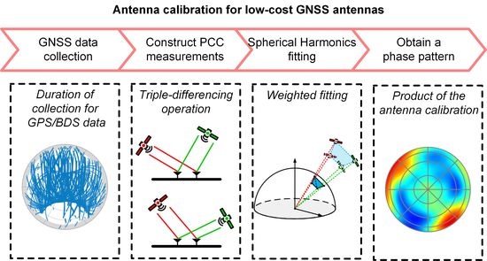
A Relative Field Antenna Calibration Method Designed for Low-Cost GNSS Antennas by Exploiting Triple-Differenced Measurements

1
School of Electronic and Information Engineering, Beijing Jiaotong University, Beijing 100044, China
2
College of Fashion Art and Engineering, Beijing Institute of Fashion Technology, Beijing 100029, China
*
Author to whom correspondence should be addressed.
Remote Sens. 2023, 15(15), 3917; https://doi.org/10.3390/rs15153917
Submission received: 22 May 2023
/
Revised: 2 August 2023
/
Accepted: 4 August 2023
/
Published: 7 August 2023
(This article belongs to the Special Issue Satellite Navigation and Signal Processing)
Abstract
:Performing the high-precision Global Navigation Satellite System (GNSS) applications with low-cost antennas is an up-and-coming research field. However, the antenna-induced phase biases, i.e., phase center corrections (PCCs), of the low-cost antennas can be up to centimeters and need to be calibrated in advance. The relative field antenna calibration method is easy to conduct, but the classical procedure entails integer ambiguity resolution, which may face the problem of low success rate under the centimeter-level PCCs. In this contribution, we designed a relative field calibration method suitable for the low-cost GNSS antennas. The triple-differencing operations were utilized to eliminate the carrier-phase ambiguities and then construct PCC measurements; the time-differencing interval was set to a relatively long time span, such as one hour, and the reference satellite was selected according to the angular distance it passed over during a time-differencing interval. To reduce the effect of significant triple-differencing noise, a weight setting method based on the area of a spherical quadrilateral was proposed for the spherical harmonics fitting process. The duration of the data collection with respect to GPS and BDS was discussed. The performance of the proposed method was assessed with real GPS and BDS observations and a variety of simulated phase patterns, showing that calibration results could be obtained with millimeter-level accuracy. The impact of cycle slip and elevation mask angle on the calibration results was also analyzed.
1. Introduction
The receiver antenna, as a key device in the Global Navigation Satellite System (GNSS) applications, can introduce biases into the carrier-phase observations. Such phase biases, also known as phase center corrections (PCC), cannot be neglected for high-precision positioning, and therefore, antenna calibration is an essential research field in GNSS. Most of the existing antenna calibration methods are widely used to calibrate high-grade antennas such as geodetic antennas but are not well suited for low-cost antennas such as patch antennas. The large-scale application of the low-cost antennas requires that the antenna calibration method shall be easy to conduct, and in addition, centimeter-level PCCs can degrade the success rate of integer ambiguity resolution during a classical antenna calibration process. To address these problems, this paper proposes a relative field antenna calibration method specifically designed for the low-cost GNSS antennas.
Anechoic chamber measurement is a method to accurately measure various characteristics of antennas. It measures an antenna in a room with few reflected signals, which can be considered an ideal environment. Mechanical instruments are used to control the rotation and tilt of the antenna under test and to measure the phase delay experienced by the signal as it is incident from different directions to the antenna [1]. The anechoic chamber measurement method enables the antenna calibrations to be performed under near-ideal conditions, but the cost of the chamber construction and other equipment is high. Another disadvantage of this method is that the use of non-real satellite signals during the calibration process may introduce some deviations into the calibration results [2,3].
Absolute field calibration methods collect real GNSS observations in a field environment using a reference antenna and an antenna under test simultaneously [4,5,6,7,8]. By using a specialized calibration robot that can keep an antenna in a constant position while changing its attitude, operators are able to orient the zenith of the antenna to a particular satellite in the sky at any moment following a designed calibration strategy. The benefits of the absolute field calibrations are as follows: (1) by continuously changing the attitude of the antenna under test, observations that fully cover the antenna hemisphere can be rapidly (about 4–6 h) collected, which is much faster than the relative field calibration method as will be mentioned later; (2) the entire antenna hemisphere, including the low-elevation regions, can be calibrated; and (3) the calibration results of the antenna under test are less dependent on the PCCs of the reference antenna since in a short time span, the direction of a selected satellite is almost constant with respect to the reference antenna, while the satellite signal is projected into the antenna under test from diverse angles [9]. Sutyagin and Tatarnikov [9] pointed out that the results of absolute field calibration are primarily affected by near-field multipath. Wübbena et al. [5] and Bilich and Mader [6] carried out a differencing operation on single- or double-differenced observations between two consecutive mean sidereal days, which can eliminate multipath errors and errors related to geometric distances; this method requires two data collections of hours on two consecutive days, during which the attitude of the antenna under test changes according to the same strategy but using a different initial attitude. Hu et al. [10] and Willi et al. [11] employed an epoch-wise approach, i.e., performing time difference with double-differenced observations at two epochs spaced several seconds apart; this epoch-wise approach can avoid the changing meteorological conditions over the span of two days. It should be noted that since the rotation of the antenna under test also introduces changes in the carrier-phase observations, the carrier-phase ambiguities cannot be eliminated by time-differencing operations. As with the anechoic chamber measurements, absolute field calibrations cannot be easily performed on a large scale.
Before the introduction of the absolute field calibration method, the relative field calibration method was widely used for antenna calibration [12,13,14]. Compared with the absolute field calibrations, in the relative field calibrations, both the reference antenna and antenna under test are stationary, and collected signals may be incident from low-elevation directions, so a more open test field and some measures for suppressing the reflected signals from the ground are required [15]. Another distinct disadvantage is that since the coverage of the measurements in the antenna hemisphere depends on the distribution of the satellite trajectory, there is no measurement in some directions, namely, the north hole or the south hole. A compromise is to calibrate only the elevation-dependent phase center variations (PCVs) [12,13,15]. There are, however, some other studies increasing the coverage of observations in the antenna hemisphere by collecting observations for two or more sessions and horizontally rotating the antenna under test at the beginning of each session, thus enabling the acquisition of elevation- and azimuth-dependent PCVs with the relative field calibration [16]. It should be noted that the relative field calibration result of the antenna under test is relative to the reference antenna. Early researchers usually used a specific type of antenna (AOAD/M_T) as the reference antenna and assumed that the reference antenna was ideal [12,13]. With the development of various antenna calibration techniques, subsequent studies often used an absolutely calibrated antenna as the reference antenna and then transformed the relative calibration results to absolute calibration results. Krietemeyer et al. [17] used double-difference residuals to derive between-antenna single-difference residuals, which were used as measurements for antenna calibration. However, the prerequisite for this method to hold is that the antenna-induced phase bias obeys the Gaussian distribution with zero mean, and as this premise may not be true for low-cost antennas with centimeter-level PCCs, this method is not applicable to our research. In addition, there are also commercial softwares available for relative field calibration, such as Bernese GNSS software 5.2 [15,16]. Overall, the relative field calibration is easy to implement, although it takes longer and is susceptible to interference.
The International GNSS Service (IGS) maintains a widely used antenna calibration product. And it contains a variety of type-mean calibration results, which are the average of the calibration results of more than four antennas of the same specified type. As Dawidowicz et al. [2] and Zhou et al. [18] have shown that for geodetic antennas used in permanent stations, there is only a difference of a few millimeters (mm) between the calibration results of antennas of the same type, the type-mean calibration results can be applied to eliminate most antenna-induced phase biases for high-grade antennas. However, for more widely used low-cost antennas, the difference between the antenna of same type is larger [19]; therefore, the low-cost antennas need individual calibrations. Since only a few institutions can perform the anechoic chamber antenna measurement, and even fewer can conduct the absolute field calibration [3,20], the relative field calibration is an attractive choice to perform individual antenna calibrations on a large scale.
Compared with geodetic antennas, the low-cost antennas hold larger PCCs, possibly up to centimeters (cm) [19], and most low-cost antennas are single-frequency; these characteristics can weaken the GNSS model and consequently affect the success rate of integer ambiguity resolution, which is usually an essential step in classical relative field antenna calibration approaches. To address this problem, we can either improve the performance of ambiguity resolution or simply avoid the ambiguity resolution procedure. For the former option, a multi-epoch manner such as a Kalman filter-based approach can be adopted, and the constraints such as a priori antenna coordinates can also be utilized to enhance the strength of the GNSS model, thereby improving the success rate of ambiguity resolution, but the unknown large PCCs might be absorbed in the ambiguity parameters; therefore, more work is needed to detect the subsequent incorrect solutions among the accepted ambiguity solutions. In contrast, the latter approach may be more efficient, where we can directly eliminate the ambiguities by triple difference after a cycle slip detection, thus avoiding the complicated ambiguity resolution process. In this research, we used the latter method and designed an antenna calibration method specifically for the low-cost GNSS antennas. Our contributions can be summarized as follows:
- We present an approach to construct PCC measurements with triple-differencing operations between two involved antennas, two satellites, and two epochs with a relatively long interval such as one hour. The reference satellite was selected by comparing the angular distance it passed across the sky during a time-differencing interval. The time-differencing operation bore the task of eliminating carrier-phase ambiguities, which meant that a cycle slip detection procedure was necessary.
- We propose a weight setting method for the spherical harmonic fitting of phase patterns. The weights were set according to the area of a spherical quadrilateral enclosed by the terminal points of four unit vectors, the PCCs on whose directions were the components of the PCC measurements.
- We discuss the appropriate durations of data collection for the Global Positioning System (GPS) and the BeiDou Navigation Satellite System (BDS). For a relative field calibration method, since the antennas involved were static, the duration of the data collection was determined by the distributions and the ground trace repeat period of satellites.
- We evaluated the performance of the proposed antenna calibration method using real GPS and BDS observations and a set of simulated phase patterns. Moreover, we discuss the test results in terms of the cycle slip, weighting, and elevation mask angle.
In the following, first, based on the model of antenna-induced phase bias, a new antenna calibration method is introduced. Next, test results are presented, and the performance of the proposed method is analyzed. After that, some related factors are discussed. Finally, a conclusion is given.
2. Materials and Methods
In this section, we first briefly describe the antenna-induced phase bias model and then present a new antenna calibration method, which was specifically designed for the low-cost antennas with centimeter-level PCCs.
In general, an antenna calibration process consists of two steps: data collection and phase pattern fitting. The purpose of data collection is to collect measurements of PCCs or PCC combinations, where other components contained in the carrier-phase observations have been resolved or eliminated as much as possible. The purpose of phase pattern fitting is to fit a PCC model with a set of functions like spherical harmonics and then derive the PCC values at the grid points on antenna hemisphere.
In the following, Section 2.2 concentrates on the data collection process, introducing a PCC measurements construction procedure based on triple-difference; Section 2.3 concerns the phase pattern fitting process, proposing a weight setting method based on the area of a spherical quadrilateral; and Section 2.4 investigates the duration of data collection with respect to GPS and BDS.
2.1. Model of Antenna-Induced Phase Bias
It is determined by the nature of the antenna that the signals incident from different directions suffer from different phase biases. Specifically, the antenna-induced phase bias refers to the distance between the antenna phase center (APC) and the antenna reference point (ARP) [19]. The APC is not fixed, and its position depends on the incident direction and carrier frequency of signal. The antenna-induced phase bias can be considered to consist of two components, namely, the phase center offset (PCO) and the phase center variation (PCV). The PCO, which is the distance between the ARP and an arbitrarily selected mean phase center, is introduced to be able to be used alone and eliminate most phase biases [12]. However, some research has also used a unified term, namely, the phase center correction (PCC), to denote the antenna-induced phase bias [2,11]. The relationship between the PCC, PCO, and PCV can be expressed as
where denotes the PCC, i.e., the antenna-induced phase bias; denotes the unit line-of-sight (LOS) vector from receiver to satellite; and and denote the azimuth and elevation of satellite, respectively. depends on the incident direction and carrier frequency of signal. The incident direction can be represented by and , while the frequency is dropped in this equation to improve conciseness since we concentrate on the single-frequency antennas in this contribution.
The antenna-induced phase bias is a major obstacle to the use of low-cost antennas for high-precision applications. In applications that utilize the precise carrier-phase observations, antenna-induced phase biases need to be eliminated by applying a predetermined antenna phase pattern, which can describe the distribution of antenna-induced phase biases in an antenna frame [21]. The process of determine the antenna phase pattern is called antenna calibration.
In field calibration approaches, there are always two antennas collecting GNSS observations: one reference antenna and one antenna under test, denoted as antennas 1 and 2, respectively. If the antenna-induced phase biases are not negligible, the carrier-phase observations of satellite s measured on the two antennas can be expressed as
where denotes the carrier-phase observation; subscripts 1 and 2 denote the index of the receiver antennas; superscript denotes the index of the satellite; denotes the distance from the phase center of the satellite transmitting antenna to that of the receiver antenna; denotes the carrier-phase wavelength; denotes the clock delay; denotes the speed of light; and denote the ionosphere delay and troposphere delay, respectively; denotes the carrier-phase ambiguity, which should be an integer; and ε denotes the measurement noise.
For the relative field calibration method, the baseline length is usually only a few meters, so the signals from a same satellite to the two antennas can be considered parallel. Furthermore, if the north reference points (NRPs) of both antennas keep pointing to the same direction, then the two incident directions would have the same azimuth and elevation in the frames of the two antennas, i.e., , . So, we can construct a relative phase pattern, i.e., differenced phase pattern between the antenna under test and the reference antenna, describing the relative PCCs between the two antennas. The between-antenna differenced carrier-phase measurements can be expressed as
where denotes the relative PCC, and the subscript 12 denotes the differencing operation between the antennas 1 and 2.
The relative phase pattern can be further converted to the absolute phase pattern if the phase pattern of the reference antenna is available or negligible. However, this would be unnecessary for some specific applications like dual-antenna heading determinations. In such cases, the carrier-phase observations are always used in differenced form, and the two antennas are relative static, so, the relative phase pattern can be applied directly to eliminate the antenna-induced phase biases. The relative phase pattern is what we pursue in this contribution. And in the following sections, we simply use the term phase pattern to denote the relative phase pattern.
2.2. Construction of PCC Measurements with Triple-Difference
For low-cost antennas, the PCCs can be up to centimeters, severely reducing the success rate of integer ambiguity resolution, which is incorporated in the classical double-differencing approach to eliminate ambiguities. To address this problem, we introduced a triple-differencing procedure. Figure 1 shows eight carrier-phase observations used to construct a triple-differenced PCC measurement. They were measured from two antennas 1 and 2, at two epochs and , where denotes the time-differencing interval. Each carrier-phase measurement could be expressed similar to (2), in which only was the GNSS observable that could be directly measured, and all other components except needed to be eliminated as much as possible.
The differencing operations between two antennas can eliminate most space-dependent errors like tropospheric and ionospheric delays; the satellite clock delay can also be eliminated. According to Equation (3), four relative PCC measurements can be constructed as
The receiver clock delay and other receiver-dependent errors can be further eliminated by between-satellite differencing operations. The four relative PCC measurements in Equation (4) can then be transformed to two between-antenna and between-satellite double-differenced PCC measurements, expressed as
where the superscript denotes the differencing operation between satellite and (r stands for “reference satellite”), and denotes the double-differenced PCC measurement.
The carrier-phase ambiguity can be eliminated by further time-differencing operation between two epochs, if both receivers continuously lock satellites over a time-differencing interval. The resulting triple-differenced PCC measurements can be expressed as
where denotes the time-differencing operation between epochs t and , and denotes the noise component, which is more significant than the double-differencing noise. The time-differencing interval should be long enough, ensuring the positions of the satellites change significantly. In this contribution, as the antenna under test was static, we used an empirical value of one hour.
Note that some research also adopted the time-differencing technique but with different purposes. Bilich and Mader [6] performed the time-difference over the time span of a mean sidereal day to eliminate the periodic multipath errors. Hu et al. [10] used an epoch-wise time-differencing manner to eliminate multipath errors, and the time-differencing interval was only several epochs. Hu et al. [10] also pointed out that a changing weather condition could disturb the periodicity of multipath error over a mean sidereal day, degrading the effect of time-differencing operation. In our contribution, the time-difference was utilized to eliminate the carrier-phase ambiguities.
The classical antenna calibration approaches usually adopt an integer ambiguity resolution procedure to estimate the carrier-phase ambiguities, while the low-cost GNSS antennas can cause some difficulties in ambiguity resolution. Table 1 shows that the success rate of ambiguity resolution can be affected in the centimeter-level phase bias and single-frequency case. From the last row of Table 1, we can also see that a multi-epoch method can achieve a relatively high ambiguity resolution success rate. However, since the size of the PCCs of low-cost antennas can be comparable with the carrier wavelength, PCCs might be absorbed in the ambiguities, resulting in incorrect solutions. In this work, we preferred to simply avoid the ambiguity resolution and directly eliminate the ambiguities with the time difference.
Consequently, we must deal with the cycle slip before the time-differencing operations. Cycle slip is an unpredictable but frequently encountered carrier-phase error that occurs when the receiver loses track of the number of the carrier-phase cycles [22,23,24,25]. There are two ways to cope with cycle slips: detection and correction. The cycle-slip correction is more complicated, time-consuming, and computationally intensive [26]. For triple-differenced measurements, even a small cycle slip can introduce a deviation comparable to wavelength, so we only detected and then rejected the observations with cycle slips. Since many low-cost antennas are single-frequency antennas, without loss of generality, we adopted three cycle-slip detection methods that only utilized single-frequency observations. Specifically, the first method we used was to detect cycle slips through the loss of lock indicator (LLI), which was provided by the receiver and available in the RINEX observation file [27] (p. 67). The LLI flag would be set if the receiver suffered from a loss of lock. The second method we adopted was the high-order phase differencing method; see [25]. The third method was to detect cycle slips by evaluating the triple-differencing residuals, which were obtained by differencing the double-differenced residuals at two adjacent epochs; if the time-differencing interval was shorter than one minute, the triple-differencing residual was normally at only the millimeter level [28,29]. Other cycle-slip detection methods could also be incorporated to achieve a more comprehensive detection.
In Equation (6), is a combination of geodetic distances between receiver and satellite antennas:
Each component can be calculated with the receiver positions, which were precisely predetermined, and satellite positions, which were calculated with GNSS orbit products provided by the Multi-GNSS Experiment (MGEX) of the International GNSS Service (IGS) [30]. The orbit products, also known as precise ephemeris, are available at the IGS website in the Standard Product 3 (SP3) format with a sampling of five minutes [31]. The precise ephemeris can be interpolated to derive the position of satellites at signal emitting time; see [32,33]. The accuracy of the orbit products is typically within a few centimeters, which can help improve the precision of the desired triple-differenced PCC measurements in Equation (6).
In the process of constructing the triple-differenced PCC measurements, we needed to ensure that each observation was used only once. And to better recover PCCs from the triple-differenced PCC measurements, the reference satellite needed to be properly selected. The further the distance between two points on the antenna hemisphere, the more likely it is that the difference between the corresponding PCCs will be greater. Therefore, among all satellites that have been continuously locked for epochs, it makes sense to set the reference satellite to the one with largest angular distance between its line-of-sight (LOS) vectors at epoch and epoch . The angular distance can be calculated by an inner product operation:
where denotes the unit LOS vector of satellite , expressed as
where denotes the satellite position derived from the precise ephemeris, and denotes the receiver antenna position that is measured in advance and keeps fixed during the data collection process.
The resulting set of triple-differenced PCC measurements can be expressed as
The flowchart of constructing the triple-differenced PCC measurements is summarized and depicted in Figure 2.
2.3. Weight Setting in Phase Pattern Fitting Process
The PCC measurements constructed using the triple-differencing approach contain greater noise compared with the double-differencing approach, especially under a long time-differencing interval. In order to reduce the impact of the triple-differencing noise on the accuracy of the subsequent phase pattern fitting result, it is necessary to design a weighting method, giving more weight to the PCC measurements that are more accurate. This section first briefly describes the unweighted phase pattern fitting procedure and then proposes a new weight setting method.
There are traditionally two approaches to model the elevation- and azimuth-dependent phase patterns: grid and spherical harmonics expansions [11,12]. Since the direction of the satellite LOS vectors fully covers the antenna hemisphere, the approach with spherical harmonics is more compelling and meaningful. Moreover, most recent studies adopt the spherical harmonics of degree of 8 or 12 [6,8,11,20,34].
Using the spherical harmonics expansion, the relative PCC measurements can be expressed as
where and denote the maximum degree and maximum order of spherical harmonics, denotes the normalized associated Legendre polynomial of degree n and order m, is a function of the sine of the elevation angle , and and denote the desired spherical harmonics coefficients that determine the phase pattern model. If we set and to 8 and 5, respectively, like the literature [6,34] showed, there will be 38 coefficients to be resolved.
The triple-differenced PCC measurement obtained in the last section is a combination of four relative PCCs:
By substituting Equation (11) into Equation (12), the triple-differenced PCC measurements can be expanded as a function of a set of azimuth and elevation angles:
Once the spherical harmonics coefficients are resolved, the PCC values at grid points can be derived from the fitted function. The common grid spacing used in the file igs14.atx is 5° [35].
The existing research usually sets a unitary weighting for all PCC measurements [6,9,11]. In the following, we present a weight setting method based on the area of spherical quadrilaterals.
Each triple-differenced PCC measurement is associated with four directions—the directions of the LOS vectors of satellites r and s at epochs and . As we can see from Figure 3, the terminal points of the four corresponding unit LOS vectors lie on the antenna unit hemisphere, and these points enclose a spherical quadrilateral ACBD. According to Equation (12), a triple-differenced PCC measurement contains two parts: (1) triple-differenced PCC and (2) the rest noise in triple-differenced carrier-phase observations. The magnitude of the second part is relatively stable once a reliable cycle-slip detection and rejection are completed, while the magnitude of the first part can fluctuate remarkably. The triple-differenced PCC reflects the differences between PCCs at four different directions. As the phase pattern of low-cost antennas are typically large in magnitude and asymmetrical in distribution, the more scattered the positions of involved PCCs are, the more likely a larger triple-differenced PCC is formed. Therefore, it is reasonable to give more weight to the PCC measurements that are formed by more scattered satellite directions.
In this contribution, we measured the degree of scatter with the area of the aforementioned spherical quadrilateral. The area of a spherical quadrilateral can be regarded as the sum of the areas of two spherical triangles. Among the aforementioned four points that lay on the unit antenna hemisphere, we first found out two points (denoted as A and B) that met the following criteria—the other two points (denoted as C and D) were distributed on either side of the great circle that passed through the two points A and B. This could be done by utilizing the geometric relations between the plane, which was determined by two points (A, B) and O (ARP), and the other two points (C, D). Then we could calculate the areas of the two spherical triangles, ΔABC and ΔABD.
According to the spherical trigonometry, the area of the spherical triangle ΔABC can be calculated by
where A, B, and C denote spherical angles, and denotes the radius of the antenna unit hemisphere.
According to the spherical law of cosines, three spherical angles can be calculated by
where , , and denote three sides of ΔABC. They are essentially three angular distances, and they can be calculated with the inner product of corresponding unit LOS vectors; see Equation (8).
The area of ΔABD can then be derived in the same way. Then we can obtain the area of the spherical quadrilateral ACBD, expressed as
Once the calculations for with respect to all triple-differenced PCC measurements are performed, the weighting matrix can be set to
where k denotes the indexes of triple-differenced PCC measurements. It should be noted that for a concave spherical quadrilateral, there can be two ways to select the points A and B, i.e., the common points of two spherical triangles. In that case, we choose the way that maximizes .
Moreover, in the proposed weight setting method, the factors like elevation and signal to noise ratio (SNR) were not considered, despite the fact that they are usually incorporated to form weightings in GNSS applications. Generally, the lower the elevation is, the lower SNR is, and the larger the measurement error included in the carrier-phase observations. It is also the low-elevation regions where multipath errors are more significant. To reduce these problems, we can set an elevation mask angle to reject the observations at low elevations. Consequently, the final fitted phase pattern would only cover the regions above the elevation mask angle.
2.4. Duration of Data Collection
For a relative field calibration approach, it is necessary to determine an appropriate data collection duration that is long enough to collect the required GNSS observations. The premise of a reliable antenna calibration is to collect GNSS observations that are distributed as densely and uniformly as possible over the antenna hemisphere [34]. However, since there were no attitude control robots in the relative field calibration setup, both antennas could only remain fixed or undergo a simple 180° horizontal rotation, waiting for the slow change of satellite distributions.
Most existing studies on the relative field calibration are related to GPS, which is a Medium Earth Orbit (MEO) constellation. A mean sidereal day is the duration taken for the Earth to rotate exactly 360°, which is about 23 h 56 min 4.1 s. For a static receiver antenna, the position of every GPS satellite is periodic with a period of a mean sidereal day [36] (pp. 12–19). So, we cannot densify the satellite distribution by extending the data collection duration to more than a mean sidereal day.
However, it is different for GNSS systems other than GPS. For example, due to a different design of the orbit altitude, the MEO satellites of BDS hold a ground trace repeat period of seven mean sidereal days [37]. We can see from Figure 4 that the trajectory of a BDS MEO satellite does not repeat within seven consecutive days. This can be exploited to improve the satellite distribution by continuously collecting data for seven days. Furthermore, because the construction of the third phase of BDS was not completed until 2020, many off-the-shelf receivers may not be able to capture all BDS satellites signals, making it much more valuable to extend the duration of data collection in a relative field antenna calibration.
The north hole (or south hole) also affects the satellite distribution, resulting in a region of sky with no visible satellites. A widely used method is to arrange two data collection sessions, between which the antenna under test is horizontally rotated 180° [16]. In our contribution, however, both antennas are supposed to be rotated, since we tend to obtain a relative phase pattern. Consequently, the GPS data could be collected for up to two days, with a horizontal rotation for both antennas at the beginning of the second day; the BDS data could be collected for up to 14 days, with a horizontal rotation for both antennas at the beginning of the eighth day.
3. Results
In this section, we evaluate the feasibility and performance of the proposed antenna calibration method. We adopt real GNSS observations collected with high-grade antennas and then artificially add simulated PCCs to the original observations to simulate the cases of low-cost antennas. The advantage of using simulated PCCs is that we can accurately evaluate the accuracy of the calibration results by comparing them with the phase patterns used to simulate the PCCs. In addition, we can flexibly test a variety of different phase patterns.
3.1. Data Preparation
We chose the data collected from two stations, CUTB and CUTC, at Curtin University. As for GPS, we selected two days, 30 April and 1 May 2022, and for BDS, we selected eight days, 30 April to 7 May 2022. The raw data were with a sample rate of 1 Hz, which was helpful to improve the reliability of cycle slip detections. Recall that the relative field antenna calibration is challenged by the south hole (at the southern hemisphere). To simulate a data collection session where both antennas were horizontally rotated 180°, we transformed the azimuths of all satellites on the first day, 30 April 2022, with 180° increments. Therefore, the two data collection sessions for GSP were both one day, while the two sessions for BDS were one and seven days, respectively.
The top panel of Figure 5 depicts the number of common-view satellites. Note that since we adopted the precise ephemeris to calculate the positions of satellites, the satellites without an available precise ephemeris were not counted, such as GPS satellite PRN 11. Furthermore, we note that the receivers could only record the observations of BDS satellites of PRN smaller than 30, while the full constellation of BDS consists of 44 satellites. This may have been due to the receivers not yet being updated to be capable of receiving all BDS satellites, as the BDS had not achieved a full constellation until the end of 2020.
The bottom panel of Figure 5 shows the number of triple-differenced PCC measurements we constructed. As the blue shadows indicate, in the two time periods at the first and third days, the number of PCC measurements was low due to the small number of common-view satellites. However, there were also cases where the number of constructed PCC measurements was low during the period when the number of common-view satellites did not decrease. For example, on the eighth day, the number of constructed PCC measurements for BDS never exceeded six. This could be due to the cycle slip; we will come back to this later.
In addition to the number of PCC measurements, the coverage of the satellites that are involved in constructing the PCC measurements are also important to the phase pattern fitting. To illustrate the distribution of these satellites, we provide the skyplots of GPS and BDS satellites in two and eight consecutive days, respectively, in Figure 6. Note that we artificially added 180° to the azimuth of satellites on the first day, filling the south hole. The distribution of GPS satellites was denser in the high-elevation region, compared with the north and south regions. We can also see that the distribution of BDS satellites was denser, as the data collection lasted longer.
Specifically, since the second session of data collection for BDS lasted for seven days, the north region in Figure 6b was as dense as the high-elevation region. Remark that this benefited from the fact that the ground trace repeat period of BDS MEO satellites was seven mean sidereal days. From Figure 7, we can also see that the satellite distribution of BDS kept changing during seven consecutive days. Consequently, although there were fewer observations available for constructing PCC measurements on the third (Figure 7b) and eighth days (Figure 7g), the overall satellite coverage was still good. Therefore, if sufficient time is available, it is recommended to collect the BDS data for up to 14 days, i.e., two sessions lasting for seven days each.
As we have stated, we artificially added simulated PCCs to the original precise carrier-phase observations to simulate the cases of low-cost antennas. To sufficiently test the performance of the proposed antenna calibration method, we constructed eight random phase patterns, as shown in Figure 8, and they were labeled from a to h. Their magnitudes are at the centimeter level but less than half of the GPS L1 wavelength. It should be noted that in the following tests, they were artificially added to the carrier-phase observations of both GPS L1 and BDS B1 signals, so that we could compare the performances of the proposed antenna calibration method under different navigation systems.
3.2. GPS Antenna Calibration Results
In this section, the antenna calibration results for GPS are illustrated. The elevation mask angle was set to 0° so that all available observations were utilized to construct the PCC measurements and then fit the phase pattern. Figure 9 shows the GPS antenna calibration results, i.e., the fitted phase patterns. Compared with the reference phase pattern shown in Figure 8, we can see that the shapes of the fitted phase pattern were consistent with the reference. And the most obvious difference was the larger magnitude of the calibration results.
To better demonstrate the accuracy of the calibration results, we depict the distributions of the phase pattern fitting deviations in Figure 10. We can see that in the regions where the elevation angles were higher than 10°, the deviations were at the millimeter level. However, in the regions where the elevation angles were lower than 10°, the phase pattern fitting deviations could reach up to several centimeters. Table 2 summarizes the statistics of the calibration deviations. It shows that the root mean square errors (RMSEs) of all eight calibration results were at the mm level, but the maximum deviation was relatively large. Even the best calibration result, (a), held a maximum deviation of 19 mm. A reasonable explanation is that there were more frequent cycle slips at low elevation angles, resulting in only a few available observations. This can be validated by Figure 6a, from which we can see that at elevation angles lower than 10° (indicated by the gray shadow), the distribution of available satellites was extremely sparse.
3.3. BDS Antenna Calibration Results
In this section, we show the antenna calibration results for BDS. The elevation mask angle was set to 0°. The most significant features of the BDS data were a longer data collection duration and denser satellite distribution (as shown in Figure 6). Therefore, a better calibration result than GPS could be expected.
Figure 11 depicts the BDS antenna calibration results, which were more comparable to the reference phase pattern, compared with the GPS calibration results. Figure 12 shows the deviation distributions of each calibration result. For better comparison, we use a uniform color map with Figure 10. It can be seen that only some small areas below the elevation angle of 10° suffered from deviations larger than 1 cm, and the maximum deviation was lower than 2 cm. Table 3 summarizes the statistics of the BDS calibration deviations. The mean value of eight RMSEs was 3.378 mm, which was about half that of the GPS calibration results. This is mainly due to more available BDS observations, which improves the calibration results at low elevation angles.
4. Discussion
In this section, we discuss the test results, as well as analyze some factors that can affect the performance of the proposed antenna calibration method.
4.1. Cycle Slip
In our triple-differencing approach, the availability of GNSS observations, and therefore the number of constructed PCC measurements, are susceptible to cycle slips since the carrier-phase ambiguities are to be eliminated by the time-differencing operation. Figure 13 shows the numbers of detected cycle-slips. It is obvious that at the eighth day, there were a remarkably large number of cycle-slips. This explains why only a small number of PCC measurements were obtained on the eighth day, while the number of common-view satellites was normal. Both Figure 5 and Figure 7g have already illustrated this. In addition to the eighth day, the other days also suffered from a considerable number of cycle slips. Specifically, the average numbers of cycle slips in one minute were 24.53 and 61.49 for GPS and BDS, respectively. The quantity as well as the frequency of cycle slip can severely reduce the number of available GNSS observations. For example, if the time-differencing interval is set to one hour, and a satellite suffers from a cycle-slip every 50 min, then all the observations of this satellite cannot be used to construct the triple-differenced PCC measurements.
Furthermore, when the low-cost GNSS antennas are adopted, the cycle slips can be even more severe. In our tests, we used a combination of real GNSS observations and simulated PCCs to construct the test data, where the original GNSS observations were collected by high-grade antennas. Compared with the high-grade antennas, the low-cost antennas have difficulty suppressing multipath interference, and the output signal strength is relatively weak, all of which can cause cycle slips.
Consequently, some compensation methods are needed to cease cycle slips during the data collection process: (1) collect data using high-quality GNSS receivers with stabilized clocks, and choose the cables with good low-loss characteristics; (2) carefully select the data collection site, and keep the surrounding area clear of objects that may block satellite signals, therefore reducing the case of signal interruption; and (3) adopt appropriate methods, such as installing a choke ring, to suppress signals of the negative elevation angle. Considering that the antennas are static during the data collection process, the above method should be able to relieve frequent cycle slips. Moreover, under harsher cases, it is possible to increase the number of constructed PCC measurements by extending the data collection duration by a few days, or decreasing the time-differencing interval as long as it can be guaranteed that there is a significant change of satellite distribution over the interval.
4.2. Weighting
In Section 2.3, we presented a weight setting method based on the area of a spherical quadrilateral enclosed by four terminal points of unit vectors. For an inhomogeneous phase pattern, the further apart two directions are, the more likely the corresponding PCCs are to be significantly different. Our method used triple-differenced PCC measurements, i.e., a combination of the relative PCCs at four different directions. Consequently, the more scattered the four directions are, the more likely the value of triple-differenced PCC are to be larger. Note that the triple-differenced PCC differs from the triple-differenced PCC measurement, where the former includes only the differences between PCC values, while the latter also includes the rest noise in the triple-differenced observations.
Figure 14 depicts the relationship between the size of the triple-differenced PCCs and the corresponding weightings. From the slopes of the fitted lines, we can see that in most cases (13 out of 16), the sizes of the triple-differenced PCCs were directly proportional to the weights. It therefore makes sense to use the area of a spherical quadrilateral to weight the spherical harmonics fitting. It should also be noted that according to the values of the coefficients of determination (R2), there was a considerable amount of triple-differenced PCC data that did not correspond to the fitted linear function, especially for the GPS case. As the tests for GPS and BDS used the same set of phase patterns, the differences in R2 between GPS and BDS should be due to the fact that the coverage of the collected GPS observations was sparser. The low values of R2 are reasonable because the values of the PCC in two directions far apart may also be very similar, i.e., when the area of the spherical quadrilateral is large, the value of triple-differenced PCC can also be potentially small.
However, the value of the PCC is a continuous variable in the antenna hemisphere, so when the four directions are quite close, the value of triple-differenced PCC is very small. In this case, the accuracy of the triple-differenced PCC measurements will be severely affected by the rest noise in the triple-differenced observations. During the phase pattern fitting process, setting the weights according to the area of the spherical quadrilateral can relieve the above problem, thus reducing the impact of the triple-differenced noise as much as possible. In addition, the proposed weight setting method also helps to better characterize the phase pattern at larger scales in the phase pattern fitting results.
4.3. Elevation Mask Angle
As we have seen from Figure 10, the calibration results could be degraded as there were almost no observations available at low-elevation regions. Therefore, an appropriate elevation mask angle may be helpful to improve the calibration results. We test three elevation mask angle settings—0°, 10°, and 20°—and the RMSEs of the corresponding results for GPS and BDS are listed in Table 4 and Table 5, respectively. On one hand, under the setting of 0°, the average RMSE for the antenna calibration results with GPS was 2.15 times that with BDS. Then it decreased to 1.41 and 1.45 times under the settings of 10° and 20°, respectively. This indicates that the disadvantage of lack of GPS data at low elevation region is erased. The remaining gap can be attributed to the shorter duration of GPS data collection. Meanwhile, however, it is reasonable to expect that the BDS results could be further improved by extending the first data collection session and filling the south hole with more available observations. On the other hand, within the calibration results of either GPS or BDS, there was a clear trend toward decreasing RMSE as the elevation mask angle increased. This is in line with the larger number of available observations in the high-elevation regions, which we have seen in Figure 6. In conclusion, before the phase pattern fitting process, we can evaluate the distribution of available observations and then set an appropriate elevation mask angle—if there are hardly any available observations below a certain elevation angle, we can set the elevation mask angle to that value. The consequent fitted phase pattern might have a smaller coverage, but its accuracy can be improved.
5. Conclusions
We specifically designed a relative field antenna calibration method for low-cost GNSS antennas, whose PCC can be up to several centimeters. By employing the triple-differencing operation, we constructed a set of PCC measurements, which could be considered as a combination of relative PCC values at four different directions. The carrier-phase ambiguities were eliminated by the time-differencing operations. The time-differencing interval was set to a relatively long period such as one hour. The reference satellite in the between-satellite difference was selected according to the angular distance it passed over during the time-differencing interval. As for the phase pattern fitting process, we presented a weight setting method based on the area of a spherical quadrilateral, which was enclosed by the terminal points of four unit LOS vectors, the PCCs on whose directions were the components of the corresponding PCC measurements. The appropriate data collection duration was discussed with respect to GPS and BDS. The performance of the proposed method was evaluated with real GPS and BDS observations and eight simulated phase patterns, indicating that a calibration result with a mm-level RMSE could be obtained. The impact of cycle slip and elevation mask angle was also discussed, showing that a longer data collection duration and an appropriate elevation mask angle could be set under challenging conditions. Since the data collected from the low-cost GNSS antennas are more complicated than those collected from the high-grade antennas, such as lower signal strength and more cycle slips, an essential future work is to conduct field experiments with a variety of low-cost GNSS antennas in order to sufficiently validate the proposed antenna calibration method. Despite this vacuum, we hope that this work can still bring some insight to the antenna calibrations for low-cost antennas. Moreover, our proposed weight setting method only concerned the scatter of the unit LOS vectors; a conceivable direction for future work is to incorporate the elevation angle and the SNR into the weighting.
Author Contributions
Conceptualization and methodology, W.J., W.G. and T.H.; software, data curation, and validation, W.J. and W.G.; writing—original draft preparation, W.J. and T.H.; writing—review and editing, W.G., T.H., X.S. and H.M.; supervision, W.G. and X.S.; funding acquisition, T.H. and X.S. All authors have read and agreed to the published version of the manuscript.
Funding
This research was funded by the Young Elite Scientists Sponsorship Program by CAST, grant number 2022QNRC001, and the National Natural Science Foundation for Young Scientists of China, grant number 62201028.
Data Availability Statement
The GNSS observation data can be found on the website of the GNSS Research Center at Curtin University (http://saegnss2.curtin.edu/ldc/rawdata/2022/ (accessed on 17 April 2023)). The precise ephemeris data can be found on the website of the IGS data center of Wuhan University (ftp://igs.ign.fr/pub/igs/products/mgex/2208/ (accessed on 17 April 2023)). The other data used in this manuscript are available from the corresponding author upon request.
Acknowledgments
We would like to express our gratitude to the academic editor and anonymous reviewers for their constructive comments and suggestions. We thank GNSS Research Center of Curtin University and the IGS data center of Wuhan University for providing GNSS data.
Conflicts of Interest
The authors declare no conflict of interest.
References
- Schupler, B.R.; Allshouse, R.L.; Clark, T.A. Signal Characteristics of GPS User Antennas. Navigation 1994, 41, 276–296. [Google Scholar] [CrossRef]
- Dawidowicz, K.; Krzan, G.; Wielgosz, P. Offsets in the EPN station position time series resulting from antenna/radome changes: PCC type-dependent model analyses. GPS Solut. 2022, 27, 9. [Google Scholar] [CrossRef]
- Dawidowicz, K. Impact of different GNSS antenna calibration models on height determination in the ASG-EUPOS network: A case study. Surv. Rev. 2013, 45, 386–394. [Google Scholar] [CrossRef]
- Wübbena, G.; Schmitz, M.; Menge, F.; Seeber, G.; Völksen, C. A New Approach for Field Calibration of Absolute GPS Antenna Phase Center Variations. Navigation 1997, 44, 247–255. [Google Scholar] [CrossRef]
- Wübbena, G.; Schmitz, M.; Menge, F.; Böder, V.; Seeber, G. Automated Absolute Field Calibration of GPS Antennas in Real-Time. In Proceedings of the 13th International Technical Meeting of the Satellite Division of the Institute of Navigation (ION GPS 2000), Salt Lake City, UT, USA, 19–22 September 2000; pp. 2512–2522. [Google Scholar]
- Bilich, A.; Mader, G.L. GNSS absolute antenna calibration at the national geodetic survey. In Proceedings of the 23rd International Technical Meeting of the Satellite Division of the Institute of Navigation (ION GNSS 2010), Portland, OR, USA, 21–24 September 2010; pp. 1369–1377. [Google Scholar]
- Görres, B.; Campbell, J.; Becker, M.; Siemes, M. Absolute calibration of GPS antennas: Laboratory results and comparison with field and robot techniques. GPS Solut. 2006, 10, 136–145. [Google Scholar] [CrossRef]
- Kröger, J.; Kersten, T.; Breva, Y.; Schön, S. Multi-frequency multi-GNSS receiver antenna calibration at IfE: Concept-calibration results-validation. Adv. Space Res. 2021, 68, 4932–4947. [Google Scholar] [CrossRef]
- Sutyagin, I.; Tatarnikov, D. Absolute robotic GNSS antenna calibrations in open field environment. GPS Solut. 2020, 24, 92. [Google Scholar] [CrossRef]
- Hu, Z.; Zhao, Q.; Chen, G.; Wang, G.; Dai, Z.; Li, T. First Results of Field Absolute Calibration of the GPS Receiver Antenna at Wuhan University. Sensors 2015, 15, 28717–28731. [Google Scholar] [CrossRef] [Green Version]
- Willi, D.; Koch, D.; Meindl, M.; Rothacher, M. Absolute GNSS Antenna Phase Center Calibration with a Robot. In Proceedings of the 31st International Technical Meeting of the Satellite Division of the Institute of Navigation (ION GNSS+ 2018), Miami, FL, USA, 24–28 September 2018; pp. 3909–3926. [Google Scholar]
- Rothacher, M.; Schaer, S.; Mervart, L.; Beutler, G. Determination of antenna phase center variations using GPS data. In IGS Workshop Proceedings: Special Topics and New Directions; GeoForschungsZentrum: Potsdam, Germany, 1995; pp. 205–220. [Google Scholar]
- Mader, G.L. GPS Antenna Calibration at the National Geodetic Survey. GPS Solut. 1999, 3, 50–58. [Google Scholar] [CrossRef]
- Akrour, B.; Santerre, R.; Geiger, A. Calibrating antenna phase centers. GPS World 2005, 16, 49–53. [Google Scholar]
- Biagi, L.; Grec, F.-C.; Fermi, A.; Negretti, M. Relative Antenna Calibration for Mass-Market GNSS Receivers: A Case Study. 2018. Available online: https://www.researchgate.net/profile/Florin-Catalin-Grec/publication/328074695_Relative_antenna_calibration_for_mass-market_GNSS_receivers_A_case_study/links/5bb626184585153610ac0b53/Relative-antenna-calibration-for-mass-market-GNSS-receivers-A-case-study.pdf (accessed on 25 January 2023). [CrossRef]
- Willi, D.; Meindl, M.; Xu, H.; Rothacher, M. GNSS antenna phase center variation calibration for attitude determination on short baselines. Navigation 2018, 65, 643–654. [Google Scholar] [CrossRef]
- Krietemeyer, A.; Van Der Marel, H.; Van De Giesen, N.; Ten Veldhuis, M.-C. A Field Calibration Solution to Achieve High-Grade-Level Performance for Low-Cost Dual-Frequency GNSS Receiver and Antennas. Sensors 2022, 22, 2267. [Google Scholar] [CrossRef] [PubMed]
- Zhou, R.; Hu, Z.; Zhao, Q.; Cai, H.; Liu, X.; Liu, C.; Wang, G.; Kan, H.; Chen, L. Consistency Analysis of the GNSS Antenna Phase Center Correction Models. Remote Sens. 2022, 14, 540. [Google Scholar] [CrossRef]
- Rao, B.R.; Kunysz, W.; Fante, R.; McDonald, K. GPS/GNSS Antennas; Artech House: London, UK, 2013. [Google Scholar]
- Willi, D.; Lutz, S.; Brockmann, E.; Rothacher, M. Absolute field calibration for multi-GNSS receiver antennas at ETH Zurich. GPS Solut. 2019, 24, 28. [Google Scholar] [CrossRef]
- Leick, A.; Rapoport, L.; Tatarnikov, D. GPS Satellite Surveying, 4th ed.; John Wiley & Sons: Hoboken, NJ, USA, 2015. [Google Scholar]
- Liu, Z. A new automated cycle slip detection and repair method for a single dual-frequency GPS receiver. J. Geodesy 2011, 85, 171–183. [Google Scholar] [CrossRef]
- Cai, C.; Liu, Z.; Xia, P.; Dai, W. Cycle slip detection and repair for undifferenced GPS observations under high ionospheric activity. GPS Solut. 2013, 17, 247–260. [Google Scholar] [CrossRef]
- Zhang, X.; Li, P. Benefits of the third frequency signal on cycle slip correction. GPS Solut. 2016, 20, 451–460. [Google Scholar] [CrossRef]
- Dai, Z. MATLAB software for GPS cycle-slip processing. GPS Solut. 2012, 16, 267–272. [Google Scholar] [CrossRef] [Green Version]
- Karaim, M.O.; Karamat, T.B.; Noureldin, A.; Tamazin, M.; Atia, M.M. Real-time Cycle-slip Detection and Correction for Land Vehicle Navigation using Inertial Aiding. In Proceedings of the 26th International Technical Meeting of the Satellite Division of The Institute of Navigation (ION GNSS+ 2013), Nashville, TN, USA, 16–20 September 2013. [Google Scholar]
- IGS RINEX WG RTCM-SC104. RINEX The Receiver Independent Exchange Format, Version 3.04. 2018. Available online: https://files.igs.org/pub/data/format/rinex304.pdf (accessed on 25 June 2023).
- Kim, D.; Langley, R.B. Instantaneous Real-Time Cycle-Slip Correction for Quality Control of GPS Carrier-Phase Measurements. Navigation 2002, 49, 205–222. [Google Scholar] [CrossRef]
- Wang, B.; Miao, L.; Wang, S.; Shen, J. An integer ambiguity resolution method for the global positioning system (GPS)-based land vehicle attitude determination. Meas. Sci. Technol. 2009, 20, 075108. [Google Scholar] [CrossRef]
- Montenbruck, O.; Steigenberger, P.; Prange, L.; Deng, Z.G.; Zhao, Q.L.; Perosanz, F.; Romero, I.; Noll, C.; Sturze, A.; Weber, G.; et al. The Multi-GNSS Experiment (MGEX) of the International GNSS Service (IGS)—Achievements, prospects and challenges. Adv. Space Res. 2017, 59, 1671–1697. [Google Scholar] [CrossRef]
- Hilla, S. The Extended Standard Product 3 Orbit Format (SP3-d). 2016. Available online: https://files.igs.org/pub/data/format/sp3d.pdf (accessed on 5 April 2023).
- Yousif, H.; El-Rabbany, A. Assessment of several interpolation methods for precise GPS orbit. J. Navig. 2007, 60, 443–455. [Google Scholar] [CrossRef]
- Song, C.; Chen, H.; Jiang, W.; An, X.; Chen, Q.; Li, W. An effective interpolation strategy for mitigating the day boundary discontinuities of precise GNSS orbit products. GPS Solut. 2021, 25, 99. [Google Scholar] [CrossRef]
- Dawidowicz, K.; Rapiński, J.; Śmieja, M.; Wielgosz, P.; Kwaśniak, D.; Jarmołowski, W.; Grzegory, T.; Tomaszewski, D.; Janicka, J.; Gołaszewski, P.; et al. Preliminary Results of an Astri/UWM EGNSS Receiver Antenna Calibration Facility. Sensors 2021, 21, 4639. [Google Scholar] [CrossRef]
- Rothacher, M.; Schmid, R. ANTEX: The Antenna Exchange Format, Version 1.4. 2010. Available online: https://files.igs.org/pub/station/general/antex14.txt (accessed on 5 May 2023).
- Van Diggelen, F. A-GPS: Assisted GPS, GNSS, and SBAS; Artech House: London, UK, 2009. [Google Scholar]
- Gao, W.; Meng, X.; Gao, C.; Pan, S.; Zhu, Z.; Xia, Y. Analysis of the carrier-phase multipath in GNSS triple-frequency observation combinations. Adv. Space Res. 2019, 63, 2735–2744. [Google Scholar] [CrossRef]
Figure 1.
Illustration of triple-difference between two epochs, between two satellites, and over a constant baseline (BL).
Figure 1.
Illustration of triple-difference between two epochs, between two satellites, and over a constant baseline (BL).

Figure 2.
Flowchart of constructing the triple-differenced PCC measurements.

Figure 3.
Illustration of the spherical quadrilateral ACBD enclosed by four terminal points of satellite unit LOS vectors. The solid and dashed satellite icons stand for the satellite positions at epochs and , respectively.
Figure 3.
Illustration of the spherical quadrilateral ACBD enclosed by four terminal points of satellite unit LOS vectors. The solid and dashed satellite icons stand for the satellite positions at epochs and , respectively.

Figure 4.
Skyplot of PRN 29 of BDS in seven consecutive days (1–7 May 2022) at Curtin.

Figure 5.
Number of common-view satellites (top) and constructed PCC measurements (bottom). The GPS data were collected for two days, and the BDS data were collected for eight days. The blue shadows denote the time periods where the number of common-view satellites was relatively low.
Figure 5.
Number of common-view satellites (top) and constructed PCC measurements (bottom). The GPS data were collected for two days, and the BDS data were collected for eight days. The blue shadows denote the time periods where the number of common-view satellites was relatively low.

Figure 6.
Skyplot of (a) the GPS and (b) the BDS satellites that were used to construct the PCC measurements. These data were collected for two and eight days, respectively.
Figure 6.
Skyplot of (a) the GPS and (b) the BDS satellites that were used to construct the PCC measurements. These data were collected for two and eight days, respectively.

Figure 7.
Skyplot of the BDS satellites that were used to construct the PCC measurements in the seven consecutive days (from (a–g) 1 to 7 May 2022).
Figure 7.
Skyplot of the BDS satellites that were used to construct the PCC measurements in the seven consecutive days (from (a–g) 1 to 7 May 2022).

Figure 8.
A set of simulated antenna phase patterns (a–h) different examples.

Figure 9.
GPS antenna calibration results (a–h) different examples.

Figure 10.
GPS antenna calibration deviations (a–h) different examples.

Figure 11.
BDS antenna calibration results (a–h) different examples.

Figure 12.
BDS antenna calibration deviations (a–h) different examples.
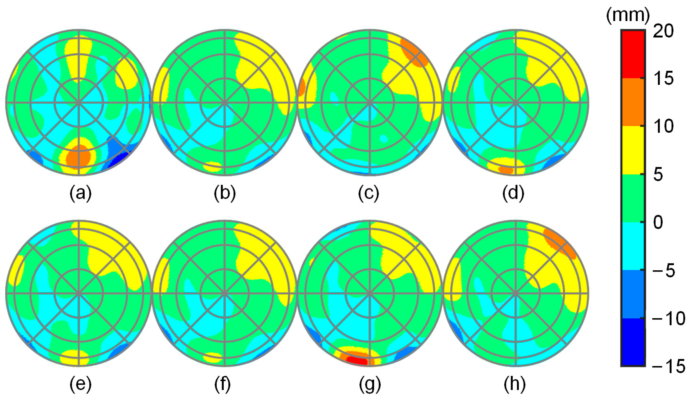
Figure 13.
Number of detected cycle-slips at each day.

Figure 14.
The relationship between triple-differenced PCCs and weightings. The bold black line plots the fitted linear function. In addition, the slope and the coefficient of determination (R2) of each fitted line are indicated above each subfigure. The unexpected cases, where the slope of the fitted linear function is negative, are marked in red.


Table 1.
Example of ambiguity resolution success rate (%) under different sizes of phase biases at a baseline of around 4 m. The sizes of the phase biases were random values within the specified intervals. The data of the multi-epoch case were derived using a Kalman filter-based method.
Table 1.
Example of ambiguity resolution success rate (%) under different sizes of phase biases at a baseline of around 4 m. The sizes of the phase biases were random values within the specified intervals. The data of the multi-epoch case were derived using a Kalman filter-based method.
| Size of Phase Bias (cm) | 0 | 0~1 | 0~2 | 0~3 | 0~4 | 0~5 | 0~6 |
|---|---|---|---|---|---|---|---|
| Single-frequency, single-epoch | 41.0 | 11.7 | 1.7 | 0.9 | 0.8 | 0.8 | 0.8 |
| Single-frequency, multi-epoch | 79.2 | 79.0 | 78.0 | 75.4 | 73.4 | 71.9 | 67.8 |
Table 2.
Statistics (root mean square error (RMSE), maximum deviation (Max.), and minimum deviation (Min.)) of GPS antenna calibration deviations.
Table 2.
Statistics (root mean square error (RMSE), maximum deviation (Max.), and minimum deviation (Min.)) of GPS antenna calibration deviations.
| Statistics | a | b | c | d | e | f | g | h |
|---|---|---|---|---|---|---|---|---|
| RMSE (mm) | 4.191 | 7.218 | 7.500 | 7.402 | 7.365 | 7.226 | 7.956 | 9.211 |
| Max. (mm) | 19.061 | 15.132 | 20.036 | 12.119 | 11.838 | 15.104 | 12.563 | 20.471 |
| Min. (mm) | −15.842 | −36.827 | −38.949 | −38.266 | −38.896 | −36.868 | −41.133 | −48.909 |
Table 3.
Statistics of BDS antenna calibration deviations.
| Statistics | a | b | c | d | e | f | g | h |
|---|---|---|---|---|---|---|---|---|
| RMSE (mm) | 3.547 | 3.149 | 3.566 | 3.174 | 3.084 | 3.149 | 3.587 | 3.767 |
| Max. (mm) | 14.884 | 9.434 | 13.328 | 10.997 | 9.351 | 9.422 | 17.973 | 12.432 |
| Min. (mm) | −14.934 | −7.666 | −7.445 | −9.066 | −9.438 | −7.678 | −9.651 | −8.764 |
Table 4.
RMSEs (mm) of GPS antenna calibration results with different elevation mask angle settings.
Table 4.
RMSEs (mm) of GPS antenna calibration results with different elevation mask angle settings.
| Elevation Mask Angle | a | b | C | d | e | f | g | h |
|---|---|---|---|---|---|---|---|---|
| 0° | 4.191 | 7.218 | 7.500 | 7.402 | 7.365 | 7.226 | 7.956 | 9.211 |
| 10° | 3.385 | 4.253 | 4.428 | 4.322 | 4.373 | 4.256 | 4.467 | 4.937 |
| 20° | 2.894 | 3.864 | 3.877 | 3.983 | 3.973 | 3.868 | 4.185 | 4.479 |
Table 5.
RMSEs (mm) of BDS antenna calibration results with different elevation mask angle settings.
Table 5.
RMSEs (mm) of BDS antenna calibration results with different elevation mask angle settings.
| Elevation Mask Angle | a | b | c | d | e | f | g | h |
|---|---|---|---|---|---|---|---|---|
| 0° | 3.547 | 3.149 | 3.566 | 3.174 | 3.084 | 3.149 | 3.587 | 3.767 |
| 10° | 3.348 | 2.888 | 3.110 | 2.881 | 2.807 | 2.888 | 3.122 | 3.433 |
| 20° | 3.114 | 2.531 | 2.707 | 2.477 | 2.440 | 2.531 | 2.601 | 3.056 |
Disclaimer/Publisher’s Note: The statements, opinions and data contained in all publications are solely those of the individual author(s) and contributor(s) and not of MDPI and/or the editor(s). MDPI and/or the editor(s) disclaim responsibility for any injury to people or property resulting from any ideas, methods, instructions or products referred to in the content. |
© 2023 by the authors. Licensee MDPI, Basel, Switzerland. This article is an open access article distributed under the terms and conditions of the Creative Commons Attribution (CC BY) license (https://creativecommons.org/licenses/by/4.0/).
Share and Cite
MDPI and ACS Style
Jin, W.; Gong, W.; Hou, T.; Sun, X.; Ma, H. A Relative Field Antenna Calibration Method Designed for Low-Cost GNSS Antennas by Exploiting Triple-Differenced Measurements. Remote Sens. 2023, 15, 3917. https://doi.org/10.3390/rs15153917
AMA Style
Jin W, Gong W, Hou T, Sun X, Ma H. A Relative Field Antenna Calibration Method Designed for Low-Cost GNSS Antennas by Exploiting Triple-Differenced Measurements. Remote Sensing. 2023; 15(15):3917. https://doi.org/10.3390/rs15153917
Chicago/Turabian StyleJin, Wenxin, Wenfei Gong, Tianwei Hou, Xin Sun, and Hao Ma. 2023. "A Relative Field Antenna Calibration Method Designed for Low-Cost GNSS Antennas by Exploiting Triple-Differenced Measurements" Remote Sensing 15, no. 15: 3917. https://doi.org/10.3390/rs15153917
Note that from the first issue of 2016, this journal uses article numbers instead of page numbers. See further details here.