
Validation of the Ocean Wave Spectrum from the Remote Sensing Data of the Chinese–French Oceanography Satellite
Abstract
:
1. Introduction
2. Materials and Methods
2.1. CFOSAT Data
2.2. In Situ Buoy Data
2.3. Validation Method
2.4. Filtering Method
2.5. Separating Method for Wind Wave and Swell
3. CFOSAT WS Validation
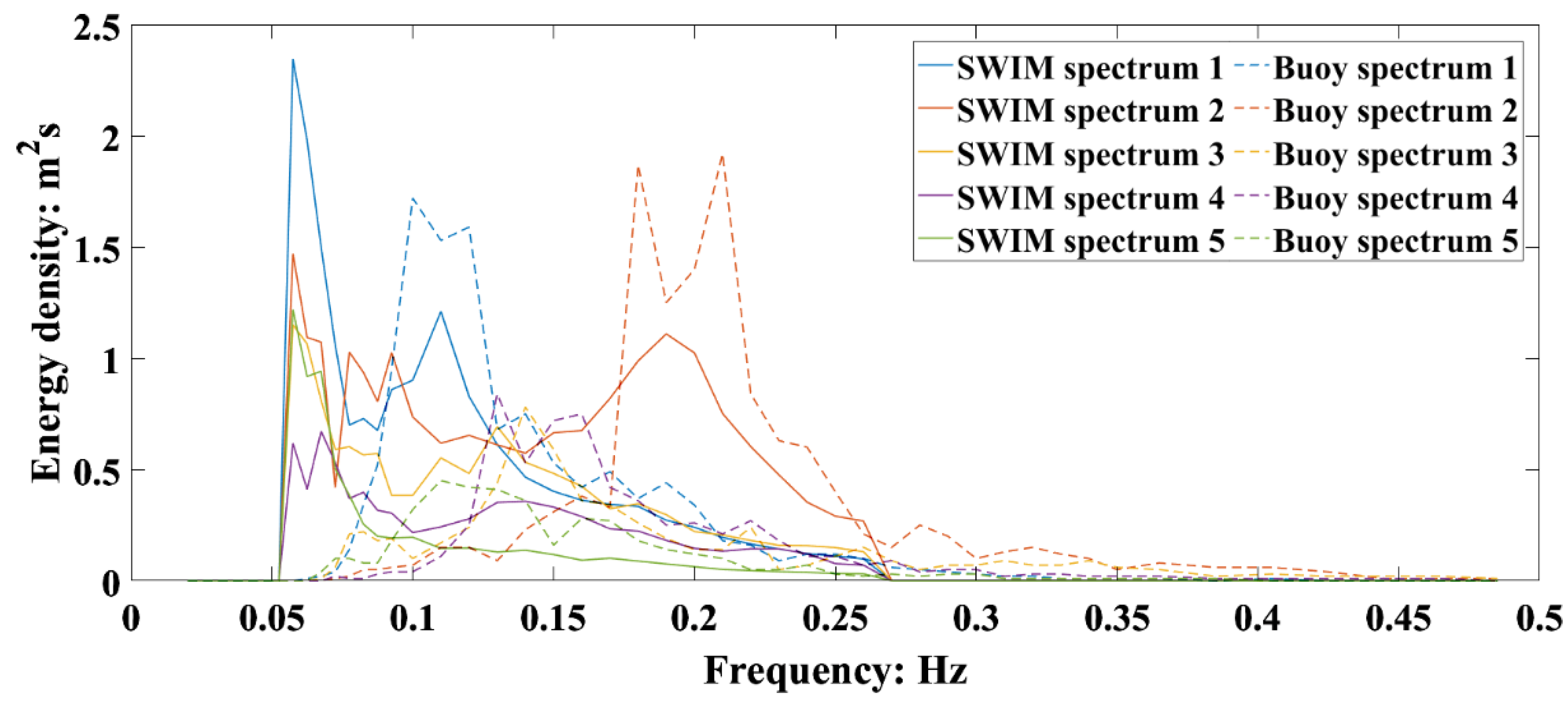
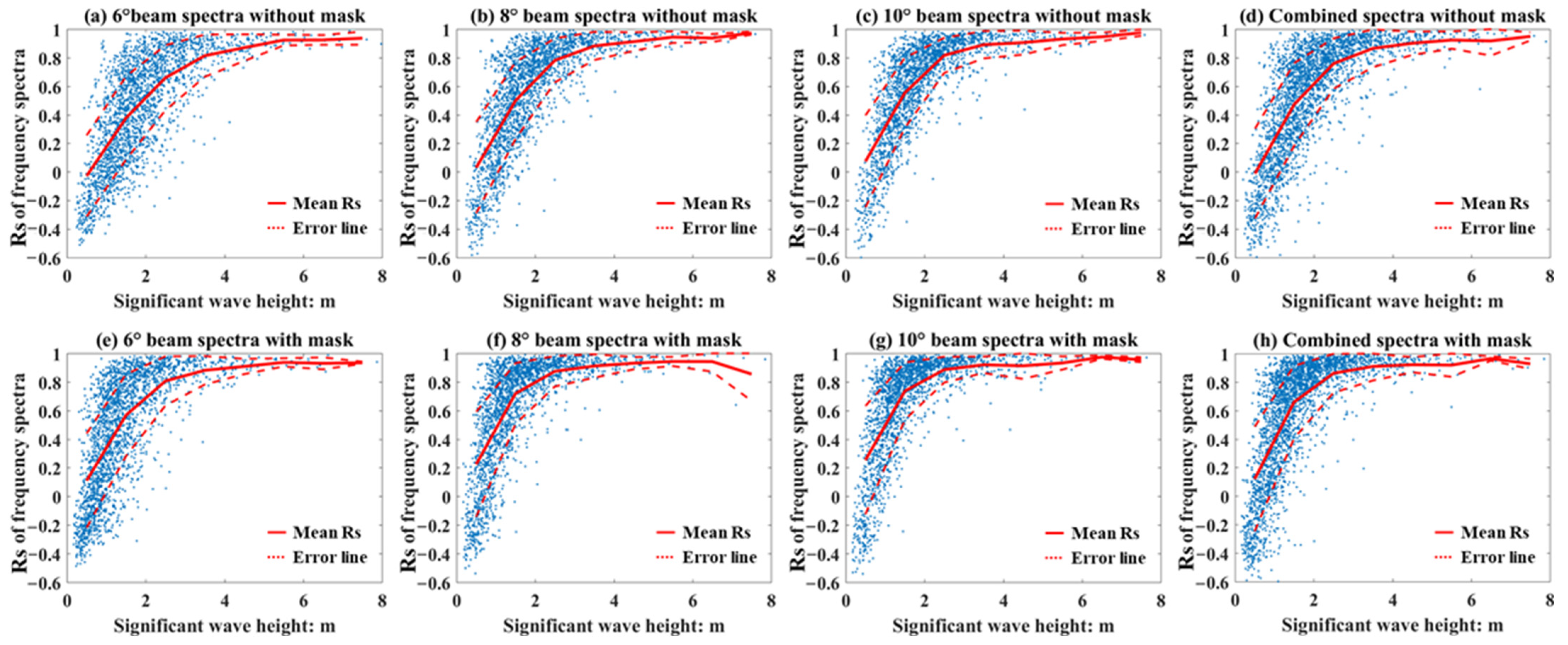
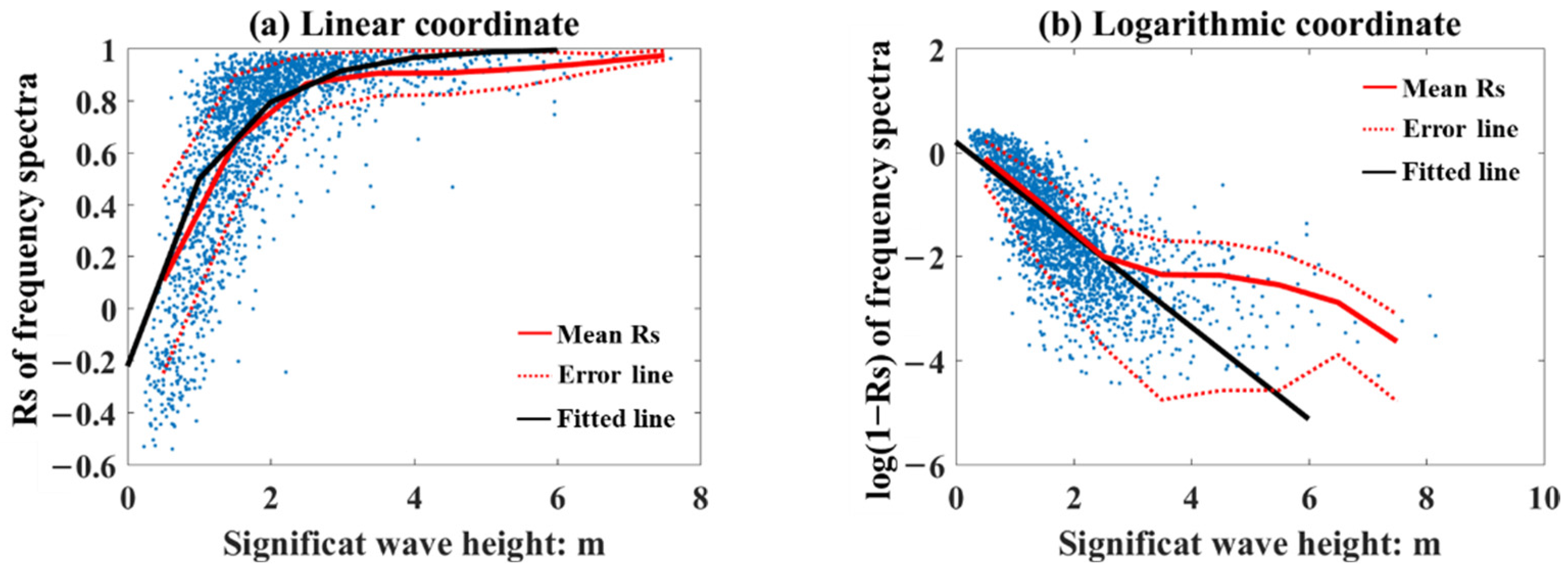
3.1. Error Analysis in Frequency Component
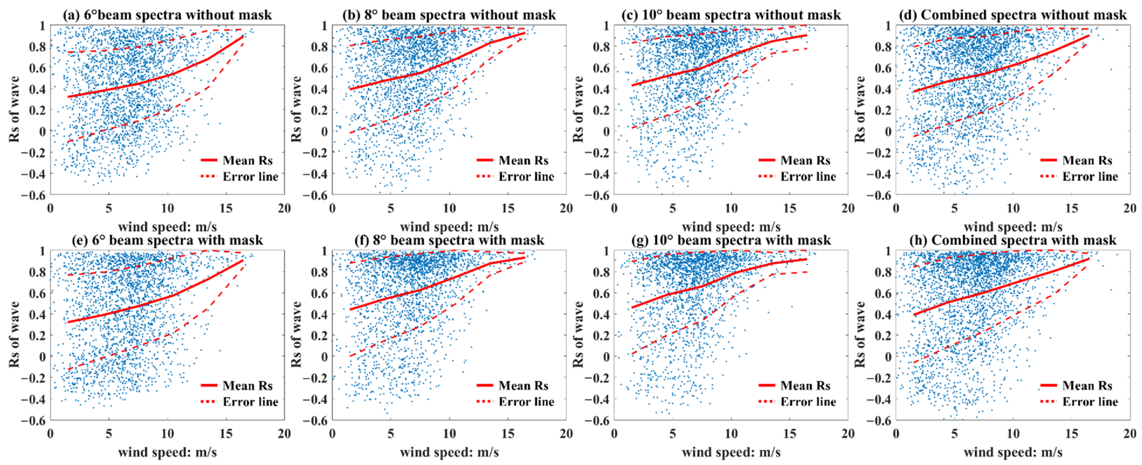
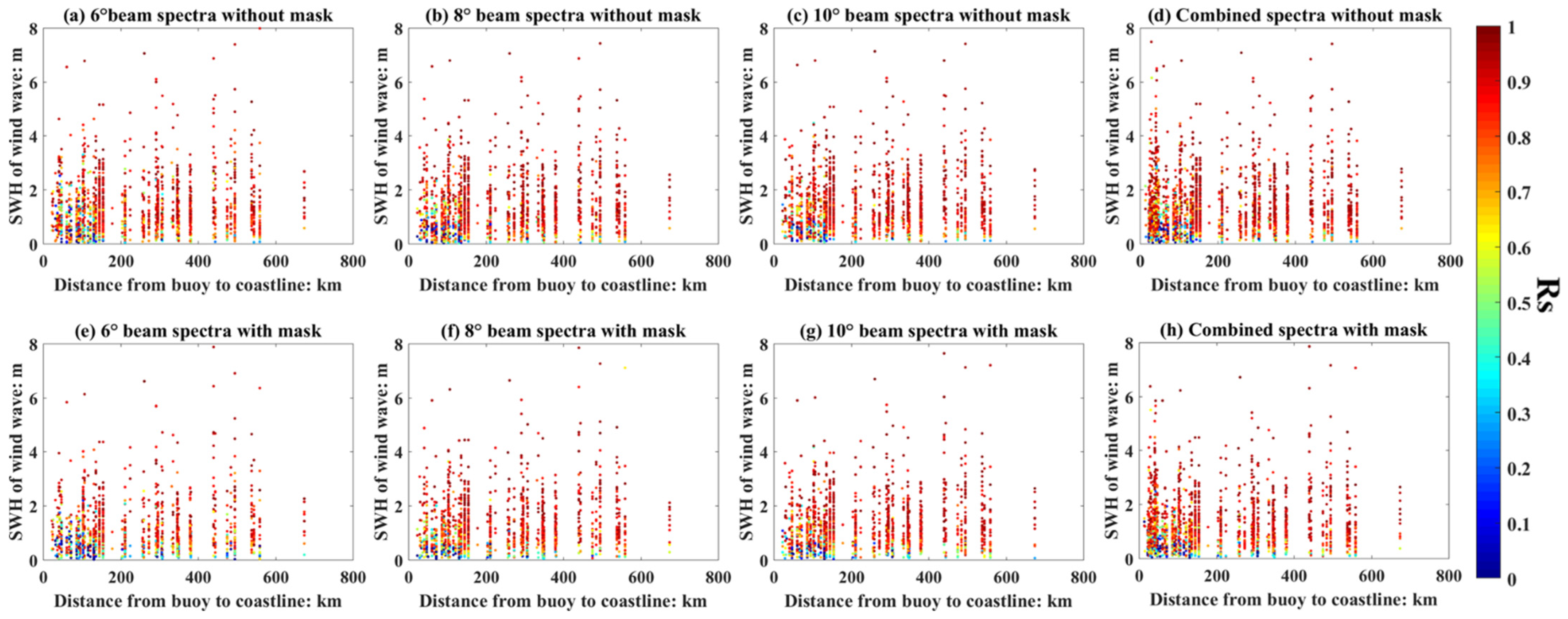
3.2. Factors That Impact the WS Accuracy
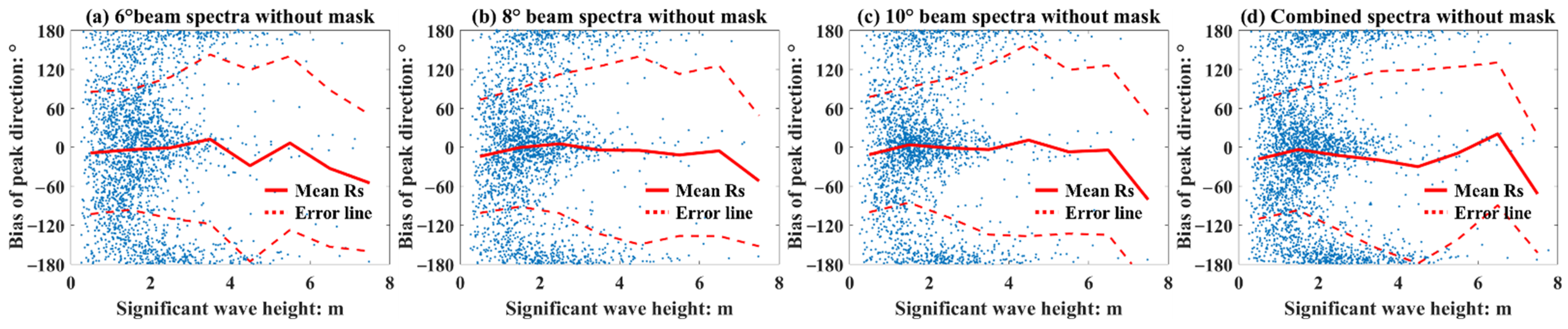
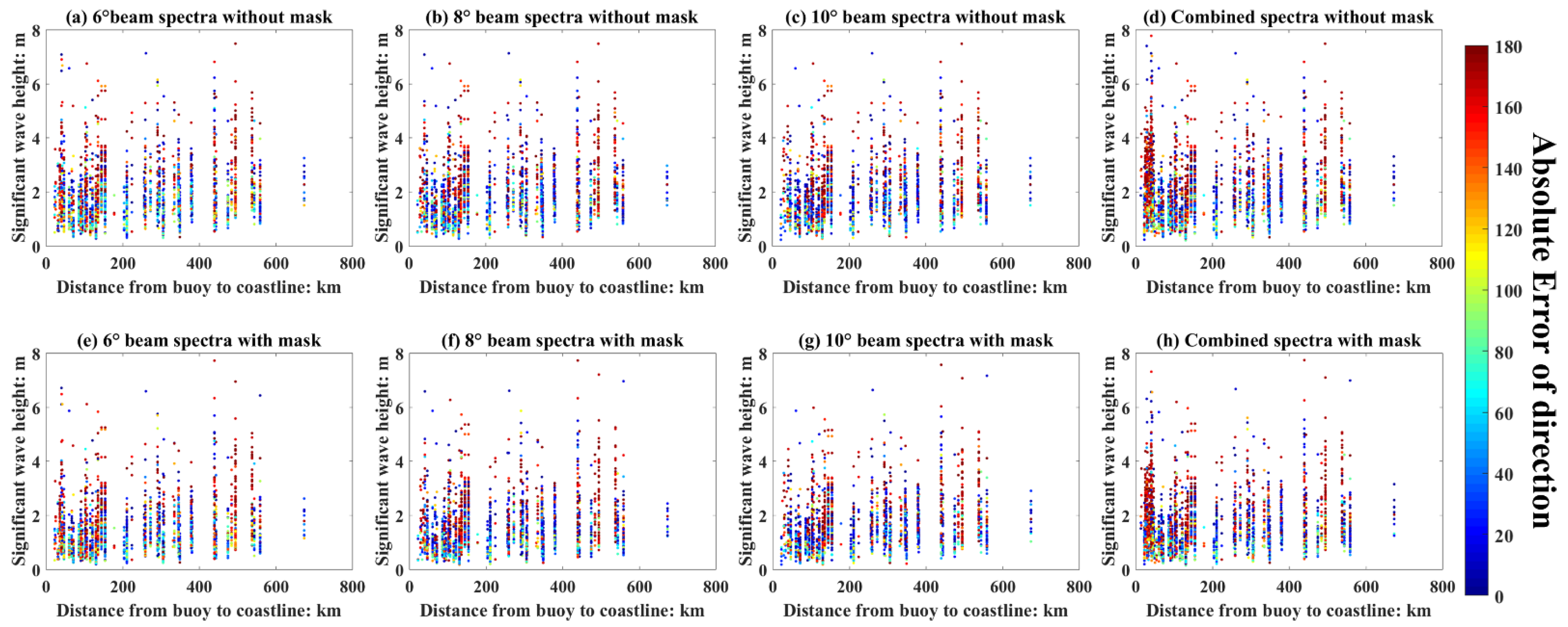
3.3. Error Analysis in Directional Component
4. Conclusions
Author Contributions
Funding
Data Availability Statement
Acknowledgments
Conflicts of Interest
References
- Ardhuin, F.; Marié, L.; Rascle, N.; Forget, P.; Roland, A. Observation and estimation of Lagrangian, Stokes, and Eulerian currents induced by wind and waves at the sea surface. J. Phys. Oceanogr. 2009, 39, 2820–2838. [Google Scholar] [CrossRef]
- Hsiao, S.C.; Chen, H.; Chen, W.B.; Chang, C.H.; Lin, L.Y. Quantifying the contribution of nonlinear interactions to storm tide simulations during a super typhoon event. Ocean Eng. 2019, 194, 10661. [Google Scholar] [CrossRef]
- Chang, T.Y.; Chen, H.; Hsiao, S.C.; Wu, H.L.; Chen, W.B. Numerical analysis of the effect of binary typhoons on ocean surface waves in waters surrounding Taiwan. Front. Mar. Sci. 2021, 8, 749185. [Google Scholar] [CrossRef]
- Barrick, D.E. Remote sensing of sea state by radar. In Remote Sensing of the Troposphere; Derr, V.E., Ed.; NOAA/Environmental Research Laboratories: Newport, RI, USA, 1972; pp. 186–192. [Google Scholar]
- Barrick, D.E. Extraction of wave parameters from measured HF radar sea-echo Doppler spectra. Radio Sci. 1977, 12, 415–424. [Google Scholar] [CrossRef]
- Lipa, B.J. Derivation of directional ocean-wave spectra by integral inversion of second-order radar echoes. Radio Sci. 1977, 12, 425–434. [Google Scholar] [CrossRef]
- Borge, J.C.N.; Reichert, K.; Dittmer, J. Use of nautical radar as a wave monitoring instrument. Coast. Eng. 1999, 37, 331–342. [Google Scholar] [CrossRef]
- Huang, W.M.; Wu, S.C.; Gill, E. HF radar wave and wind measurement over the Eastern China Sea. IEEE T. Geosci. Remote Sens. 2002, 40, 1950–1955. [Google Scholar] [CrossRef]
- Foreman, S.J.; Holt, M.W.; Kelsall, S. Preliminary Assessment and Use of ERS-1 Altimeter Wave Data. J. Atmos. Ocean. Tech. 1994, 11, 1370–1380. [Google Scholar] [CrossRef]
- Komen, G.J. Introduction to Wave Models and Assimilation of Satellite Data in Wave Models; European Space Agency Publications: Paris, France, 1985; Volume SP-244, pp. 21–26. [Google Scholar]
- Thomas, J.P. Retrieval of energy spectra from measured data for assimilation into a wave model. Q. J. R. Meteorol. Soc. 1988, 114, 781–800. [Google Scholar] [CrossRef]
- Esteva, D. Evaluation of preliminary experiments assimilating Seasat significant wave height into a spectral wave model. J. Geophys. Res. 1988, 93, 14099–14105. [Google Scholar] [CrossRef]
- Greenslade, D.J.M. The assimilation of ERS-2 significant wave height data in the Australian region. J. Marine. Syst. 2001, 28, 141–160. [Google Scholar] [CrossRef]
- Qi, P.; Fan, X.M. The impact of assimilation of altimeter wave data on wave forecast model in the north Indian Ocean. Marine Forecasts. 2013, 30, 70–78. [Google Scholar]
- Yu, H.M.; Li, J.Y.; Wu, K.J.; Wang, Z.F.; Yu, H.Q.; Zhang, S.Q.; Hou, Y.J.; Ryan, M.K. A global high-resolution ocean wave model improved by assimilating the satellite altimeter significant wave height. Int. J. Appl. Earth. Obs. 2018, 70, 43–50. [Google Scholar] [CrossRef]
- Hasselmann, S.; Lionello, P.; Hasselmann, K. An optimal interpolation scheme for the assimilation of spectral wave data. J. Geophys. Res. 1997, 102, 15823–15836. [Google Scholar] [CrossRef]
- Heimbach, P.; Hasselmann, S.; Hasselmann, K. Statistical analysis and intercomparison of WAM model data with global ERS-1 SAR wave mode spectral. J. Geophys. Res. 1998, 103, 7931–7977. [Google Scholar] [CrossRef]
- Sun, M.; Yang, Y.Z.; Yin, X.Q.; Du, J.T. Data assimilation of ocean surface waves using Sentinel-1 SAR during typhoon Malakas. Int. J. Appl. Earth. Obs. 2018, 70, 35–42. [Google Scholar] [CrossRef]
- Hasselmann, K.; Hasselmann, S. On the nonlinear mapping of an ocean wave spectrum into a synthetic aperture radar image spectrum and its inversion. J. Geophys. Res. 1991, 96, 10713–10729. [Google Scholar] [CrossRef]
- Yang, J.S.; Wang, H.; Huang, W.G.; Xiao, Q.M. Error analysis of Envisat ASAR level 2 algorithm based on simulation technique. In Proceedings of the 2007 IEEE International Geoscience and Remote Sensing Symposium, Barcelona, Spain, 23–28 July 2007. [Google Scholar] [CrossRef]
- Sun, J.; Kawamura, H. Retrieval of surface wave parameters from SAR images and their validation in the coastal seas around Japan. J. Oceanogr. 2009, 65, 567–577. [Google Scholar] [CrossRef]
- Mouche, A.; Chapron, B.; Johnsen, H.; Collard, F.; Wang, H.; Guitton, G.; Yang, J.; Husson, R. Perspectives for combining and exploiting ocean wave spectra measured from different space missions. In Proceedings of the 2016 IEEE International Geoscience and Remote Sensing Symposium (IGARSS), Beijing, China, 10–15 July 2016. [Google Scholar] [CrossRef]
- Aouf, L.; Hauser, D.; Tison, C.; Mouche, A. Perspectives for directional spectra assimilation: Results from a study based on joint assimilation of CFOSAT synthetic wave spectra and observed SAR spectra from Sentinel-1A. In Proceedings of the 2016 IEEE International Geoscience and Remote Sensing Symposium (IGARSS), Beijing, China, 10–15 July 2016. [Google Scholar] [CrossRef]
- Hauser, D.; Tison, C.; Amiot, T.; Delaye, L.; Corcoral, N.; Castillan, P. SWIM: The first spaceborne wave scatterometer. IEEE T. Geosci. Remote Sens. 2017, 55, 3000–3013. [Google Scholar] [CrossRef] [Green Version]
- Xiang, K.S.; Yin, X.B.; Xing, S.G.; Kong, F.P.; Li, Y.; Lang, S.Y.; Gao, Z.Y. Preliminary estimate of CFOSAT satellite products in tropical cyclones. IEEE Trans. Geosci. Remote Sens. 2021, 60, 1–16. [Google Scholar] [CrossRef]
- Li, X.Z.; Xu, Y.; Liu, B.C.; Lin, W.M.; He, Y.J.; Liu, J.Q. Validation and calibration of nadir SWH products from CFOSAT and HY-2B with satellites and in situ observations. J. Geophys. Res. 2021, 126, e2020JC01668. [Google Scholar] [CrossRef]
- Tang, S.L.; Chu, X.Q.; Jia, Y.J.; Li, J.M.; Liu, Y.T.; Chen, Q.; Li, B.; Liu, J.L.; Chen, W.Y. An appraisal of CFOSAT wave spectrometer products in the South China Sea. Earth. Space. Sci. 2022, 9, e2021EA002055. [Google Scholar] [CrossRef]
- Jiang, H.Y.; Mironov, A.; Ren, L.; Babanin, A.V.; Wang, J.K.; Mu, L. Validation of wave spectral partitions from SWIM instrument on-board CFOSAT against in situ data. IEEE Trans. Geosci. Remote Sens. 2021, 60, 1–13. [Google Scholar] [CrossRef]
- Grigorieva, V.G.; Badulin, S.I.; Gulev, S.K. Global validation of SWIM/CFOSAT wind waves against Voluntary Observing Ship data. Earth. Space. Sci. 2022, 9, e2021EA002008. [Google Scholar] [CrossRef]
- Hanson, J.L.; Phillips, O.M. Automated analysis of ocean surface directional wave spectra. J. Atmos. Ocean. Technol. 2001, 18, 277–293. [Google Scholar] [CrossRef]
- Mei, C.C. The Applied Dynamics of Ocean Surface Waves; Wiley: New York, NY, USA, 1983; p. 740. [Google Scholar]
- Jiang, H.Y.; Song, Y.H.; Mironov, A.; Yang, Z.; Xu, Y.; Liu, J.Q. Accurate mean wave period from SWIM instrument on-board CFOSAT. Remote Sens. Environ. 2022, 280, 113149. [Google Scholar] [CrossRef]
- Hauser, D.; Tourain, C.; Hermozo, L.; Alraddawi, D.; Aouf, L.; Chapron, B.; Dalphinet, A.; Delaye, L.; Dalila, M.; Dormy, E. New observations from the SWIM radar on-board CFOSAT: Instrument validation and ocean wave measurement assessment. IEEE Trans. Geosci. Remote Sens. 2021, 59, 5–26. [Google Scholar] [CrossRef]
- Earle, M.D. Development of algorithms for separation of sea and swell. Natl. Data Buoy Cent. Tech Rep MEC-87-1 Hancock County. 1984, 53, 1–53. [Google Scholar]
- Li, S.Q.; Zhao, D.L. Comparison of spectral partitioning techniques for wind wave and swell. Mar. Sci. Bull. 2012, 14, 24–36. [Google Scholar]
- Tourain, C.; Hauser, D.; Alraddawi, D.; Hermozo, L.; Suquet, R.R.; Schippers, P.; Aouf, L.; Dalphinet, A.; Dufour, C.; Lachiver, J.-M.; et al. Evolutions and Improvements in CFOSAT SWIM Products. In Proceedings of the 2021 IEEE International Geoscience and Remote Sensing Symposium IGARSS, Brussels, Belgium, 11–16 July 2021; pp. 7386–7389. [Google Scholar]


| Distance to Coastline: km | Number of Buoys | Percentage of Buoys | Number of Samples | Percentage of Samples |
|---|---|---|---|---|
| r < 50 | 44 | 44.9% | 598 | 20.5% |
| 50 ≤ r < 150 | 20 | 20.4% | 930 | 31.9% |
| 150 ≤ r < 300 | 13 | 13.3% | 554 | 19.0% |
| 300 ≤ r | 21 | 21.4% | 836 | 28.6% |
| Water Depth: m | Number of Buoys | Percentage of Buoys | Number of Samples | Percentage of Samples |
|---|---|---|---|---|
| d < 50 | 16 | 16.3% | 305 | 10.3% |
| 50 ≤ d < 500 | 38 | 38.8% | 807 | 27.4% |
| 500 ≤ d < 4000 | 24 | 24.5% | 837 | 28.4% |
| 4000 ≤ d | 20 | 20.4% | 999 | 33.9% |
| Spectra for Calculating the SWH | RMS of the SWH (m) | Bias of the SWH (m) | Std (m) | Mean Rs |
|---|---|---|---|---|
| 6° beam WFS (without mask) | 0.23 | 0.09 | 0.22 | 0.43 |
| 8° beam WFS (without mask) | 0.23 | 0.09 | 0.22 | 0.54 |
| 10° beam WFS (without mask) | 0.23 | 0.08 | 0.21 | 0.59 |
| Combined WFS (without mask) | 0.33 | 0.15 | 0.30 | 0.52 |
| 6° beam WFS (with mask) | 0.43 | −0.35 | 0.25 | 0.45 |
| 8° beam WFS (with mask) | 0.34 | −0.25 | 0.23 | 0.60 |
| 10° beam WFS (with mask) | 0.32 | −0.23 | 0.23 | 0.64 |
| Combined WFS (with mask) | 0.33 | −0.17 | 0.28 | 0.57 |
| Spectra for Calculating the SWH | RMS of the Wind Wave SWH (m) | Bias of the Wind Wave SWH (m) | Std of the Wind Wave SWH (m) | Mean Rs for Wind Wave |
|---|---|---|---|---|
| 6° beam WFS (without mask) | 0.31 | −0.21 | 0.23 | 0.77 |
| 8° beam WFS (without mask) | 0.27 | −0.16 | 0.22 | 0.80 |
| 10° beam WFS (without mask) | 0.24 | −0.10 | 0.21 | 0.82 |
| Combined WFS (without mask) | 0.29 | −0.12 | 0.27 | 0.79 |
| 6° beam WFS (with mask) | 0.66 | −0.59 | 0.29 | 0.71 |
| 8° beam WFS (with mask) | 0.47 | −0.41 | 0.23 | 0.76 |
| 10° beam WFS (with mask) | 0.40 | −0.34 | 0.21 | 0.78 |
| Combined WFS (with mask) | 0.44 | −0.36 | 0.25 | 0.75 |
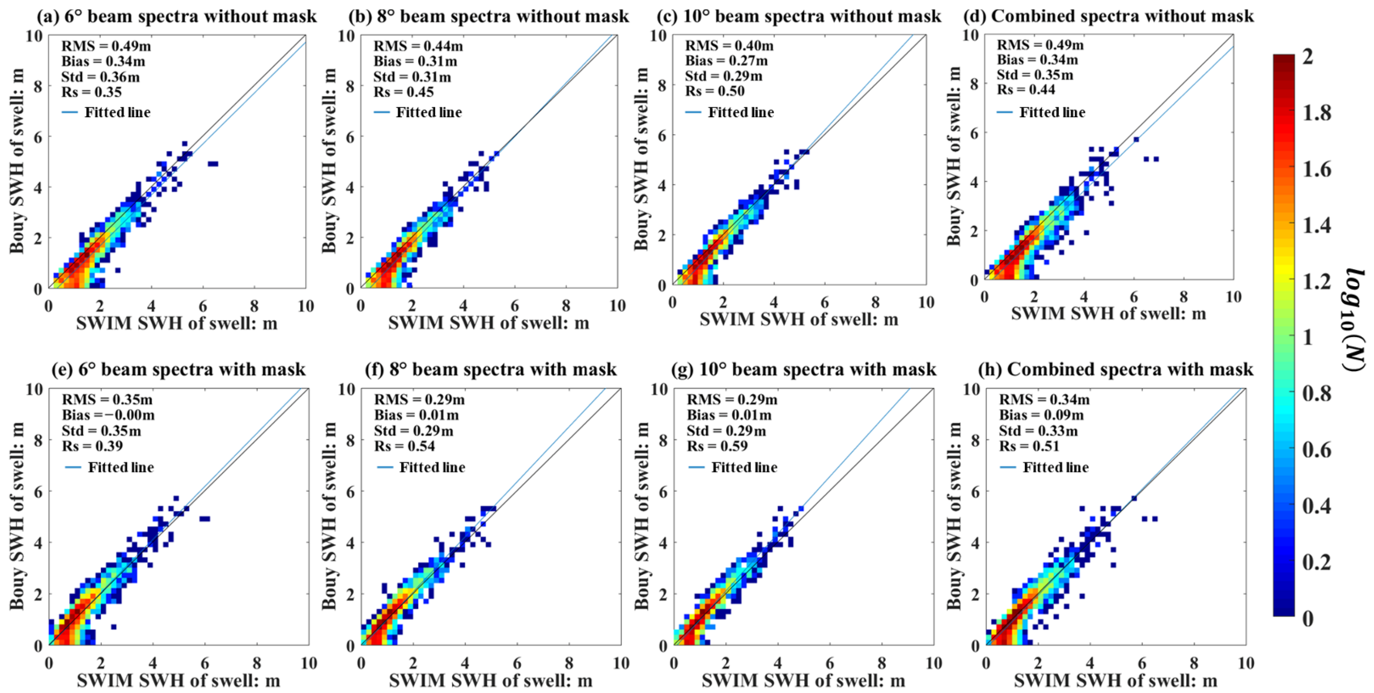
| Spectra for Calculating the SWH | RMS of the Swell SWH (m) | Bias of the Swell SWH (m) | Std of the Swell SWH (m) | Mean Rs for Swell |
|---|---|---|---|---|
| 6° beam WFS (without mask) | 0.49 | 0.34 | 0.36 | 0.35 |
| 8° beam WFS (without mask) | 0.44 | 0.31 | 0.31 | 0.45 |
| 10° beam WFS (without mask) | 0.40 | 0.27 | 0.29 | 0.50 |
| Combined WFS (without mask) | 0.49 | 0.34 | 0.35 | 0.44 |
| 6° beam WFS (with mask) | 0.35 | −0.00 | 0.35 | 0.39 |
| 8° beam WFS (with mask) | 0.29 | 0.01 | 0.29 | 0.54 |
| 10° beam WFS (with mask) | 0.29 | 0.01 | 0.29 | 0.59 |
| Combined WFS (with mask) | 0.34 | 0.09 | 0.33 | 0.51 |
Disclaimer/Publisher’s Note: The statements, opinions and data contained in all publications are solely those of the individual author(s) and contributor(s) and not of MDPI and/or the editor(s). MDPI and/or the editor(s) disclaim responsibility for any injury to people or property resulting from any ideas, methods, instructions or products referred to in the content. |
© 2023 by the authors. Licensee MDPI, Basel, Switzerland. This article is an open access article distributed under the terms and conditions of the Creative Commons Attribution (CC BY) license (https://creativecommons.org/licenses/by/4.0/).
Share and Cite
Li, S.; Yu, H.; Wu, K.; Yin, X.; Lang, S.; Ye, J. Validation of the Ocean Wave Spectrum from the Remote Sensing Data of the Chinese–French Oceanography Satellite. Remote Sens. 2023, 15, 3918. https://doi.org/10.3390/rs15163918
Li S, Yu H, Wu K, Yin X, Lang S, Ye J. Validation of the Ocean Wave Spectrum from the Remote Sensing Data of the Chinese–French Oceanography Satellite. Remote Sensing. 2023; 15(16):3918. https://doi.org/10.3390/rs15163918
Chicago/Turabian StyleLi, Songlin, Huaming Yu, Kejian Wu, Xunqiang Yin, Shuyan Lang, and Jiacheng Ye. 2023. "Validation of the Ocean Wave Spectrum from the Remote Sensing Data of the Chinese–French Oceanography Satellite" Remote Sensing 15, no. 16: 3918. https://doi.org/10.3390/rs15163918