Abstract
Feature extraction and recognition of underwater targets are important in military and civilian areas. This paper studied water surface acoustic wave (WSAW) detection by a millimeter wave (mmWave) radar. The mmWave-based endpoint detection method of the WSAW was introduced. Simulated results show that the continuous wavelet transform (CWT) method has a better detection performance. A 77 GHz large aperture antenna mmWave radar sensor and an underwater acoustic transmitter have been applied to conduct laboratory experiments. Still water surface experimental results verify that the CWT method has better detection capability, and the mmWave radar can accurately detect even 155 nm WSAW. Wavy water surface experimental results demonstrate the ability of the mmWave radar to analyze the time-frequency feature of the weak WSAW signal. These works indicate the potential of mmWave radar for the cross-medium detection and recognition of underwater targets.
1. Introduction
When sound waves are emitted toward the water surface, they will stimulate micro-vibrations on the water surface due to the mismatch between the specific acoustic impedances of the water–air interface. The sound-induced micro-vibration, whose particle vibration is between shear wave and longitudinal wave, propagates along the water surface and vibrates with the incident sound [1]. This micro-vibration is a kind of surface acoustic wave (SAW). The water surface acoustic wave (WSAW) contains acoustic transmission information of underwater targets and can play the role of a bridge that transmits underwater information to in-air equipment. Recently, human detection activities in the ocean have been increasing along with the continuous improvement of marine strategic status [2]. The detection of the WSAW can be used in searching and detecting noisy underwater equipment. Moreover, it also can be used in the active wireless cross-media information transmission of underwater equipment.
Because of its great significance, the related research of SAW detection has been underway for decades. The optic/laser technique was the first technique to be applied in SAW detection [3]. This technology is fully extended to the characteristics detection of the SWAW [4]. Acousto-optic technique-based WSAW detection has been studied via several techniques [5,6], including laser diffraction detection technology [7,8], laser slope scanning technology, laser interferometry technology, and laser phase scanning technology. In 1979, Weisbuch et al. [7] first proposed the realization of optical diffraction grating with a liquid surface wave and established the optical measurement method of surface tension. In 1988, Lee et al. [9] detected the sound-induced micro-vibrations with a laser. Interferometric techniques using coherent laser radiation to measure the acoustic signals on a vibrating surface have been successful [10]. An uplink underwater acoustic communication experiment was conducted in [11]. However, since the laser wavelength is very short, it is susceptible to water surface waves. Even when the water surface is calm, only a small amount of probe beam power will re-enter the interferometer [12]. In addition, the noise caused by a natural water surface seriously impairs the performance of the laser system. In the natural world, the water surface is full of waves. It is difficult to detect the WSAW using a laser outside the lab.
With the development of high-frequency radio wave radar, it has been found that millimeter wave (mmWave) radar can be used to detect the WSAW on fluctuating water surfaces. In 1972, Tremain and Angelakos detected underwater sound sources using 37 GHz microwave radiation reflected from the water surface. The experiment detected the 45 and 55 Hz WSAW with a maximum amplitude of either 0.16 cm or 0.08 cm [13]. In 2018, A 60 GHz mmWave radar was used to detect the WSAW and realize the cross-medium wireless communication [14]. Experimental results show that the mmWave radar-based technology can be applied to a few microns of a WSAW to communicate in the presence of surface waves with a max 16 cm peak-peak height, which is much higher than the wave heights allowed by a laser system.
The technology is verified again in [15]. Ref. [16] applied a 0.33 THz radar to detect 20 m WSAW. Ref. [17] used an improved Relax algorithm to detect the frequency of the WSAW. Compared with the acousto-optic technique, the mmWave-based WSAW detection technology has stronger robustness due to the longer wavelength of the mmWave. The amplitudes of waves on the natural wavy ocean surface are always 5–7 orders of magnitude larger than the sound-induced WSAW, which leads to unreliable unwrapping and echoes swaying. These significantly degrade the performance of WSAW detection through the natural water–air interface. The mmWave-based WSAW detection technology is expected to realize the WSAW-based underwater detection on the natural wavy water surface.
This paper focuses on endpoint detection of the WSAW. Endpoint detection of the WSAW is an important step in mmWave-based WSAW detection. The extremely weak WSAW signal is always submerged in huge water surface waves. In practical applications, it is usually required to judge whether there is a WSAW signal first, and accurately locate the starting point and ending point of the underwater sound signal. It helps to collect real underwater sound data, reduce the amount of data and computation, and reduce the processing time. Time–frequency analysis simultaneously studies a signal in both the time and frequency domains. In addition to facilitating endpoint detection, the time–frequency distribution can also be used for underwater sound signal feature extraction and recognition. Therefore, the research on the WSAW endpoint detection and time-frequency analysis algorithm is of great significance.
Here, the method for mmWave-based WSAW detection is analyzed. Simulation and experiment results are displayed to validate the potential of the technique. The rest of this paper is organized as follows. Section 2 describes the principle and system for the mmWave-based WSAW detection system. The algorithms for WSAW endpoint detection are introduced in Section 3. Section 4 gives the simulation methods and results. The experiments and discussions are described in Section 5. Section 6 concludes this paper.
2. Principle and System
2.1. WSAW Properties
The WSAW is a kind of micro-vibration of water particles. It occurs when underwater sound waves are incident on the water–air interface. The WSAW is between shear and longitudinal waves, propagating along the water surface. The displacement of the WSAW is small, and the effect of gravity can be ignored. Hence, the three-dimensional mathematical model of the WSAW with an ideal point sound wave at a horizontal plane XOZ can be written as [1]:
where z is the displacement, x and y represent horizontal coordinates, is the incident sound pressure at the water–air interface, is the density of water, is the sound frequency, and is the sound velocity in water. is an attenuation coefficient related to water viscosity, water surface tension coefficient, water density, and acoustic frequency. Figure 1 plots the three-dimensional WSAW excited by an ideal point sound wave.
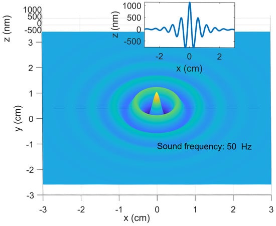
Figure 1.
Schematic diagram of ideal point source-induced WSAW.
Ignoring the horizontal attenuation, we can obtain the maximum vibration amplitude. The amplitude is linearly related to the incident sound pressure and can be calculated as:
The sound pressure level (SPL) range of marine sonar can be estimated by [18]:
where is the sound-radiated power, is the emission directivity coefficient. Generally, the radiated sound power of marine sonar is hundreds to thousands of watts, and the is 10 to 30 dB, so the SPL is approximately 210∼240 dB/. Considering a 500 m propagation attenuation as a spherical wave (propagation attenuation can be approximately estimated by , where d is the water depth in meters), the incident SPL at the water–air interface is approximately 120∼200 dB/. Figure 2 shows the amplitude of the sound-induced micro-vibrations with different incident SPLs and frequencies. It is shown that the amplitudes are very small (only a few hundred nanometers for 200 Hz sound with incident SPL 150 dB/).
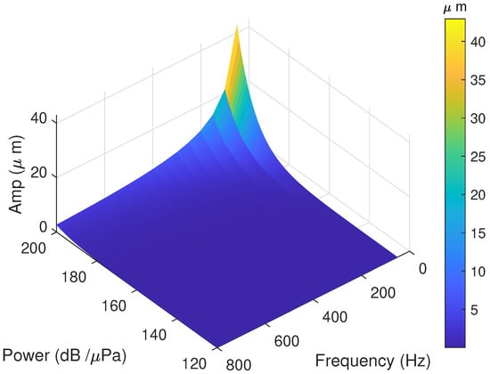
Figure 2.
Amplitude of the micro-vibrations with different incident SPLs and frequencies.
2.2. System
The WSAW detection system is composed of an underwater speaker as a transducer and a mmWave radar as a receiver. Figure 3 shows the configuration of the WSAW detection system by a mmWave radar. The underwater speaker can emit 80–8000 Hz sound, which is used to simulate the acoustic wave of underwater targets and stimulate the WSAW on the water–air interface. The mmWave frequency-modulated carrier wave (FMCW) radar transmits a wideband mmWave signal. It measures its reflection on the water surface, where the water surface has the WSAW, as Figure 3 shows.
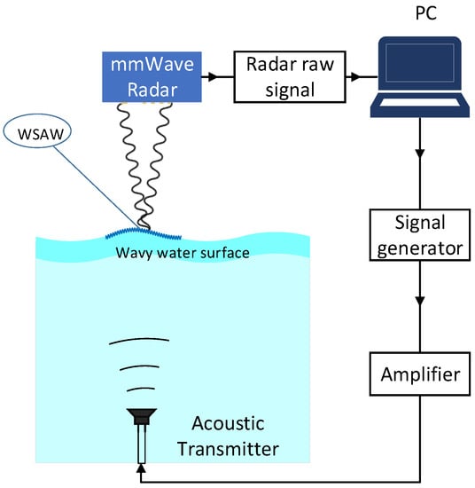
Figure 3.
Configuration of the mmWave based on the WSAW detection system.
2.3. mmWave Radar Detection Principle
The radar sensor is based on a linear FMCW architecture. It transmits a series of linear frequency-modulated waveforms, called chirps, with a period of T. In a sweep period T, the expression of the FMCW signal transmitted by mmWave radar can be expressed as:
where , represent the amplitude and random initial phase of the transmitted signal, respectively. is the carrier frequency, is the slope of frequency computed from the sweep bandwidth of B and the signal duration of T. At time t, a stationary target is at a distance r in front of the radar. The signal is reflected back from the target and returns back to the antenna in the form of , where is the round-trip delay of the echo calculated by: . The expression of the received target echo signal is:
where is the received target echo amplitude after propagation attenuation, c is the light speed, and is the initial phase of the received echo. Both the transmitted and received signals are mixed and low-pass filtered to produce an intermediate frequency (IF) signal that can be written as:
The last term of Equation (6) is known as the residual video phase and can be removed for the very small . Substitute into (6), the IF signal is obtained as:
The phase of the IF signal is . The phase changes can be used to detect the weak displacement of the target [19]. Here, our target is the WSAW. The signal phase from the water surface is:
where is the distance between the radar and the water surface, is the amplitude of the WSAW, and is the wavelength of the radar transmitted signal. Ignoring the influence of low-frequency water surface gravity waves, one can extract the high-frequency micro-vibrations (the WSAW signal) from the phase changes of . Figure 4 gives the phase changes for a 77 GHz mmWave radar with different sound frequencies and incident powers.
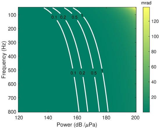
Figure 4.
Phase changes with different SPLs and frequencies for a 77 GHz mmWave radar. The white curve is the contour that has a constant phase change. For example, the curve labeled 1 represents a phase change of 1 mrad.
2.4. Radar Signal Preprocessing
The FMCW radar measures the reflection after a fast Fourier transform (FFT)-based range compression. Generally, the highest reflection power range bin is chosen to extract the phase of each chirp. The extracted phase is wrapped due to the surface waves. The wrapped phase needs an unwrapping process before the next process. Spline interpolation is used to fill the missing data, if necessary. Then, a high-pass filter is applied to eliminate the low-frequency modulation of water surface waves. The surface waves always induce spikes which degrade communication performance significantly and are difficult to filter out. After this processing, the signal feature can be extracted from the filtered phase signal. Finally, the WSAW endpoint can be obtained by a decision method. Signal processing steps are presented in Figure 5.
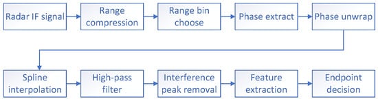
Figure 5.
Signal processing flow diagrams.
3. Algorithms for WSAW Endpoint Detection
The WSAW signal is weak, while the natural waves are huge. The WSAW signals are always submerged in water surface fluctuation or even in the phase noise of a radar system. Hence, it is difficult to judge its existence and endpoint position directly. The accuracy detection of the WSAW endpoint in various noise environments is particularly important for practical applications. Here, we refer to the general sequential signal processing method and show the feature extraction method and endpoint decision strategy of the WSAW signal.
3.1. Feature Extraction
The general time series endpoint detection is based on the feature extraction in time domain, frequency domain, time-frequency domain, and cepstrum domain [20]. The traditional short-time energy (STE) algorithm, Hilbert Huang transform (HHT) algorithm, and continuous wavelet transform (CWT) algorithm are tested in this paper. Next, we will give a brief introduction to these algorithms.
3.1.1. Short-Time Energy Algorithm
The STE algorithm is a simple and widely applied algorithm based on the average energy over a sliding window of length L across neighboring elements of a signal [21]. The STE can be calculated as:
The algorithm can effectively reduce noise energy and amplify signal energy. Due to the weak WSAW signal, the higher-order short-time energy algorithm is applied here to achieve a better detection result, as:
Short-time Fourier transform (STFT) is a basic time-frequency analysis method that can be used to analyze how the frequency content of a nonstationary signal changes over time. It produces a time-frequency spectrum by taking the Fourier transform over a chosen time window. In STFT, the time-frequency resolution is fixed over the entire time-frequency space by preselecting a window length. Therefore, resolution in data analysis becomes dependent on window length.
3.1.2. Hilbert Huang Transform (HHT) Algorithm
HHT was applied in accurate underwater acoustic signal frequency estimation using an acousto-optic technique [22]. As a novel and effective method for processing nonlinear and nonstationary signals, the HHT method has been gradually applied in various fields, such as seismic signal analysis, ocean signal analysis, wind speed analysis, bridge health monitoring, voice signal processing, graphic image processing and analysis, and in biomedicine and so on [23,24,25]. HHT is an adaptive time-frequency analysis method of non-stationary signals based on data. This method is based on the Hilbert transform (HT) [26]. The basic idea of HHT is to use empirical mode decomposition (EMD) to decompose the signal into a limited number of intrinsic mode functions according to certain screening criteria [27]. Here, the HHT method decomposes the unwrap phase signal by the EMD, obtains the Hilbert energy spectrum of the signal through adaptive weight selection of the inherent mode function [28,29], and uses the sequential statistical filter to smooth the energy spectrum as the distinguishing feature of the WSAW signal.
3.1.3. Continuous Wavelet Transform (CWT) Algorithm
CWT uses inner products to measure the similarity between a signal and an analyzing function [30]. The CWT compares the signal to shifted and compressed or stretched versions of a wavelet. Stretching or compressing a function is collectively referred to as dilation or scaling and corresponds to the physical notion of scale. By comparing the signal to the wavelet at various scales and positions, a function of two variables is obtained. There are many different admissible wavelets that can be used in the CWT. Generalized Morse wavelet is a two-parameter family of functions, and it can be used to build up a time series [31]. Generalized Morse wavelets are a family of exact analytic wavelets. They are useful for analyzing modulated signals, which are signals with time-varying amplitude and frequency. They are also useful for analyzing localized discontinuities [32]. The Morse wavelets, represented as , are defined in the frequency domain for and as:
where is angular or radian frequency, is the unit step, and is a real-valued normalized constant chosen as
The parameter , called the order, controls the low-frequency behavior, which can be viewed as a decay or compactness parameter. While , called the family, controls the high-frequency decay and characterizes the symmetry of the Morse wavelet. is the time-bandwidth product. By adjusting the time-bandwidth product and symmetry parameters of a Morse wavelet, one can obtain analytic wavelets with different properties and behavior. A strength of Morse wavelets is that many commonly used analytic wavelets are special cases of a generalized Morse wavelet. The (demodulate) skewness of the Morse wavelet equals 0 when . The wavelet transform of a square-integrable signal with respect to the wavelet is defined in the frequency domain as:
where is the Fourier transform of , is the scale factors, s is the position factors, and the asterisk denotes the complex conjugate. Here, we use the parameters as . To further improve algorithm performance, the high-order energy of the CWT decomposed parameters is extracted as a feature by:
3.2. Decision Method
An adaptive endpoint detection method is proposed to determine the final endpoint position. The decision method is as follows:
- (1)
- Setting the lengths of reference and protection units.The length is set according to the length of the WSAW and the power ratio of WSAW phase signal to the noise phase signal (SNR). Without losing generality, we set the length of reference units as 40, and the length of the protection unit is 4.
- (2)
- For the edge value (the first and last 40 points), the lengths of the reference unit are less than the setting value.
- (3)
- Calculating the left and right median values within the reference units.
- (4)
- Calculating the difference between the left and right median values.
- (5)
- Setting edge protection by setting the first and last 50 difference points values as 0.
- (6)
- Finding the maximum and minimum values of the median difference between the two sides.
- (7)
- Making the maximum and minimum difference as the endpoint.
Figure 6 shows the decision method architecture with the length of reference unit of 40 and the length of protection unit of 4. Figure 7 gives the detailed signal processing flow diagrams of the decision method based on the extracted feature signal. The two-parameters method can adaptively identify the step change of the extracted feature signal.
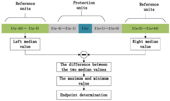
Figure 6.
The decision method architecture with the length of reference units of 40 and the length of protection unit of 4.
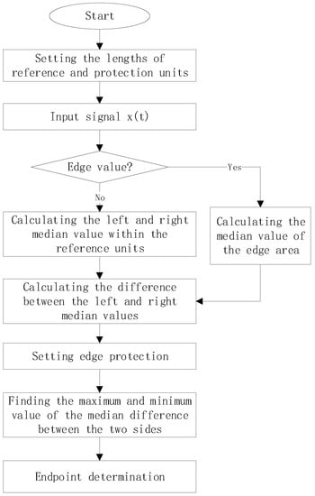
Figure 7.
Signal processing flow diagrams of decision method.
4. Simulation Test
To evaluate the performance of the algorithm in different scenarios, we simulate the radar-received echo data based on different wavy ocean surfaces. In the simulation process, we assume that the water surface waves are wind-induced and the unwrapping phases of the radar echo correspond to the single point fluctuation of the water surface.
4.1. Wavy Ocean Surface Simulation
According to the linear wave theory, the randomly varying ocean surface can be treated as the superposition of a series of single waves with different amplitudes, frequencies, and propagation directions. Hence, the instantaneous water surface elevation corresponding to a point can be calculated by:
where n is the number of unit waves, is the amplitude, is the angular frequency, is the wavenumber of spatial frequency, and is the initial wave phase angle, which is generally generated randomly. In a stationary random process, their spectral density function or wave spectrum is defined as the Fourier transform of the correlation function of rough surface waves. The wave spectrum can be used to estimate the value of and to simulate the instantaneous water surface elevation. Here, the classical PM spectrum wave spectrum is used to simulate the random wave surface [33] as
where k is the wave number, g is the acceleration of gravity, and is the wind speed of 19.5 m high on the surface. Since the phase velocity of the capillary wave is small, the capillary wave-induced phase change in radar echoes has a lower frequency than that of the WSAW. Furthermore, capillary wave-induced phase change can be filtered out by the high-pass filtering process. Consequently, the influence of capillary waves is ignored here. After the wave spectrum is discretized, the parameters of each unit wave can be obtained. The classical fast Fourier transform (FFT) can be used to generate random rough surface samples faster. The elevation of the rough surface at any position can be expressed as:
where is the root square amplitude of the wavenumber spectrum, L is the length of the simulated ocean surface size , and M is the number of eigenvalues. The specific conversion process is described in [34].
Figure 8 shows the 1D ocean surface retrieved under different wind speeds with 4,194,304 points. The simulation has a 50 m patch size and a spatial wavenumber resolution of 0.1257 rad/m. The sample frequency is 10 kHz, and there are 60,000 samples in total. The wind speeds of the three diagrams are 2 m/s, 4 m/s, and 6 m/s, respectively. The simulated water surface fluctuation is consistent with the actual water surface fluctuation characteristics.
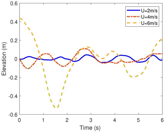
Figure 8.
One-dimensional (1D) ocean elevation time series at a position retrieved under different wind speeds.
4.2. Algorithms Simulation
The 77 GHz mmWave is applied in the simulation with the phase sensitivity of 1.61 rad/mm. At the same time, there are 2 s WSAW signals with different intensities, and −73 dBW ADC quantization caused Gaussian noise in the radar phase data. Figure 9 shows the simulated phase data. Figure 9a presents the unwrapping phase of the radar echo, which corresponds to the single point fluctuation of the water surface at 2 m/s wind speed. The middle red line area represents that the phase contains weak 2 s 200 Hz sinusoidal WSAW signal. Figure 9b presents the high-pass filtered and interference peak removed unwrapping phase of the radar echo. The SNR, the power ratio of the WSAW phase signal to the noise phase signal, is about 7.93 dB.
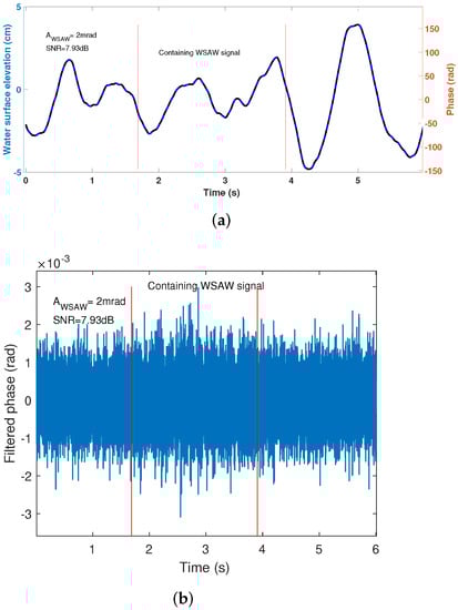
Figure 9.
Simulation radar phases; (a) Surface elevation; (b) Filtered phase.
Figure 10 shows the extracted features and endpoint decision results obtained by the STE, HHT, and CWT methods. The red lines show the actual endpoint location, and the green star lines show the determined endpoint location. For the same phase data shown in Figure 9b, the CWT method can get the best endpoint decision result, while the short-time energy method cannot give the right endpoint location. It is worth noting that both HHT and CWT methods have applied the frequency-domain energy distribution, which effectively improves the detection accuracy.
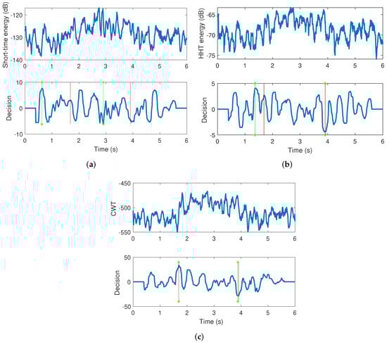
Figure 10.
Feature extraction and decision result of the simulated data, the red lines show the actual endpoint location and the green star lines show the determined endpoint location; (a) STE; (b) HHT; (c) CWT.
In order to verify and compare the detection performance with different WSAW phases (the amplitudes of the WSAW), we simulated the endpoint detection probabilities of the three methods. Table 1 gives the simulation detection rates for three methods under 2 m/s wind speed with 1000 randomly fluctuating water surfaces. When the difference between the estimated and the actual endpoints is fewer than 0.1 s (1000 points for 10 KHz time sampling frequency), we considered that the endpoint has been successfully detected. It can be seen that, with the increase of the WSAW phase, the detection probability increases. As in the previous analysis, the detection performance of the CWT method is the best, followed by that of the HHT and STE methods. Table 2 presents the WSAW phase and the corresponding amplitude of the WSAW. When the WSAW phase is 0.5 mrad, the amplitude of the WSAW is only 155 nm. It is challenging to detect such weak vibration on the water surface at a wind speed of 2 m/s, as Table 1 shows. For a 775 nm WSAW, the endpoints can be detected on a wavy surface.

Table 1.
Simulation detection rates with 2 m/s wind speed.
Table 2.
The WSAW phase vs. amplitude.
The detection performances are also verified and compared under different wind speeds. Due to the complexity and rapid changes of waves on the water surface, the impact of water surface waves is significant and complex. The deviation of the echo caused by water surface waves may result in the failure of receiving the echo or the absence of the WSAW signal in the radar echo. In these cases, none of the three algorithms can detect the endpoint of the WSAW signal. The impact of multipath interference on the received radar echo is more complex, which is related to the fluctuation state of the water surface and the design of the radar system. Generally, the greater the waves of the water surface, the more significant and frequent the occurrence of non-Gaussian impulsive noise in the radar echo. Accurate analysis and simulation of their impact are difficult and challenging. Hence, we simplify the impact of waves uisng an -stable process [35,36,37], as shown in Figure 11. Here, the -stable processes with = 0.5, 1.2, and 1.7 correspond to the wave-induced impulsive noise at 2 m/s, 4 m/s, and 6 m/s wind speeds, respectively. The simulated impulsive noise is normalized by and added in the simulated radar unwrapping phase as shown in Figure 9b. It can be seen that, as the wind speed increases, the frequency and intensity of the impulsive noise show a significant increase. Table 3 gives the simulated detection rates at different wind speeds. The performance of all three methods decreases with increasing wind speed, especially when the wind speed is 6 m/s. Overall, the CWT method has a better detection performance.
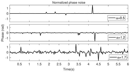
Figure 11.
Simulating phase impulsive noise modeled as an -stable process. Different indicates different wind speeds. , , and corresponds to 2 m/s, 4 m/s, and 6 m/s wind speeds, respectively.
Table 3.
Simulation detection rates at different wind speeds (different ) with 2.5 mrad WSAW phase.
5. Experiment and Discussion
5.1. Experiment Describtion
A laboratory experiment is conducted to verify the above analysis. A general Texas Instrument on-chip mmWave FMCW radar AWR1243 and an underwater acoustic transmitter are implemented in our experiment, as shown in Figure 12a. The AWR1243 device is an integrated single-chip FMCW transceiver capable of operating in the band of 76 to 81 GHz. It enables a monolithic implementation of a three transmitter and four receiver channels radar system [38]. To increase the antenna aperture and antenna beam gain, the two channels of the transceiver are designed as 16 × 16 and 32 × 32 microstrip patch array antennas, with beam widths of × and , respectively. Figure 12b shows the mmWave FMCW radar system. During this experiment, we used the parameter settings of radar shown in Table 4. The mmWave radar is mounted above a 128 cm × 55 cm × 65 cm water tank. It is about 80 cm above the water surface, and the acoustic transmitter is 13 cm below it. The underwater transmitter has a conversion efficiency of 105 dB/w/m and is excited by a 120 W power amplifier. A 200 Hz sinusoidal tone is transmitted by the underwater acoustic transmitter. Figure 12a shows the experimental scene.
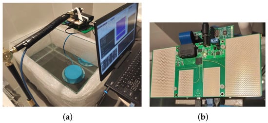
Figure 12.
(a) Experimental scene diagram; (b) Millimeter-wave radar with microstrip patch antenna array.
Table 4.
Radar parameters.
5.2. Experiment Results on Still Water Surface
Typical experimental results on the still water surface are presented in Figure 13. Figure 13a shows the results of range compression (FFT) by the data of the microstrip patch array antenna channel. Here, the 8th range bin indicates the reflection from the nearest water surface with the max reflection power. Note that the light points indicate relatively strong echoes. Figure 13b gives the unwrapped phase series of the 8th range bin, and Figure 13c is the high-pass filtered phase of the unwrapped results in Figure 13b. The phase series in Figure 13b,c contains the WSAW signal; however, it is too small to be seen. After high-pass filtering, the high-frequency WSAW signal is submerged in high-frequency noise, as shown in Figure 13c.
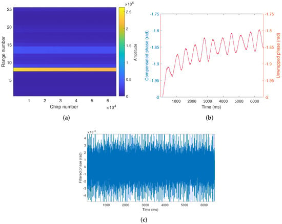
Figure 13.
Signal process results; (a) Range vs. Chirp number matrix; (b) Unwrapped and compensated phase; (c) Filtered phase.
In the experiment, the duration (6.5 s) of radar transmission is longer than that (2.1 s) of the sound wave. The mmWave is transmitted first and then the sound wave, which ensures that the radar echo can perceive the WSAW signal. However, when the WSAW signal is small, it is difficult to directly judge whether the WSAW exists and the occurrence time points by the unwrapped and filtered phases. Figure 13c shows that the WSAW-caused phase change is below 0.5 mrad, which means that the amplitude of the WSAW is below 155 nm as shown in Table 2. The estimated SNR of the filtered phase is about −10 dB.
Figure 14 shows the endpoint detection results from the STE algorithm of the filtered phase signals at the 8th range cells. The results show that the WSAW signal is difficult to extract directly from the time-series data. Frequency domain information can greatly improve the performance of endpoint detection. Figure 15, Figure 16 and Figure 17 present the three kinds of time-frequency mappings and their endpoint detection results. STFT and CWT can achieve the right endpoint detection results among the three kinds of time-frequency analysis. Compared with STFT, CWT can achieve more precise time-frequency analysis results. In Figure 17a, a highlighted spectral line can be seen at 200 Hz. The highlighted spectral line lasts about 2 s, corresponding to the continuous 2.1 s 200 Hz WSAW signal. The STFT and CWT time-frequency mappings show that the high-frequency noise mainly ranges from 300 Hz to 1000 Hz.
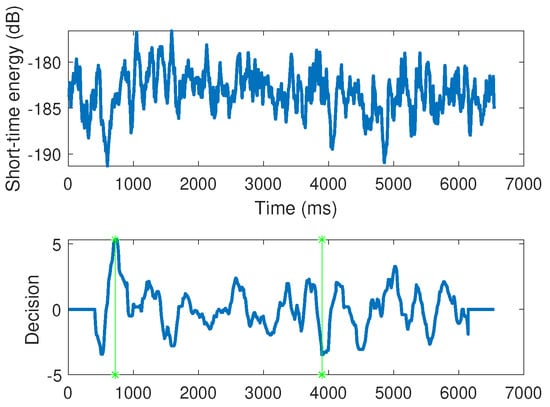
Figure 14.
Endpoint detection results by short-time energy algorithm, the green star lines show the determined endpoint location.
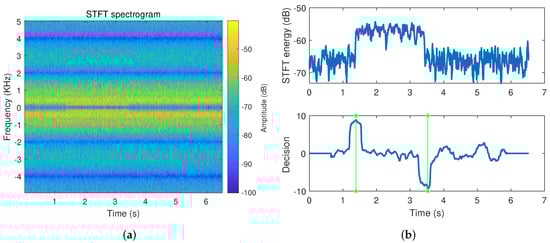
Figure 15.
(a) STFT spectrogram; (b) Endpoint detection results by the STFT spectrogram.
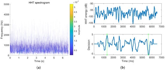
Figure 16.
(a) HHT spectrogram; (b) Endpoint detection results from the HHT spectrogram.
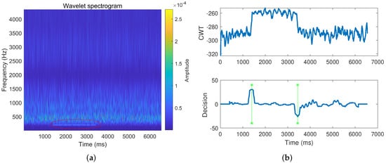
Figure 17.
(a) CWT spectrogram; (b) Endpoint detection results from the CWT spectrogram.
5.3. Experiment Results on Wavy Water Surface
Experimental results on a wavy water surface are presented in Figure 18. Figure 18a shows the results of range compression (FFT) from the data of the microstrip patch array antenna. Here, the 8th range bin also indicates the reflection from the nearest water surface with the max reflection power because the wave peak–peak amplitude is below the range resolution. Figure 18b shows the unwrapped phase series of the 8th range bin and the high-pass filtered phase of the unwrapped results. The unwrapped phase series indicates that the wave peak-to-peak amplitude is about 0.5 cm on the water surface. Here, the underwater speaker transmits a linear frequency modulation (LFM) signal from 100 Hz to 1000 Hz during 2.1 s. The phase series in Figure 18b contains the LFM WSAW signal, although the LFM WSAW signal is submerged in high-frequency noise and is hardly seen.
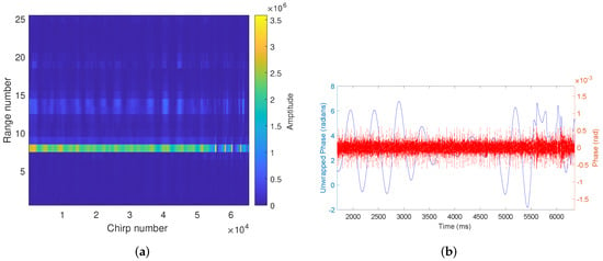
Figure 18.
Signal process results; (a) Range vs Chirp number matrix; (b) Unwrapped phase and high-pass filtered phase.
Due to strong noise and signal expansion in the frequency domain, the endpoints are difficult to detect directly. Figure 19 shows the time-frequency distribution of the filtered phase signal. Figure 19a gives the STFT spectrogram. The spectrogram uses a Hann window of length 128 and 96 overlapped samples for each window. The 128 points DFT was calculated with a fixed frequency resolution of 78 Hz. In the spectrogram, a weak short oblique line can be seen at the time of 2 s; this is the time-frequency distribution of the LFM signal. Because the LFM signal is weak and the noise is too strong, most LFM spectrum distribution is submerged in the noise.
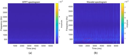
Figure 19.
LFM signal in time-frequency spectrum; (a) STFT spectrogram; (b) CWT spectrogram, the red circle indicates the spectrogram of the WSAW signal.
Figure 19b presents the CWT spectrogram. The spectrogram is also obtained using the analytic Morse wavelet with a symmetry parameter (gamma) equal to 3 and the time-bandwidth product equal to 60. The minimum and maximum scales are determined automatically based on the energy spread of the wavelet in frequency and time. In the spectrogram, the oblique line at the time around 2 s represents the time-frequency distribution of the LFM signal. This oblique line is relatively clear and longer than that in the STFT spectrogram. The STFT technique suffers from the fixed time and frequency resolution due to the fixed window length used in the analysis, limiting its applications in practice. The frequency resolutions of the CWT spectrogram are variable, and about 8 Hz around 100 Hz, and 50 Hz around 1000 Hz. When the signal is less than 1 kHz, CWT has a finer frequency resolution than the STFT. Therefore, CWT has a stronger time-frequency analysis ability of the WSAW signal than the STFT.
In the two spectrograms, the visible duration of the LFM signal is only about 1 s, while the total duration of the transmitting sound wave lasts 2.1 s. This phenomenon is mainly because the WSAW amplitude is inversely proportional to the frequency, as Equation (2) shows. The high-frequency WSAW corresponds to a smaller amplitude, that is, a weaker signal. Hence, high-frequency (>500 Hz) signals are submerged in noise.
In this data set, the water surface waves are small and there is no waves-induced high-frequency interference signal. This means that the mmWave radar can detect the below-155 nm WSAW signal. When the water surface fluctuation becomes large, mmWave radar cannot detect such a weak WSAW signal and the strength of the WSAW needs to be increased, as Table 1 shows.
5.4. Discussions
The optic technologies are not only sensitive to ambient light but are also more susceptible to water surface interference than radar technology for its short wavelength. Due to these limitations, the current optic technologies mainly conduct researches and experiments on single-frequency or multi-frequency signal cross-medium detection in the laboratory environment [1,39]. Laser interferometry technology has the advantages of high sensitivity and bandwidth. However, it still has problems with detecting low-frequency underwater sound in real-time on natural water surfaces. In 2017, this technology achieved the real-time detection of underwater targets with acoustic frequencies ranging from 300 Hz to 19 kHz in an optical darkroom [22]. The mmWave-based cross-medium detection technology can be used to detect low-frequency underwater sound sources (<200 Hz) undisturbed. It is more capable of detecting the WSAW on the actual sea surface.
These experiments realized the detection of the WSAW with a minimum amplitude below 155 nm. It infers the potential of detecting sound sources in deep water by mmWave radar. As shown in Figure 4 and Equation (3) above, the low-frequency underwater sound wave (below 200 Hz) at a depth of 100 m can be detected by this mmWave radar. The detection sensitivity is much better than the previous microwave detection results, and even closer to the laser detection sensitivity (about 60 nm [40]), as shown in Table 5. This work indicates the potential of mmWave radar for the cross-medium detection of underwater sounds in an actual ocean surface environment.
Table 5.
Comparison of main experiments of cross-medium detection/communication [13,14,15].
6. Conclusions
The feature extraction and recognition of underwater targets have a wide range of needs whether in military or civilian areas. This paper studied the WSAW endpoint detection using a mmWave radar. Three algorithms for the feature extraction were tested. A decision method for the WSAW endpoint was introduced. Simulation results under different wind speeds validate the decision method and indicate that the CWT algorithm has a better detection performance. A system that combines a 77 GHz large aperture antenna mmWave radar sensor and an underwater acoustic transmitter has been applied to conduct laboratory experiments. The still water surface experimental results demonstrate that the 155 nm WSAW endpoint can be accurately detected. The wavy water surface experimental results demonstrate the ability of mmWave radar to analyze the time-frequency feature of the weak WSAW signal even on a wavy water surface. This work demonstrates that the mmWave radar can realize cross-medium endpoint detection and time-frequency spectrum detection of underwater sounds, which indicates its application potential in underwater target detection and recognition. Future work will involve searching for and positioning the WSAW signal on a large water surface area.
Author Contributions
Y.Z.: Methodology, Writing-original draft; S.S.: Radar design, Validation, Review; Z.X.: Idea proposal. All authors have read and agreed to the published version of the manuscript.
Funding
This work was supported by the Zhejiang Provincial Natural Science Foundation of China (Grant No. LQ21F010004), National Natural Science Foundation of China (Grant No. 62001426) and the Foundation of Zhejiang Lab Major Scientific Project (Grant No. 2018DD0ZX01).
Data Availability Statement
The data presented in this study are available on request from the corresponding author.
Acknowledgments
The authors thank Youjiang Hu for their help in designing the radar RF board.
Conflicts of Interest
The authors declare that they have no known competing financial interests or personal relationships that could have appeared to influence the work reported in this paper.
References
- Zhang, L. Research on Optical Heterodyne Detection Technology for Acoustically Induced Water Surface Capillary Waves. Ph.D. Thesis, Harbin Industrial University, Harbin, China, 2017. [Google Scholar]
- Whitcomb, L.; Yoerger, D.R.; Singh, H.; Howland, J. Advances in Underwater Robot Vehicles for Deep Ocean Exploration: Navigation, Control, and Survey Operations. In Robotics Research; Springer: Berlin/Heidelberg, Germany, 2000; pp. 439–448. [Google Scholar]
- Adler, R.; Korpel, A.; Desmares, P. An instrument for making surface waves visible. IEEE Trans. Sonics Ultrason. 1968, 15, 157–160. [Google Scholar] [CrossRef]
- Berg, N.J.; Lee, J.N. Acousto-Optic Signal Processing: Theory and Implementation; M. Dekker: New York, NY, USA, 1983. [Google Scholar]
- Churnside, J.H.; Bravo, H.E.; Naugolnykh, K.A.; Fuks, I.M. Effects of underwater sound and surface ripples on scattered laser light. Acoust. Phys. 2008, 54, 204–209. [Google Scholar] [CrossRef]
- Antonelli, L.; Blackmon, F. Experimental demonstration of remote, passive acousto-optic sensing. J. Acoust. Soc. Am. 2004, 116, 3393. [Google Scholar] [CrossRef] [PubMed]
- Weisbuch, G. Light scattering by surface tension waves. Am. J. Phys. 1979, 47, 355. [Google Scholar] [CrossRef]
- Barik, T.K.; Chaudhuri, P.R.; Roy, A.; Kar, S. Probing liquid surface waves, liquid properties and liquid films with light diffraction. Meas. Sci. Technol. 2006, 17, 1553. [Google Scholar] [CrossRef][Green Version]
- Lee, M.S.; Bourgeois, B.S.; Hsieh, S.T.; Martinez, A.B.; Hickman, G.D. A laser sensing scheme for detection of underwater acoustic signals. In Proceedings of the Southeastcon 88, IEEE Conference, Knoxville, TN, USA, 10–13 April 1988. [Google Scholar]
- Matthews, A.D.; Arrieta, L.L. Acoustic optic hybrid (AOH) sensor. J. Acoust. Soc. Am. 2000, 108, 1089–1093. [Google Scholar] [CrossRef]
- Blackmon, F.A.; Antonelli, L.T. Experimental Detection and Reception Performance for Uplink Underwater Acoustic Communication. IEEE J. Ocean. Eng. 2006, 31, 179–187. [Google Scholar] [CrossRef]
- Farrant, D.; Burke, J.; Dickinson, L.; Fairman, P.; Wendoloski, J. Opto-acoustic underwater remote sensing (OAURS) an optical sonar? In Proceedings of the OCEANS’10, Sydney, NSW, Australia, 24–27 May 2010. [Google Scholar]
- Tremain, D.; Angelakos, D. Detection of underwater sound sources by microwave radiation reflected from the water surface. Proc. IEEE 1972, 60, 741–742. [Google Scholar] [CrossRef]
- Tonolini, F.; Adib, F. Networking across boundaries: Enabling wireless communication through the water–air interface. In Proceedings of the 2018 Conference of the ACM Special Interest Group, Budapest, Hungary, 20–25 August 2018. [Google Scholar]
- Qu, F.; Qian, J.; Wang, J.; Lu, X.; Zhang, M.; Bai, X.; Ran, Z.; Tu, X.; Liu, Z.; Wei, Y. Cross-Medium Communication Combining Acoustic Wave and Millimeter Wave: Theoretical Channel Model and Experiments. IEEE J. Ocean. Eng. 2022, 47, 483–492. [Google Scholar] [CrossRef]
- Guo, C.; Deng, B.; Yang, Q.; Wang, H.; Liu, K. Modeling and Simulation of Water-surface Vibration due to Acoustic Signals for Detection with Terahertz Radar. In Proceedings of the UK-Europe-China Workshop on Millimeter Waves and Terahertz Technologies, London, UK, 20–22 August 2019. [Google Scholar]
- Luo, J.; Liang, X.; Guo, Q.; Zhao, T.; Xin, J.; Bu, X. A Novel Estimation Method of Water Surface Micro-Amplitude Wave Frequency for Cross-Media Communication. Remote. Sens. 2022, 14, 5889. [Google Scholar] [CrossRef]
- Liu, B.; Lei, J. Principles of Underwater Acoustics; Harbin Engineering University Press: Harbin, China, 2009. [Google Scholar]
- Li, C.; Cummings, J.; Lam, J.; Graves, E.; Wu, W. Radar remote monitoring of vital signs. IEEE Microw. Mag. 2009, 10, 47–56. [Google Scholar] [CrossRef]
- Zhang, T.; Shao, Y.; Wu, Y.; Geng, Y.; Fan, L. An overview of speech endpoint detection algorithms. Appl. Acoust. 2020, 160, 107133. [Google Scholar] [CrossRef]
- Wilpon, J.G.; Rabiner, L.R.; Martin, T. An Improved Word-Detection Algorithm for Telephone-Quality Speech Incorporating Both Syntactic and Semantic Constraints. AT&T Bell Lab. Tech. J. 1984, 63, 479–498. [Google Scholar]
- Sun, M.; Wan, G.; Zhuang, X.; Zhou, J.; Shen, Y.; Zhang, M.; Du, H. Aerial remote sensing of underwater acoustic signal based on laser interference. In Proceedings of the 2017 IEEE International Instrumentation and Measurement Technology Conference (I2MTC), Turin, Italy, 22–25 May 2017; pp. 1–4. [Google Scholar]
- Yan, R.; Gao, R.X. Hilbert-Huang Transform Based Vibration Signal Analysis for Machine Health Monitoring. IEEE Trans. Instrum. Meas. 2006, 55, 2320–2329. [Google Scholar] [CrossRef]
- Hai, H.; Pan, J. Speech pitch determination based on Hilbert-Huang transform. Signal Processing 2006, 86, 792–803. [Google Scholar]
- Zhang, R.R.; Asce, M.; Ma, S.; Safak, E.; Hartzell, S. Hilbert-Huang Transform Analysis of Dynamic and Earthquake Motion Recordings. J. Eng. Mech. 2003, 129, 861–875. [Google Scholar] [CrossRef]
- Huang, N.E.; Wu, Z. A review on Hilbert-Huang transform: Method and its applications to geophysical studies. Rev. Geophys. 2008, 46, 1–23. [Google Scholar] [CrossRef]
- Huang, N.E.; Shen, Z.; Long, S.R.; Wu, M.C.; Shih, H.H.; Zheng, Q.; Yen, N.C.; Tung, C.C.; Liu, H.H. The empirical mode decomposition and the Hilbert spectrum for nonlinear and non-stationary time series analysis. Proc. R. Soc. Lond. Ser. A Math. Phys. Eng. Sci. 1998, 454, 903–995. [Google Scholar] [CrossRef]
- Rilling, G.; Flandrin, P.; Goncalves, P. On empirical mode decomposition and its algorithms. In Proceedings of the IEEE-EURASIP Workshop on Nonlinear Signal and Image Processing, Grado, Italy, 8 June 2003; Volume 3, pp. 8–11. [Google Scholar]
- Wang, G.; Chen, X.Y.; Qiao, F.L.; Wu, Z.; Huang, N.E. On intrinsic mode function. Advances in Adaptive Data Analysis 2010, 2, 277–293. [Google Scholar] [CrossRef]
- Sinha, S.; Routh, P.S.; Anno, P.D.; Castagna, J.P. Spectral decomposition of seismic data with continuous-wavelet transform. Geophysics 2005, 70, P19–P25. [Google Scholar] [CrossRef]
- Olhede, S.C.; Walden, A.T. Generalized Morse wavelets. IEEE Trans. Signal Process. 2002, 50, 2661–2670. [Google Scholar] [CrossRef]
- Aguiar-Conraria, L.; Soares, M.J. The Continuous Wavelet Transform: A Primer; Technical Report; NIPE-Universidade do Minho: Braga, Portugal, 2011. [Google Scholar]
- Pierson, W.J., Jr.; Moskowitz, L. A proposed spectral form for fully developed wind seas based on the similarity theory of SA Kitaigorodskii. J. Geophys. Res. 1964, 69, 5181–5190. [Google Scholar] [CrossRef]
- Jin, Y.; Liu, P.; Ye, H. Theory and Method of Numerical Simulation of Composite Scattering from the Object and Randomly Rough Surface; Science Press: Beijing, China, 2008. [Google Scholar]
- Nikias, C.L.; Shao, M. Signal Processing with Alpha-Stable Distributions and Applications; Wiley-Interscience: Hoboken, NJ, USA, 1995. [Google Scholar]
- Qiu, T.; Zhang, X.; Li, X. Statistical Signal Processing: Non-Gaussian Signal Processing and Its Applications; Publishing Housing of Electronics Industry: Beijing, China, 2004. [Google Scholar]
- Laguna-Sanchez, G.; Lopez-Guerrero, M. On the use of alpha-stable distributions in noise modeling for PLC. IEEE Trans. Power Deliv. 2015, 30, 1863–1870. [Google Scholar]
- AWR1243BOOST. 2020. Available online: https://www.ti.com.cn/tool/cn/AWR1243BOOST (accessed on 10 May 2021).
- Chen, S.Z.; Zhang, X.L.; Wang, B.; Zhao, W.J.; Zhang, K.K.; Zhao, Q.; Yu-Shang, W.U. Review on the Progress of Water Surface Acoustic Wave Inspection for the Laser-Acoustic Detection Technique. J. Ocean. Technol. 2016, 35, 1–12. [Google Scholar]
- Xiaolin, Z.; Hongjie, M.; Kai, L.; Wenyan, T. Amplitude detection of low frequency water surface acoustic wave based on phase demodulation. Infrared Laser Eng. 2019, 48, 506001. [Google Scholar]


Disclaimer/Publisher’s Note: The statements, opinions and data contained in all publications are solely those of the individual author(s) and contributor(s) and not of MDPI and/or the editor(s). MDPI and/or the editor(s) disclaim responsibility for any injury to people or property resulting from any ideas, methods, instructions or products referred to in the content. |
© 2023 by the authors. Licensee MDPI, Basel, Switzerland. This article is an open access article distributed under the terms and conditions of the Creative Commons Attribution (CC BY) license (https://creativecommons.org/licenses/by/4.0/).