
Regional Models for Sentinel-2/MSI Imagery of Chlorophyll a and TSS, Obtained for Oligotrophic Issyk-Kul Lake Using High-Resolution LIF LiDAR Data
 ,
,  , ,
, ,
Abstract
:1. Introduction
2. Materials and Methods
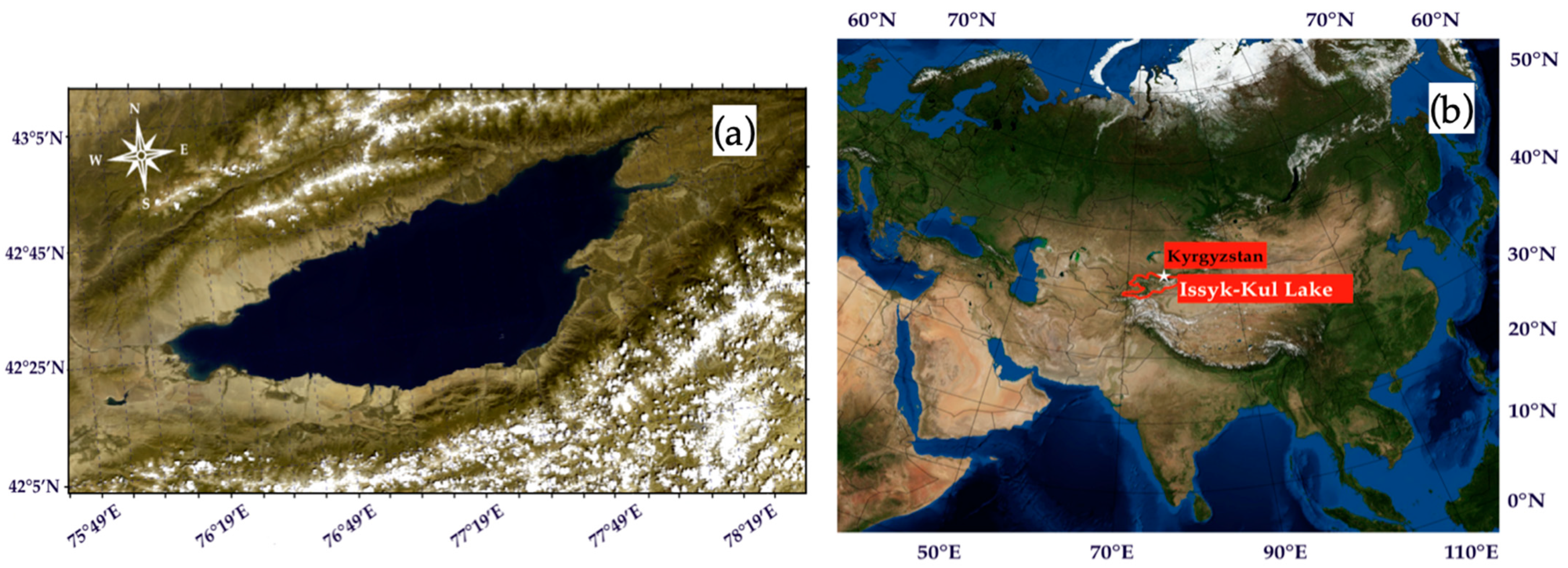
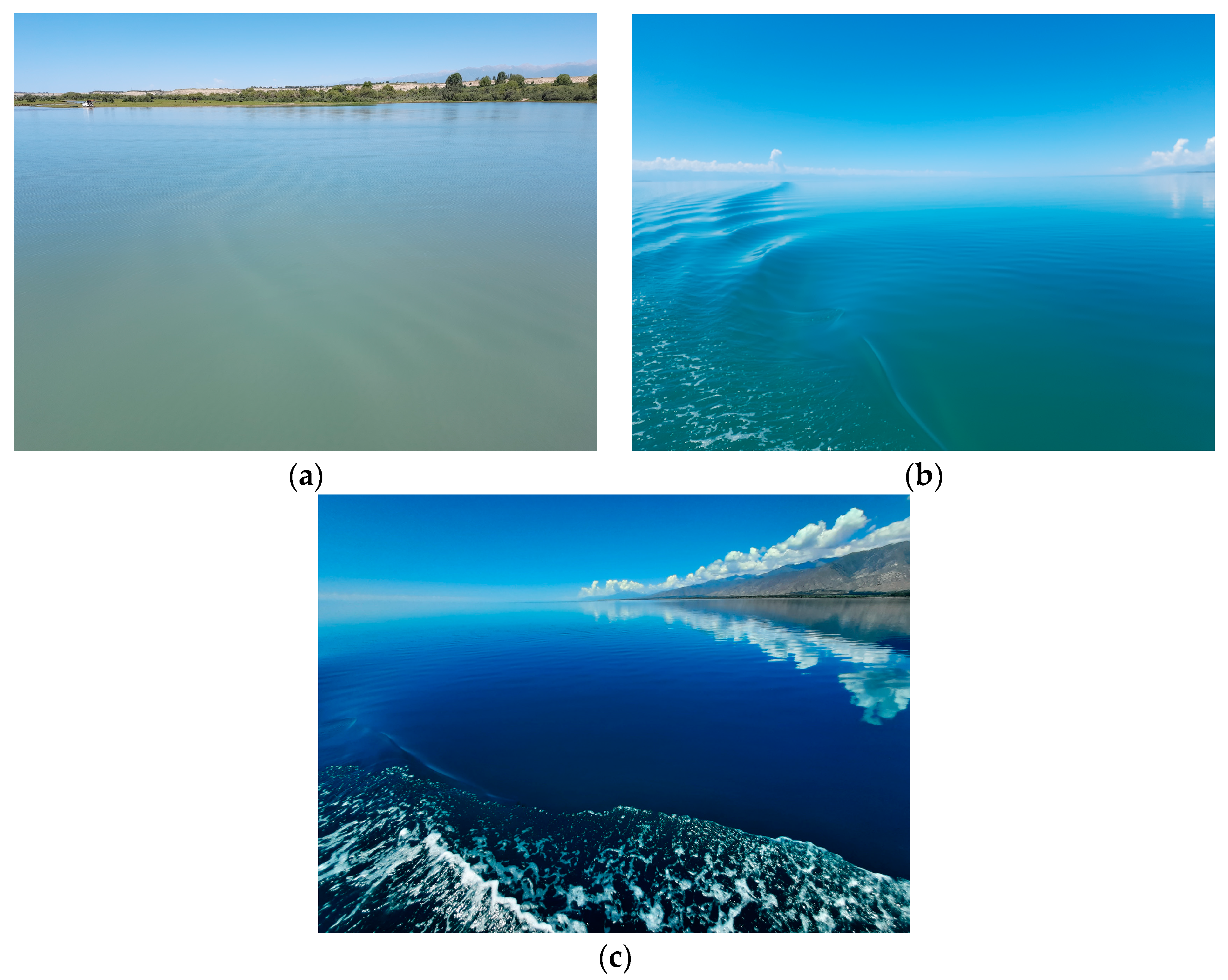
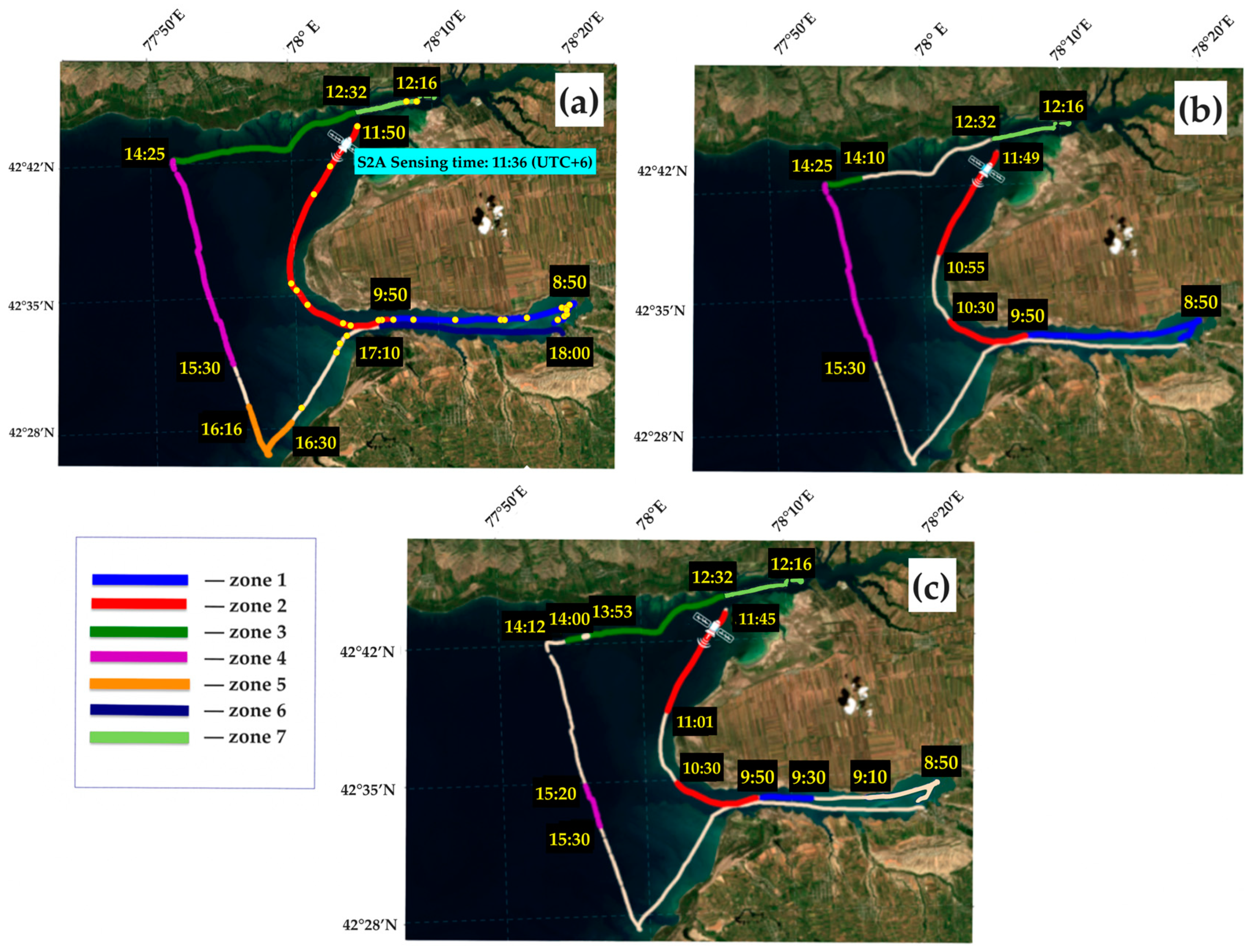
2.1. Study Region
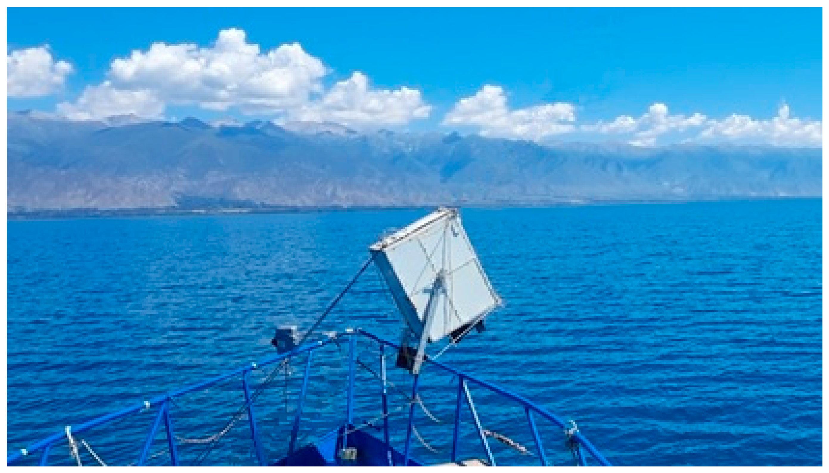
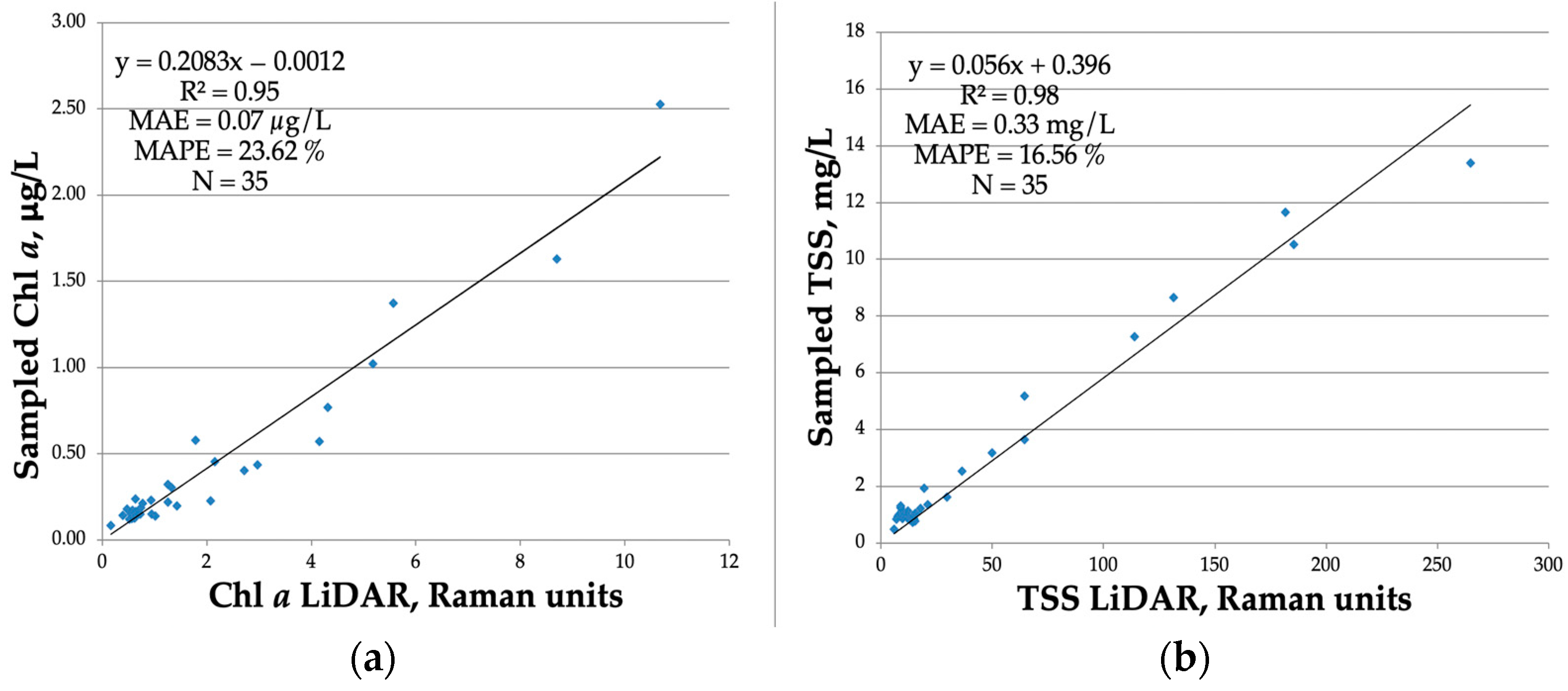
2.2. Field Measurements
2.3. Sentinel-2/MSI Imagery and Image Processing
2.3.1. Match-Ups for Satellite Validation and Spatial-Temporal Variability within a Pixel
2.3.2. Accuracy Metrics
3. Results and Discussion
3.1. Statistics of Chl a and TSS Variations
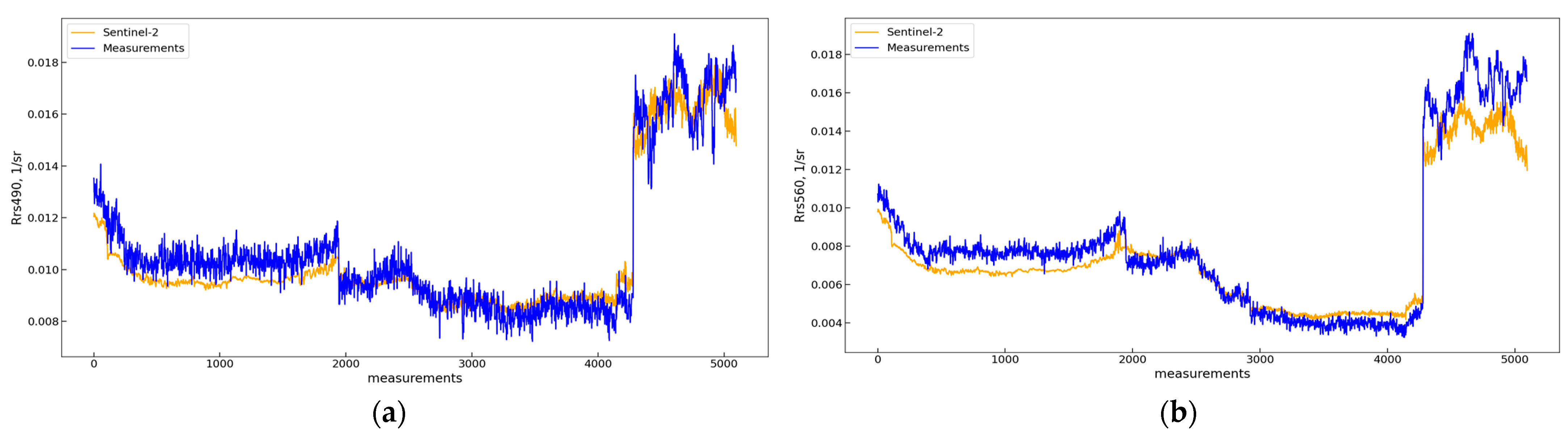
3.2. Reflectance Spectra
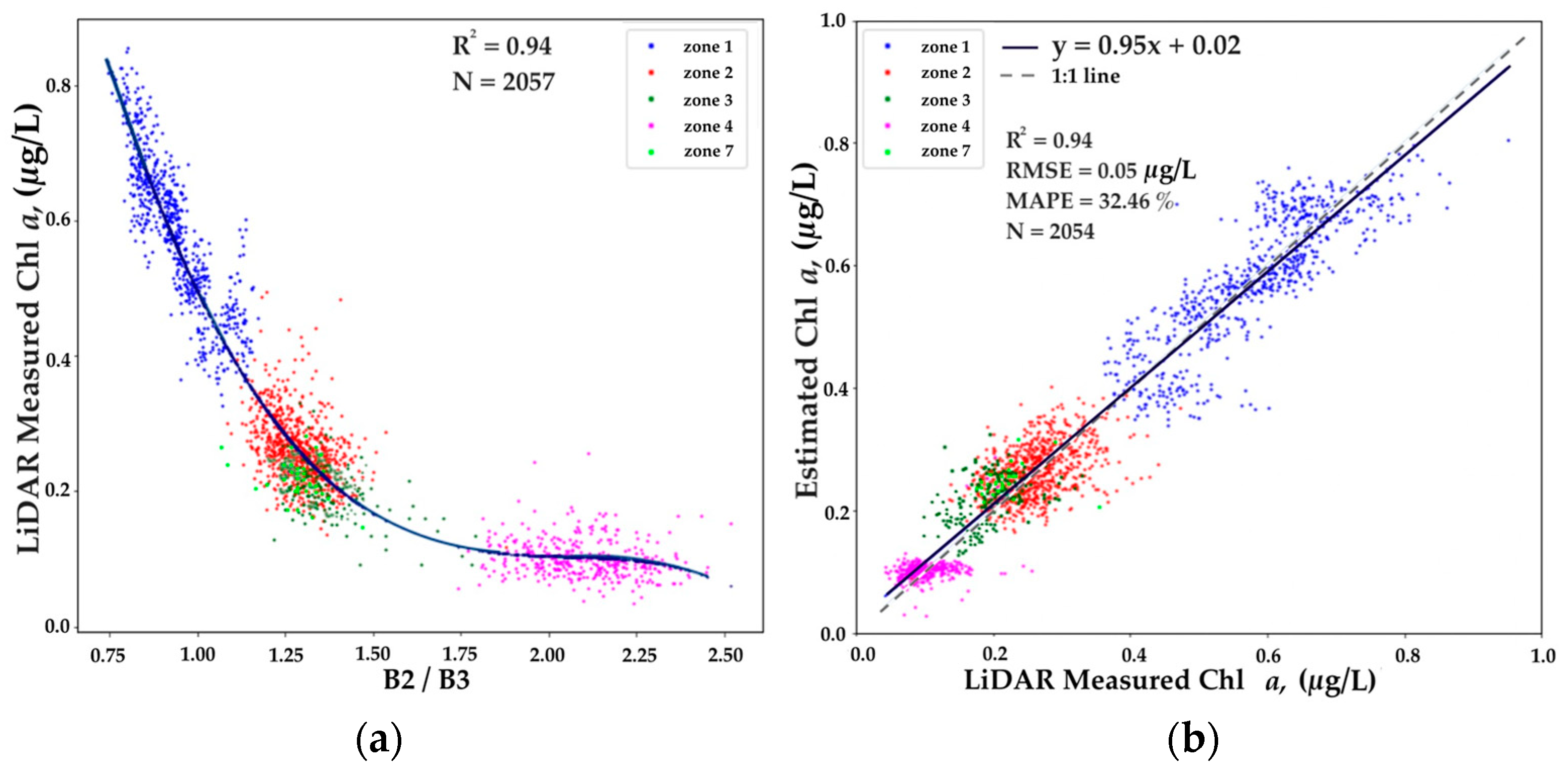
3.3. Chl a Model
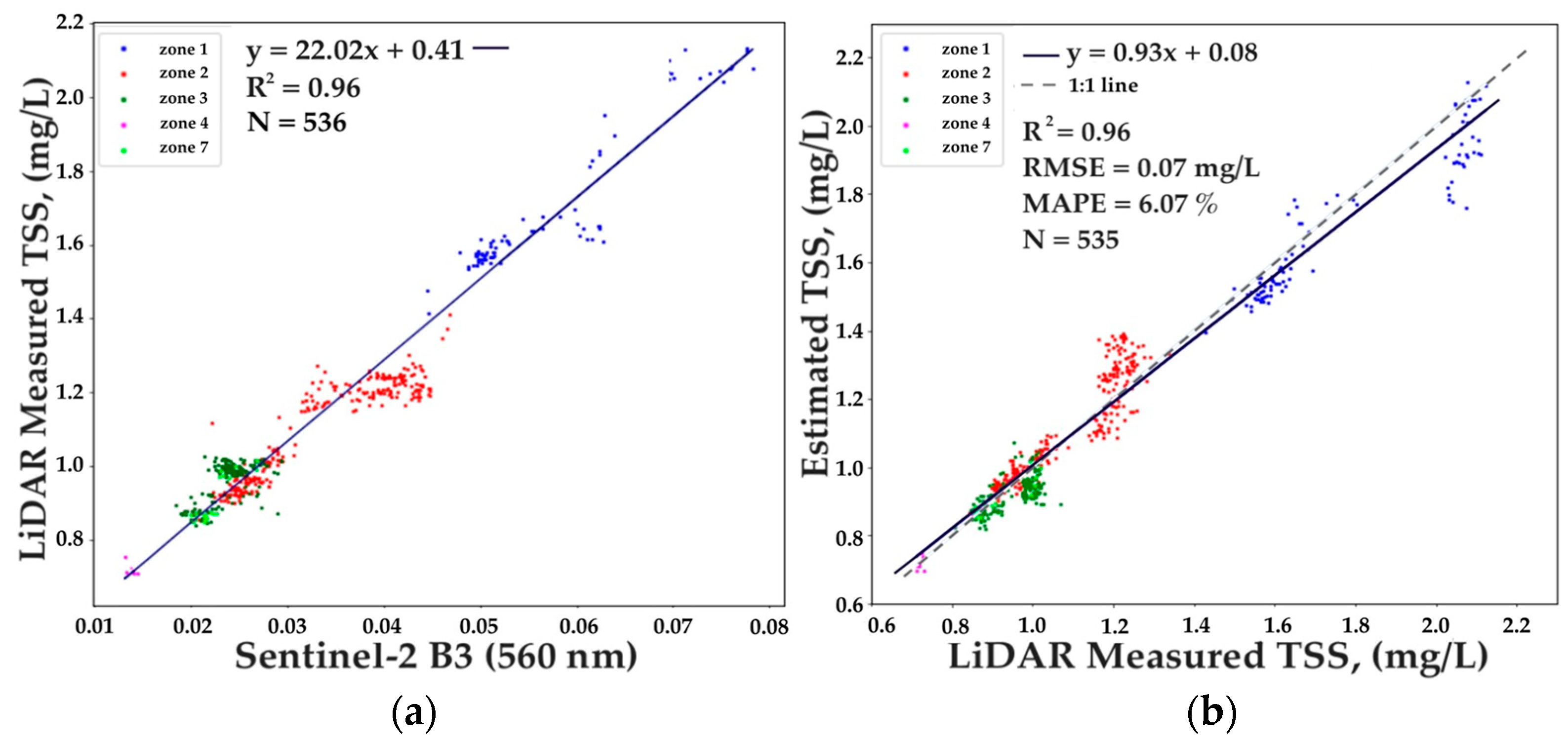
3.4. TSS Model
3.5. Comparison of Conventional and Newly Developed Bio-Optical Models of Chl a and TSS
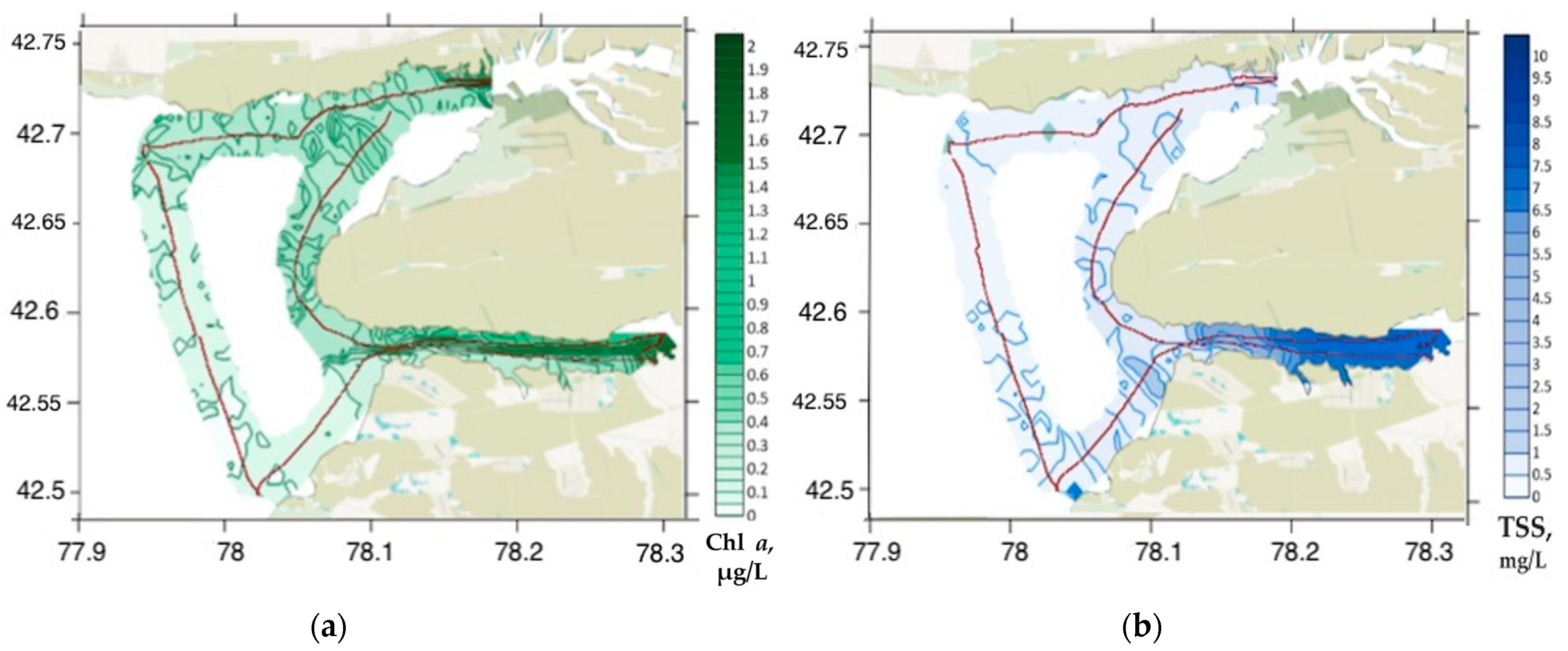
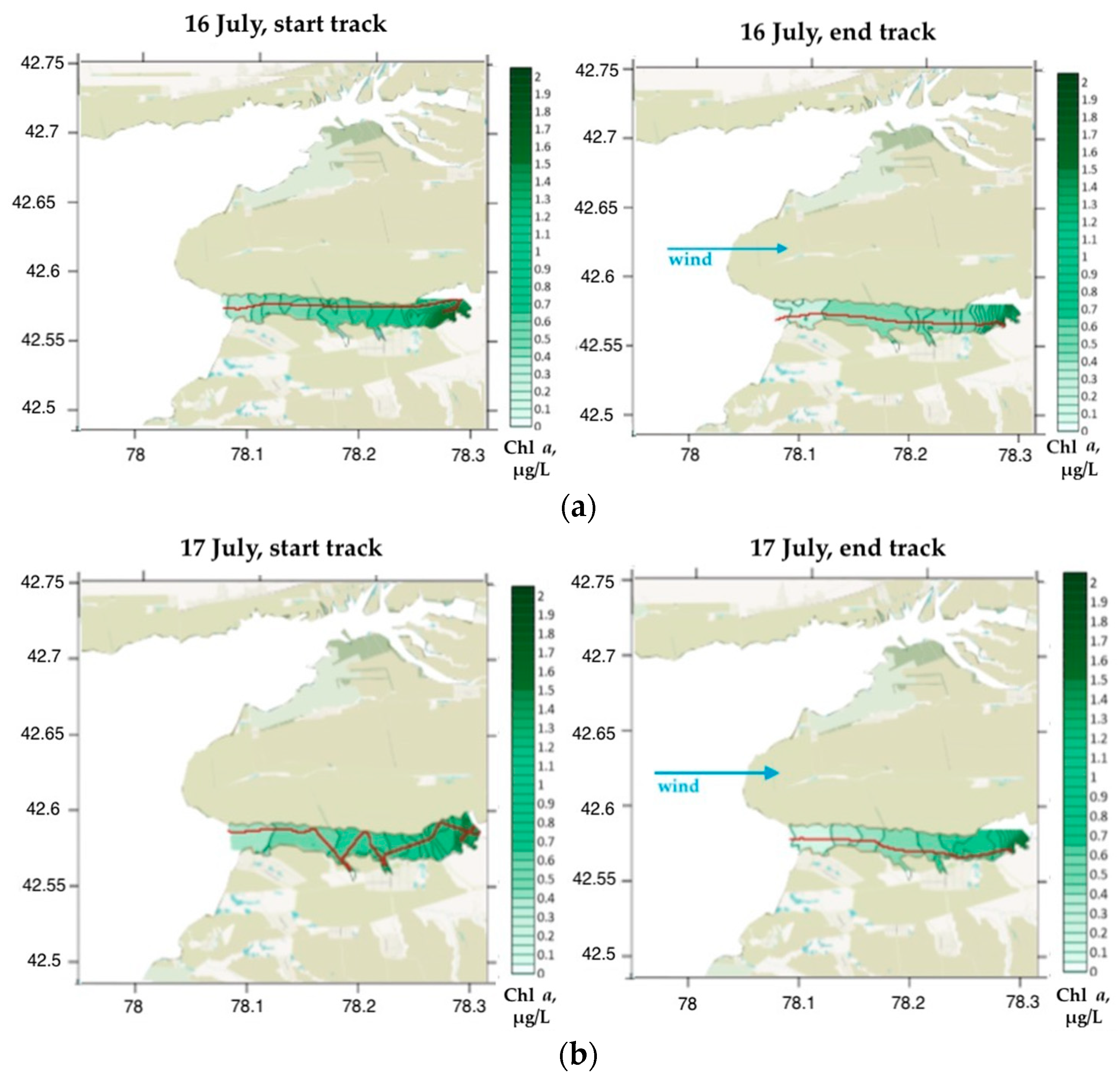
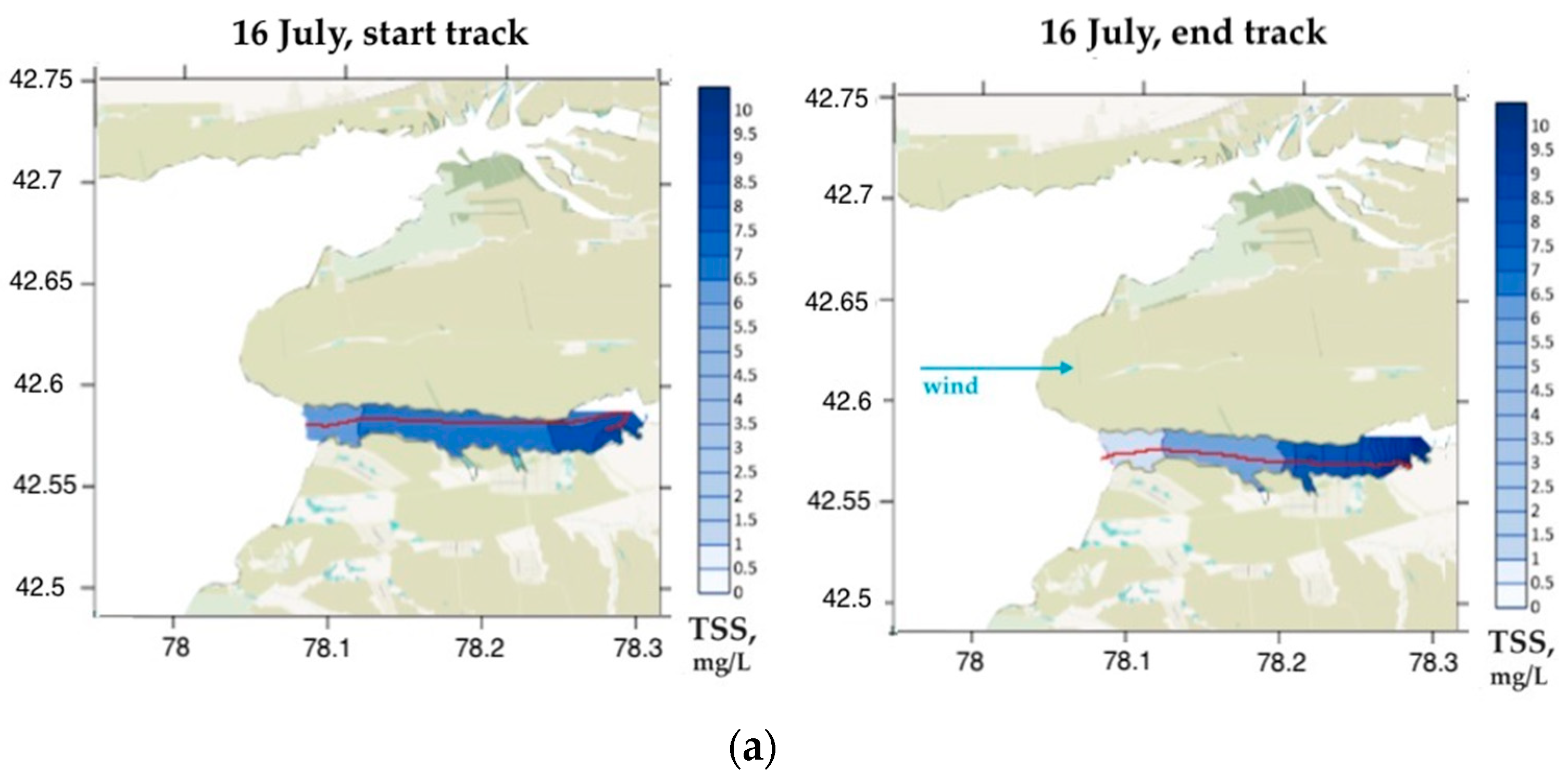
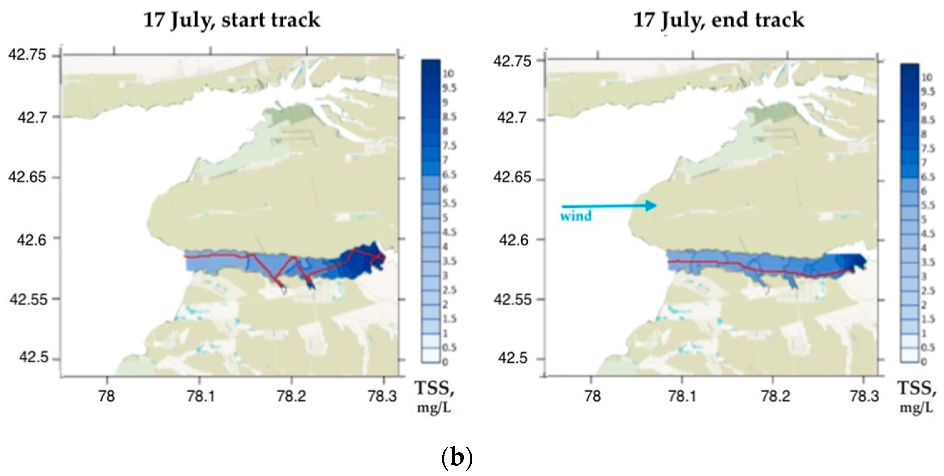
3.6. Chl a and TSS Mapping Using LIF LiDAR Data
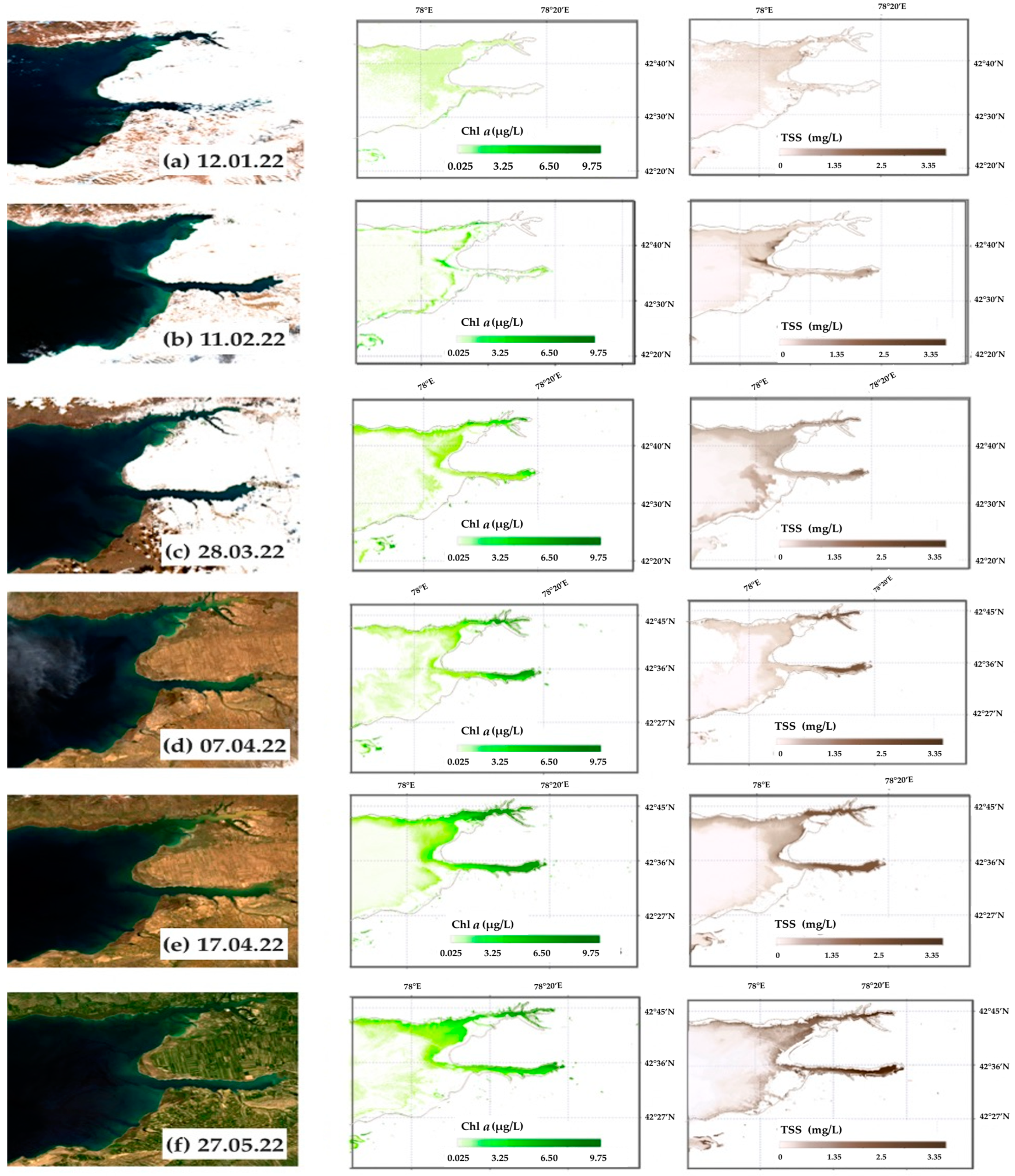
3.7. Chl a and TSS Mapping Using Sentinel-2 Data
4. Conclusions
Author Contributions
Funding
Data Availability Statement
Acknowledgments
Conflicts of Interest
Appendix A


| Metrics/Wavelength | 440 | 490 | 560 | 665 | 705 | 740 |
| Slope | 1.2444 | 0.899 | 0.7693 | 0.3461 | 0.2487 | 0.1413 |
| Intercept | −0.0058 | 0.0026 | 0.0041 | 0.0036 | 0.0038 | 0.0041 |
| R | 0.949 | 0.96 | 0.981 | 0.814 | 0.707 | 0.422 |
| RMSE | 0.0036 | 0.0026 | 0.0039 | 0.003 | 0.0029 | 0.0029 |
| bias | 0.0024 | −0.0009 | −0.0018 | 0.0008 | 0.0012 | 0.0016 |
| MAPE | 7.0 | 6.0 | 10.9 | 225.1 | 270.5 | 368.6 |
References
- Toming, K.; Kutser, T.; Laas, A.; Sepp, M.; Paavel, B.; Nõges, T. First Experiences in Mapping Lake Water Quality Parameters with Sentinel-2 MSI Imagery. Remote Sens. 2016, 8, 640. [Google Scholar] [CrossRef]
- Molkov, A.A.; Fedorov, S.V.; Pelevin, V.V.; Korchemkina, E.N. Regional Models for High-Resolution Retrieval of Chlorophyll a and TSS Concentrations in the Gorky Reservoir by Sentinel-2 Imagery. Remote Sens. 2019, 11, 1215. [Google Scholar] [CrossRef]
- Dörnhöfer, K.; Göritz, A.; Gege, P.; Pflug, B.; Oppelt, N. Water constituents and water depth retrieval from Sentinel-2a—A first evaluation in an oligotrophic lake. Remote Sens. 2016, 8, 941. [Google Scholar] [CrossRef]
- Pahlevan, N.; Smith, B.; Schalles, J.; Binding, C.; Cao, Z.; Ma, R.; Alikas, K.; Kangro, K.; Gurlin, D.; Hà, N.; et al. Seamless Retrievals of Chlorophyll-a from Sentinel-2 (MSI) and Sentinel-3 (OLCI) in Inland and Coastal Waters: A Machine-Learning Approach. Remote Sens. Environ. 2020, 240, 111604. [Google Scholar] [CrossRef]
- Palmer, S.; Hunter, P.; Lankester, T.; Hubbard, S.; Spyrakos, E.; Tyler, A.; Présing, M.; Horváth, H.; Lamb, A.; Balzter, H.; et al. Validation of Envisat MERIS Algorithms for Chlorophyll Retrieval in a Large, Turbid and Optically Complex Shallow Lake. Remote Sens. Environ. 2014, 5, 157. [Google Scholar] [CrossRef]
- Pelevin, V.; Zlinszky, A.; Khimchenko, E.; Toth, V. Ground truth data on Chlorophyll-a, chromophoric dissolved organic constituents and suspended sediment concentrations in the upper water layer as obtained by LIF LiDARat high spatial resolution. Int. J. Remote Sens. 2017, 38, 1967–1982. [Google Scholar] [CrossRef]
- Zavialov, P.; Izhitskiy, A.; Kirillin, G.; Khan, V.; Konovalov, B.; Makkaveev, P.; Pelevin, V.; Rimskiy-Korsakov, N.; Alymkulov, S.; Zhumaliev, K. New profiling and mooring records help to assess variability of Lake Issyk-Kul and reveal unknown features of its thermohaline structure. Hydrol. Earth Syst. Sci. 2018, 22, 6279–6295. [Google Scholar] [CrossRef]
- Zavyalov, P.O.; Zhumaliev, K.M.; Alymkulov, S.A.; Konovalov, B.V.; Makkaveev, P.N.; Pelevin, V.V.; Rimsky-Korsakov, N.A.; Izhitsky, A.S.; Izhitskaya, E.S. Comprehensive Studies of Lake Issyk-Kul: Part 1; Kyrgyz-Russian Slavic University: Bishkek, Kyrgyzstan, 2018; p. 194. (In Russian) [Google Scholar]
- Romanovsky, V.V. Lake Issyk-Kul as a Natural Complex; Frunze: Ilim, Russia, 1991; p. 169. (In Russian) [Google Scholar]
- Zavialov, P.O.; Pelevin, V.V.; Belyaev, N.A.; Izhitskiy, A.S.; Konovalov, B.V.; Krementskiy, V.V.; Goncharenko, I.V.; Osadchiev, A.A.; Soloviev, D.M.; Garcia, C.A.E.; et al. High resolution LiDARmeasurements reveal fine internal structure and variability of sediment-carrying coastal plume. Estuar. Coast. Shelf Sci. 2018, 205, 40–45. [Google Scholar] [CrossRef]
- Zavyalov, P.O.; Alymkulov, S.A.; Zhumaliev, K.M.; Israilova, N.A.; Konovalov, B.V.; Sapozhnikov, F.V.; Makkaveev, P.N.; Khan, V.M.; Pelevin, V.V.; Izhitsky, A.S.; et al. Comprehensive Studies of Lake Issyk-Kul: Part 2; Kyrgyz-Russian Slavic University: Bishkek, Kyrgyzstan, 2020; p. 208. (In Russian) [Google Scholar]
- Pereira-Sandoval, M.; Ruescas, A.B.; García-Jimenez, J.; Blix, K.; Delegido, J.; Moreno, J. Supervised Classifications of Optical Water Types in Spanish Inland Waters. Remote Sens. 2022, 14, 5568. [Google Scholar] [CrossRef]
- Vanderhoof, M.K.; Alexander, L.; Christensen, J.; Solvik, K.; Nieuwlandt, P.; Sagehorn, M. High-frequency time series comparison of Sentinel-1 and Sentinel-2 satellites for mapping open and vegetated water across the United States (2017–2021). Remote Sens. Environ. 2023, 288, 113498. [Google Scholar] [CrossRef] [PubMed]
- Many, G.; Escoffier, N.; Ferrari, M.; Jacquet, P.; Odermatt, D.; Mariethoz, G.; Perolo, P.; Perga, M.-E. Long-Term Spatiotemporal Variability of Whitings in Lake Geneva from Multispectral Remote Sensing and Machine Learning. Remote Sens. 2022, 14, 6175. [Google Scholar] [CrossRef]
- Balasubramanian, S.V.; Pahlevan, N.; Smith, B.; Binding, C.; Schalles, J.; Loisel, H.; Gurlin, D.; Greb, S.; Alikas, K.; Randla, M.; et al. Robust algorithm for estimating total suspended solids (TSS) in inland and nearshore coastal waters. Remote Sens. Environ. 2020, 246, 111768. [Google Scholar] [CrossRef]
- Jiang, Y.-J.; He, W.; Liu, W.-X.; Qin, N.; Ouyang, H.-L.; Wang, Q.-M.; Kong, X.-Z.; He, Q.-S.; Yang, C.; Yang, B. The seasonal and spatial variations of phytoplankton community and their correlation with environmental factors in a large eutrophic Chinese lake (Lake Chaohu). Ecol. Indic. 2014, 40, 58–67. [Google Scholar] [CrossRef]
- Wynne, T.T.; Stumpf, R.P. Spatial and temporal patterns in the seasonal distribution of toxic cyanobacteria in western Lake Erie from 2002–2014. Toxins 2015, 7, 1649–1663. [Google Scholar] [CrossRef] [PubMed]
- Hansen, C.H.; Burian, S.J.; Dennison, P.E.; Williams, G.P. Spatiotemporal Variability of Lake Water Quality in the Context of Remote Sensing Models. Remote Sens. 2017, 9, 409. [Google Scholar] [CrossRef]
- Pelevin, V.; Zavialov, P.; Konovalov, B.; Zlinszky, A.; Palmer, S.; Toth, V.; Goncharenko, I.; Khymchenko, L.; Osokina, V. Measurements with high spatial resolution of Chlorophyll-a, CDOM and total suspended constituents in coastal zones and inland water basins by the portable UFL Lidar. In Proceedings of the 35th EARSeL Symposium—European Remote Sensing: Progress, Challenges and Opportunities, Stockholm, Sweden, 15–19 June 2015. [Google Scholar]
- Hoge, F.E.; Lyon, P.E.; Swift, R.N.; Yungel, J.K.; Abbott, M.R.; Letelier, R.M.; Esaias, W.E. Validation of Terra-MODIS phytoplankton chlorophyll fluorescence line height. I. Initial airborne LiDARresults. Appl. Opt. 2003, 42, 2767–2771. [Google Scholar] [CrossRef]
- Aibulatov, N.A.; Zavialov, P.O.; Pelevin, V.V. Some Features of Self-Purification of Russian Black Sea Shoaling Waters near River Entries. Geosci. Ecol. 2008, 4, 301–310. [Google Scholar]
- Vasilescu, J.; Onciu, T.; Jugaru, L.; Belegante, L. Remote estimation of fluorescence marine components distribution. Rom. Rep. Phys. 2009, 61, 721–729. [Google Scholar]
- Cisek, M.; Colao, F.; Demetrio, E.; Di Cicco, A.; Drozdowska, V.; Goszczko, I.; Fiorani, L.; Lazic, V.; Okladnikov, I.G.; Palucci, A.; et al. Remote and local monitoring of dissolved and suspended fluorescent organic matter off the Svalbard. J. Optoelectron. Adv. Mater. 2010, 12, 1604. [Google Scholar]
- Pelevin, V.V.; Zavjalov, P.O.; Belyaev, N.A.; Konovalov, B.V.; Kravchishina, M.D.; Mosharov, S.A. Spatial variability of concentrations of chlorophyll a, dissolved organic matter and suspended particles in the surface layer of the Kara Sea in September 2011 from LiDAR data. Oceanology 2017, 57, 165–173. [Google Scholar] [CrossRef]
- Drozdowska, V. The LiDAR investigation of the upper water layer fluorescence spectra of the Baltic Sea. Eur. Phys. J. Spec. Top. 2007, 144, 141–145. [Google Scholar] [CrossRef]
- Barbini, R.; Colao, F.; Fantoni, R.; L Fiorani, L.; Palucci, A. Remote sensing of the Southern Ocean: Techniques and results. J. Optoelectron. Adv. Mater. 2001, 3, 817–830. [Google Scholar]
- Zavialov, P.O.; Kopelevich, O.V.; Kremenetskiy, V.V.; Pelevin, V.V.; Grabovskiy, A.B.; Gureev, B.A.; Grigoriev, A.V.; Peresypkin, V.I.; Ding, C.F.; Hsu, M.H. A joint Russian-Taiwanese expedition at the shelf of the South China Sea: Searching for manifestations of groundwater discharge to the ocean. Oceanology 2010, 50, 618–622. [Google Scholar] [CrossRef]
- Zavialov, P.O.; Barbanova, E.S.; Pelevin, V.V.; Osadchiev, A.A. Estimating the deposition of river-borne suspended matter from the joint analysis of suspension concentration and salinity. Oceanology 2015, 55, 832–836. [Google Scholar] [CrossRef]
- Collister, B.L.; Zimmerman, R.C.; Sukenik, C.I.; Hill, V.J.; Balch, W.M. Remote sensing of optical characteristics and particle distributions of the upper ocean using shipboard lidar. Remote Sens. Environ. 2018, 215, 85–96. [Google Scholar] [CrossRef]
- Palmer, S.C.J.; Pelevin, V.V.; Goncharenko, I.; Kovács, A.W.; Zlinszky, A.; Présing, M.; Horváth, H.; Nicolás-Perea, V.; Balzter, H.; Tóth, V.R. Ultraviolet fluorescence LiDAR(UFL) as a measurement tool for water quality parameters in turbid lake conditions. Remote Sens. 2013, 5, 4405–4422. [Google Scholar] [CrossRef]
- Chen, P.; Pan, D.; Wang, T.; Mao, Z.; Zhang, Y. Coastal and inland water monitoring using a portable hyperspectral laser fluorometer. Mar. Pollut. Bull. 2017, 119, 153–161. [Google Scholar] [CrossRef] [PubMed]
- Duan, Z.; Li, Y.; Wang, J.; Zhao, G.; Svanberg, S. Aquatic environment monitoring using a drone-based fluorosensor. Appl. Phys. B 2019, 125, 108. [Google Scholar] [CrossRef]
- Fiorani, L.; Barbini, R.; Colao, F.; De Dominicis, L.; Fantoni, R.; Palucci, A.; Artamonov, E.S. Combination of lidar, MODIS and SEAWIFS sensors for simultaneous chlorophyll monitoring. EARSeL eProc. 2004, 3, 8–17. [Google Scholar]
- Fiorani, L.; Fantoni, R.; Lazzara, L.; Nardello, I.; Okladnikov, I.G.; Palucci, A. LiDAR calibration of satellite sensed CDOM in the Southern Ocean. EARSeL eProc. 2006, 5, 89–99. [Google Scholar]
- Li, X.; Zhao, C.; Ma, Y.; Liu, Z. Field experiments of multi-channel oceanographic fluorescence LiDAR for oil spill and chlorophyll-a detection. J. Ocean. Univ. China 2014, 13, 597–603. [Google Scholar] [CrossRef]
- Molkov, A.A.; Pelevin, V.V.; Korchemkina, E.N. Approach of non-station-based in situ measurements for high resolution satellite remote sensing of productive and highly changeable inland waters. Fundam. Appl. Hydrophys. 2020, 13, 60–67. [Google Scholar] [CrossRef]
- Mueller, J.L.; Pietras, C.; Hooker, S.B.; Austin, R.W.; Miller, M.; Knobelspiesse, K.D.; Frouin, R.; Holben, B.; Voss, K. Ocean Optics Protocols for Satellite Ocean Color Sensor Validation, Revision 4, Volume II: Instrument Specifications, Characterization and Calibration; NASA/TM-2003-21621/Rev-Vol II; Goddard Space Flight Space Center: Greenbelt, MD, USA, 2003; pp. 1–56.
- SCOR-UNESCO. Report of SCOR-UNESCO working group 17 on determination of photosynthetic pigments in Sea Water. In Monograph of Oceanography Methodology; UNESCO: Paris, France, 1966; Volume 1, pp. 9–18. [Google Scholar]
- Konovalov, B.V.; Kravchishina, M.D.; Belyaev, N.A.; Novigatsky, A.N. Determination of the concentration of mineral particles and suspended organic substance based on their spectral absorption. Oceanology 2014, 54, 660–667. [Google Scholar] [CrossRef]
- Mueller, J.L.; Bidigare, R.R.; Trees, C.; Balch, W.M.; Dore, J.; Drapeau, D.T.; Karl, D.; Van Heukelem, L.; Perl, J. Ocean Optics Protocols for Satellite Ocean Color Sensor Validation, Revision 5, Volume 5: Biogeochemical and Bio-Optical Measurements and Data Analysis Protocols; Goddard Space Flight Space Center: Greenbelt, MD, USA, 2003; pp. 5–24. [Google Scholar]
- Mobley, C.D. Estimation of the remote sensing reflectance from above–water methods. Appl. Opt. 1999, 38, 7442–7455. [Google Scholar] [CrossRef] [PubMed]
- Dierssen, H.M.; Vandermeulen, R.A.; Barnes, B.B.; Castagna, A.; Knaeps, E.; Vanhellemont, Q. QWIP: A Quantitative Metric for Quality Control of Aquatic Reflectance Spectral Shape Using the Apparent Visible Wavelength. Front. Remote Sens. 2022, 3, 869611. [Google Scholar] [CrossRef]
- Spyrakos, E.; O’Donnell, R.; Hunter, P.D.; Miller, C.; Scott, M.; Simis, S.G.H.; Neil, C.; Barbosa, C.C.F.; Binding, C.E.; Bradt, S.; et al. Optical types of inland and coastal waters. Limnol. Oceanogr. 2018, 63, 846–870. [Google Scholar] [CrossRef]
- Franz, B.A.; Bailey, S.W.; Kuring, N.; Werdell, P.J. Ocean color measurements with the Operational Land Imager on Landsat-8: Implementation and evaluation in SeaDAS. J. Appl. Remote Sensing. 2015, 9, 096070. [Google Scholar] [CrossRef]
- Nechad, B.; Ruddick, K.G.; Park, Y. Calibration and Validation of a Generic Multisensor Algorithm for Mapping of Total Suspended Matter in Turbid Waters. Remote Sens. Environ. 2010, 114, 854–866. [Google Scholar] [CrossRef]
- Odermatt, D.; Gitelson, A.; Brando, V.E.; Schaepman, M. Review of Constituent Retrieval in Optically Deep and Complex Waters from Satellite Imagery. Remote Sens. Environ. 2012, 118, 116–126. [Google Scholar] [CrossRef]
- Morel, A.; Huot, Y.; Gentili, B.; Werdell, P.J.; Hooker, S.B.; Franz, B.A. Examining the consistency of products derived from various ocean color sensors in open ocean (Case 1) waters in the perspective of a multi-sensor approach. Remote Sens. Environ. 2007, 111, 69–88. [Google Scholar] [CrossRef]


| Parameter | N | Min | Max | Mean | Median | STD |
|---|---|---|---|---|---|---|
| Chl a (µg/L) | 4111 | 0.032 | 0.952 | 0.328 | 0.293 | 0.201 |
| TSS (mg/L) | 1071 | 0.707 | 2.133 | 1.155 | 1.012 | 0.324 |
| Dataset | N | Min | Max | Mean | Median | STD |
|---|---|---|---|---|---|---|
| Calibration | 2057 | 0.036 | 0.952 | 0.328 | 0.293 | 0.202 |
| Validation | 2054 | 0.032 | 0.864 | 0.327 | 0.291 | 0.199 |
| All | 4111 | 0.032 | 0.952 | 0.328 | 0.292 | 0.201 |
| Dataset | N | Min | Max | Mean | Median | STD |
|---|---|---|---|---|---|---|
| Calibration | 536 | 0.707 | 2.131 | 1.154 | 1.010 | 0.324 |
| Validation | 535 | 0.712 | 2.133 | 1.155 | 1.012 | 0.323 |
| All | 1071 | 0.707 | 2.133 | 1.155 | 1.012 | 0.324 |
| Sentinel-2 Image | Chl a Maps | TSS Maps |
|---|---|---|
 | ||
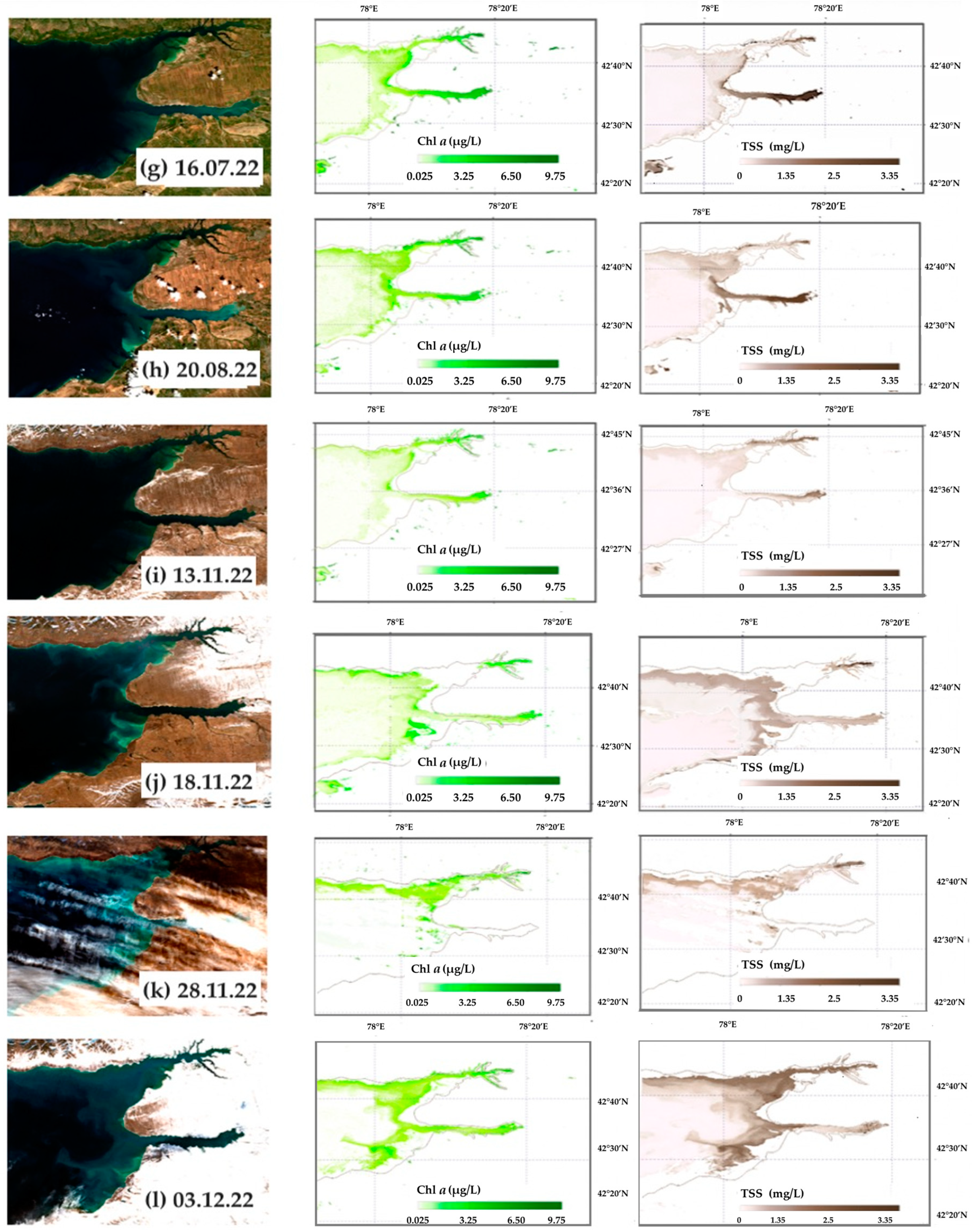 | ||
| Image | Date | Max Chl a (µg/L) | Min Chl a (µg/L) | Max TSS (mg/L) | Min TSS (mg/L) |
|---|---|---|---|---|---|
| a | 12 January 2022 | 2.2 | 0.01 | 2.2 | 0.11 |
| b | 11 February 2022 | 3.5 | 0.01 | 2.8 | 0.11 |
| c | 28 March 2022 | 5.0 | 0.01 | 2.1 | 0.12 |
| d | 7 April 2022 | 6.5 | 0.01 | 3.6 | 0.10 |
| e | 17 April 2022 | 6.6 | 0.01 | 4.0 | 0.11 |
| f | 27 May 2022 | 6.6 | 0.01 | 3.4 | 0.10 |
| g | 16 July 2022 | 6.2 | 0.01 | 3.6 | 0.12 |
| h | 20 August 2022 | 6.2 | 0.02 | 3.2 | 0.11 |
| i | 13 November 2022 | 2.2 | 0.01 | 2.1 | 0.10 |
| j | 18 November 2022 | 2.3 | 0.02 | 2.4 | 0.10 |
| k | 28 November 2022 | 2.4 | 0.01 | 2.0 | 0.11 |
| l | 3 December 2022 | 2.3 | 0.01 | 2.2 | 0.11 |
Disclaimer/Publisher’s Note: The statements, opinions and data contained in all publications are solely those of the individual author(s) and contributor(s) and not of MDPI and/or the editor(s). MDPI and/or the editor(s) disclaim responsibility for any injury to people or property resulting from any ideas, methods, instructions or products referred to in the content. |
© 2023 by the authors. Licensee MDPI, Basel, Switzerland. This article is an open access article distributed under the terms and conditions of the Creative Commons Attribution (CC BY) license (https://creativecommons.org/licenses/by/4.0/).
Share and Cite
Pelevin, V.; Koltsova, E.; Molkov, A.; Fedorov, S.; Alymkulov, S.; Konovalov, B.; Alymkulova, M.; Jumaliev, K. Regional Models for Sentinel-2/MSI Imagery of Chlorophyll a and TSS, Obtained for Oligotrophic Issyk-Kul Lake Using High-Resolution LIF LiDAR Data. Remote Sens. 2023, 15, 4443. https://doi.org/10.3390/rs15184443
Pelevin V, Koltsova E, Molkov A, Fedorov S, Alymkulov S, Konovalov B, Alymkulova M, Jumaliev K. Regional Models for Sentinel-2/MSI Imagery of Chlorophyll a and TSS, Obtained for Oligotrophic Issyk-Kul Lake Using High-Resolution LIF LiDAR Data. Remote Sensing. 2023; 15(18):4443. https://doi.org/10.3390/rs15184443
Chicago/Turabian StylePelevin, Vadim, Ekaterina Koltsova, Aleksandr Molkov, Sergei Fedorov, Salmor Alymkulov, Boris Konovalov, Mairam Alymkulova, and Kubanychbek Jumaliev. 2023. "Regional Models for Sentinel-2/MSI Imagery of Chlorophyll a and TSS, Obtained for Oligotrophic Issyk-Kul Lake Using High-Resolution LIF LiDAR Data" Remote Sensing 15, no. 18: 4443. https://doi.org/10.3390/rs15184443