Abstract
To address the problem of the expensive and time-consuming annotation of high-resolution remote sensing images (HRRSIs), scholars have proposed cross-domain scene classification models, which can utilize learned knowledge to classify unlabeled data samples. Due to the significant distribution difference between a source domain (training sample set) and a target domain (test sample set), scholars have proposed domain adaptation models based on deep learning to reduce the above differences. However, the existing models have the following shortcomings: (1) insufficient learning of feature information, resulting in feature loss and restricting the spatial extent of domain-invariant features; (2) models easily focus on background feature information, resulting in negative transfer; (3) the relationship between the marginal distribution and the conditional distribution is not fully considered, and the weight parameters between them are manually set, which is time-consuming and may fall into local optimum. To address the above problems, this study proposes a novel remote sensing cross-domain scene classification model based on Lie group spatial attention and adaptive multi-feature distribution. Concretely, the model first introduces Lie group feature learning and maps the samples to the Lie group manifold space. By learning features of different levels and different scales and feature fusion, richer features are obtained, and the spatial scope of domain-invariant features is expanded. In addition, we also design an attention mechanism based on dynamic feature fusion alignment, which effectively enhances the weight of key regions and dynamically balances the importance between marginal and conditional distributions. Extensive experiments are conducted on three publicly available and challenging datasets, and the experimental results show the advantages of our proposed method over other state-of-the-art deep domain adaptation methods.
1. Introduction
In recent years, with the rapid development of remote sensing image sensor technology, the data volume and spatial resolution of high-resolution remote sensing images (HRRSIs) have been greatly improved [1,2,3,4]. However, the types of remote sensing image sensors, imaging and illumination conditions, shooting heights, and angles have led to huge differences in the distribution of HRRSI [5,6,7]. Due to the different distributions of HRRSI, the generalization ability of a trained model to be applied to other new data samples is limited. How to improve the generalization ability of models under different distributed datasets has become a significant issue in current research [8,9,10].
To effectively alleviate the problem of the weak generalization ability of a model, scholars have proposed a cross-domain scene classification model. This model mainly classifies label-sparse data (target domain) based on the knowledge learned from label-rich data (source domain), where the data in the source and target domains come from different distributions [11,12]. The domain adaptation method is one of the most widely used methods in cross-domain scene classification models [13,14]. This method maps different scenes to a common feature space [15] and assumes that the source domain and the target domain share the same category space but have different data probability distributions (domain offset) [13,16]. However, in practical application scenarios, it is difficult to find a source domain that can cover all categories of the target domain [17].
The most straightforward way to effectively alleviate domain offset is to transform the source domain and the target domain so that the different data distributions are closer together. According to the characteristics of data distribution, the method mainly includes (1) conditional distribution adaptation [18]; (2) marginal distribution adaptation [19,20]; and (3) joint distribution adaptation [21]. Othman et al. [13] proposed small-batch gradient-based dynamic sample optimization to reduce the difference between marginal and conditional distributions. Adversarial learning is also a common method of domain adaptation, which mainly reduces domain offset through a minimax game between the generator and the discriminator [22]. Shen et al. [23] proposed adversarial learning based on Wasserstein distance to learn domain-invariant features. Yu et al. [24] proposed an adaptation model based on dynamic adversarial learning, which utilizes A-distance to set the weights of marginal and conditional distributions.
The successful model mentioned above provides us with a sufficient theoretical basis for our research and has achieved impressive performance. However, for the study of remote sensing cross-domain scene classification, the above models still face the following challenges:
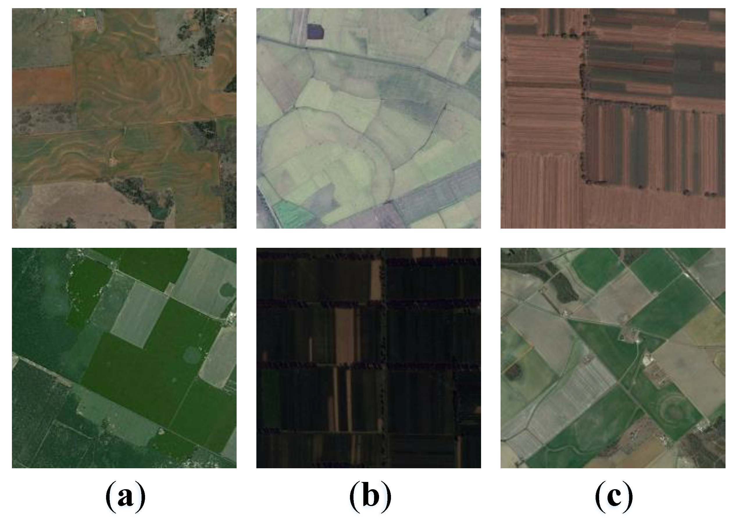
- As shown in Figure 1, due to the diversity of HRRSI generated by factors such as different heights, scales, seasons, and multiple sensors, it is difficult for the characterization of features of a certain layer (such as high-level semantic features) to cover all features in HRRSI. In other words, most existing models are mainly based on the feature information of a certain layer (such as high-level semantic features). It is difficult to capture all the feature information in HRRSI, so only some domain-invariant features may be learned.
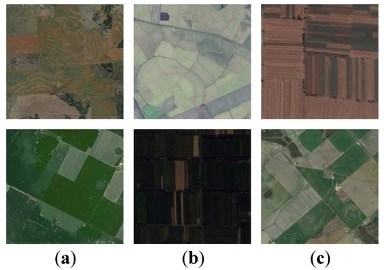 Figure 1. HRRSIs generated by some factors such as different scales, heights, seasons, and sensors are enumerated in (a–c). The samples from the AID datasets.
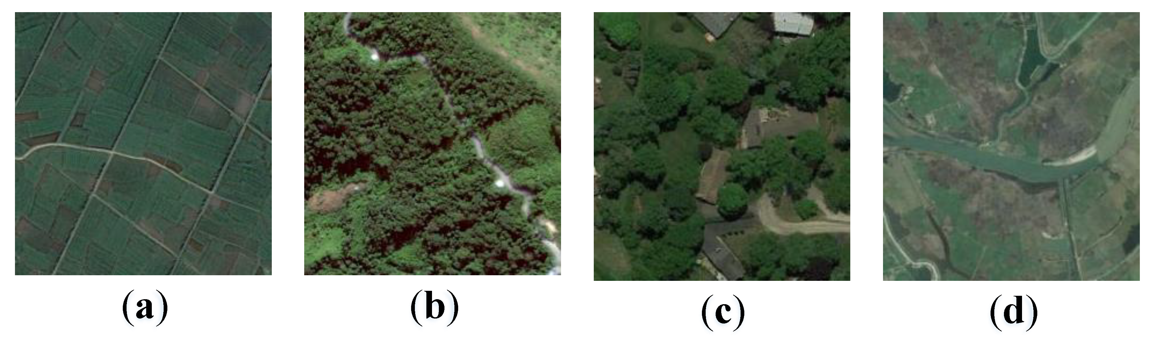
 - As shown in Figure 2, in some scenes, such as residential and river scenes, most of the existing models experience difficulty in enhancing the weight of key regions, easily focus on backgrounds, and cause negative transfer.
 Figure 2. Different scenes have different foreground proportions, such as (a) farmland, (b) forest, (c) medium residential area, and (d) rivers. Samples are from the AID datasets and NWPU-RESISC45 datasets.
 - Most existing models treat marginal distribution and conditional distribution as equally important and do not distinguish between them. In fact, the above view has been shown to be one-sided and insufficient [24]. Although some scholars have realized this problem, most of their proposed methods are based on manual methods to set the parameters of the above distribution, which may fall into local optimum. In addition, some models also align both local and global features to obtain better results, but the need to manually adjust the weights of the above two parts increases the computational difficulty and time consumption.
To address these challenges, we proposed a novel remote sensing cross-domain scene classification model based on Lie group spatial attention and adaptive multi-feature distribution. This model fully considers the representation of multi-feature spaces and expands the space of domain-invariant features. The attention mechanism in the model effectively enhances the weight of key regions; suppresses the weight of irrelevant features, such as backgrounds; and dynamically adjusts the parameters of marginal distribution and conditional distribution.
The main contributions of this study are as follows:
- To address the problem that limited feature representation cannot effectively learn sufficient features in HRRSI, we propose a multi-feature space representation module based on Lie group space, which projects HRRSIs into Lie group space and extracts features of different levels (low-level, middle-level, and high-level features) and different scales, effectively enhancing the spatial ability of domain-invariant features.
- To address the problem of negative transfer, we design an attention mechanism based on dynamic feature fusion alignment, which effectively enhances the weight of key regions, makes domain-invariant features more adaptable and transferable, and further enhances the robustness of the model.
- To address the imbalance between the relative importance of marginal distribution and conditional distribution and the problem that manual parameter setting may lead to local optimization, the proposed method takes into account the importance of the above two distributions and dynamically adjusts the parameters, effectively solving the problem of manual parameter setting and further improving the reliability of the model.
2. Method
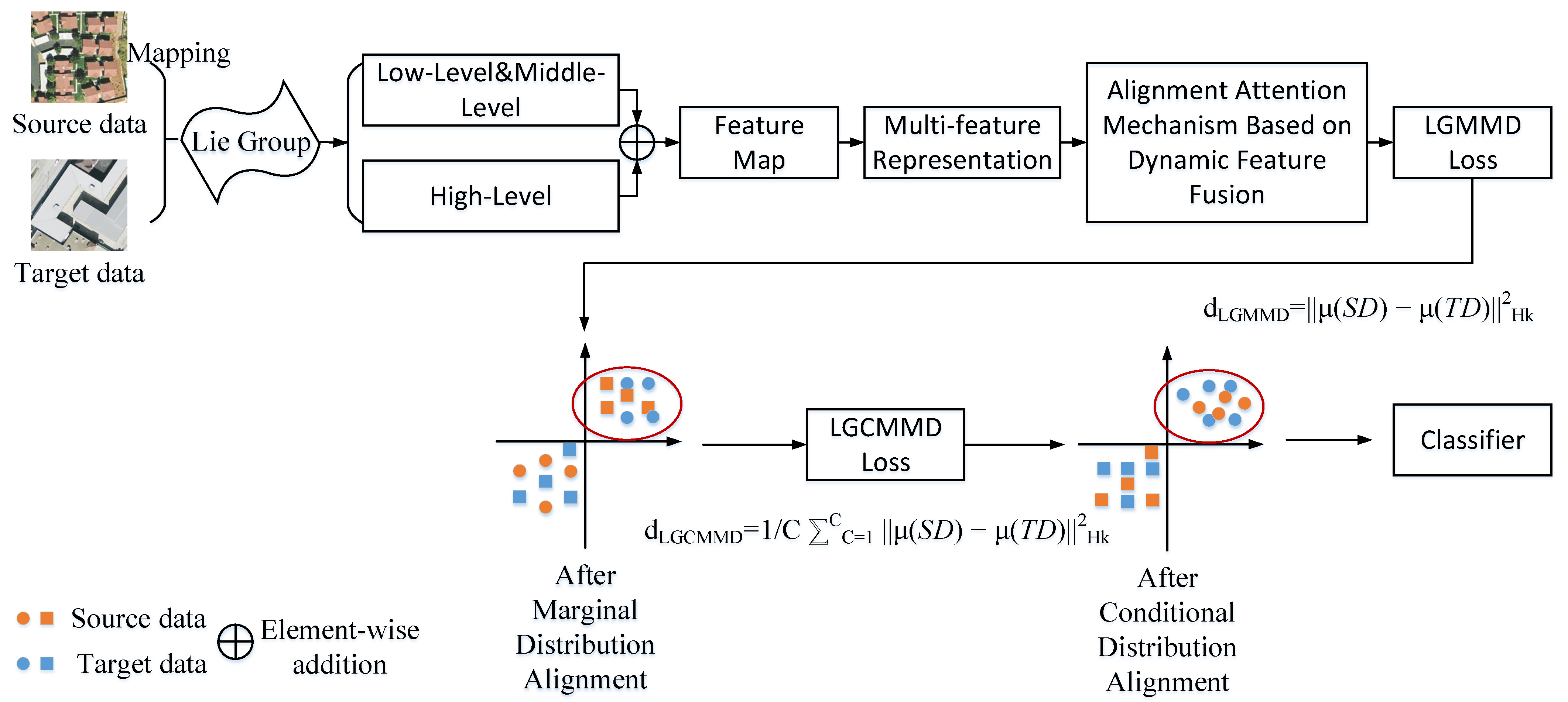
As shown in Figure 3, this section will introduce our proposed model in detail from several aspects, such as problem description, domain feature extraction, attention mechanism, and dynamic setting parameters.
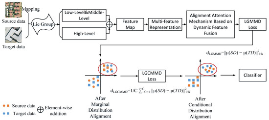
Figure 3.
Architecture of our proposed model. The model includes feature extraction modules (low-level, middle-level, and high-level features), attention mechanisms, and corresponding loss functions (LGMMD, LGCMMD).
2.1. Problem Description
represents the source domain containing -labeled samples, where represents the ith sample and represents its corresponding category information. represents the target domain containing -unlabeled samples, where represents the ith sample and represents its corresponding unknown category information. The category space and feature space of the source and target domains are the same, i.e., and , but their marginal probability distribution and conditional probability distribution are different, i.e., and . The goal of our model is to reduce the differences between the source and target domains by learning domain-invariant features in the source domain data samples.
2.2. Domain Feature Extractor
This subsection mainly includes two modules: Lie group feature learning and multi-feature representation.
2.2.1. Lie Group Feature Learning
In our previous research, we proposed Lie group feature learning [1,2,3,4]. In addition, we also draw on some approaches in the literature [25,26]. As shown in Figure 3, the previously proposed method was used in this study to extract and learn the low-level and middle-level features of the data sample samples.
Firstly, the sample is mapped to the manifold space of the Lie group to obtain the data sample of Lie group space:
where represents the data sample of the class in the dataset, and represents the data sample of class on the Lie group space.
Then, we perform feature extraction on the data samples on the Lie group space, as follows:
Among them, the first eight features mainly extract some basic features, such as coordinates and colors. Through previous research, we found that although there are differences in the shapes and sizes of the target objects, their positions are similar. In addition to target coordinate features, color features are also an important feature, such as forest scenes. At the same time, we consider the influence of different illuminations and add Y, , and features to further enhance the representation ability of the low-level features. The latter three features mainly extract middle-level features. For example, mainly focuses on the texture and detail feature information in the scene, mainly has the advantage of being invariant to monotony illumination, can simulate the single-cell receptive field of the cerebral cortex and extract the spatial orientation and other information in the scene. The content related to Lie group machine learning can be referred to in our previous research [1,2,3,4,27,28,29].
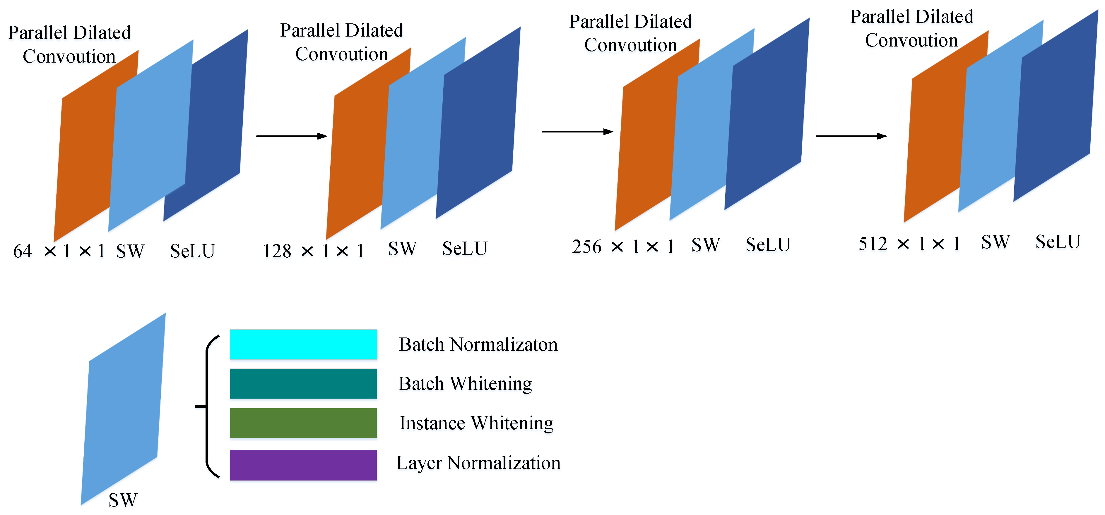
In terms of high-level feature learning, the approach shown in Figure 4 is utilized. The approach consists of four parallel dilated convolution modules, each of which is followed by switchable whitening (SW) and scaled exponential linear unit (SeLU) activation functions. The reason why traditional convolution is not used in this subsection is that, in previous research [1], we found that parallel dilated convolution can effectively expand the receptive field and learn more semantic information compared with traditional convolution, and the number of parameters is small. For details, please refer to our previous research [1]. The SW [30] method includes a variety of normalization and whitening methods, among which the whitening method can effectively reduce the pixel-to-pixel correlation of HRRSI, which is conducive to feature alignment. The SW used in this study includes batch normalization (BN), batch whitening (BW), instance whitening (IW), and layer normalization (LN), which can extract more discriminative features. In addition, in a previous study [1], we also found that the traditional rectified linear unit (ReLU) activation function directly reduces to zero in a negative semi-axis region, which may lead to the disappearance of the potential gradient in the model training phase. Therefore, we adopted the SeLU activation function based on a previous study.
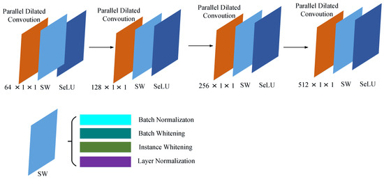
Figure 4.
High-level feature learning. The module contains parallel dilated convolution, SW operations, and SeLU activation functions.
2.2.2. Multi-Feature Representation
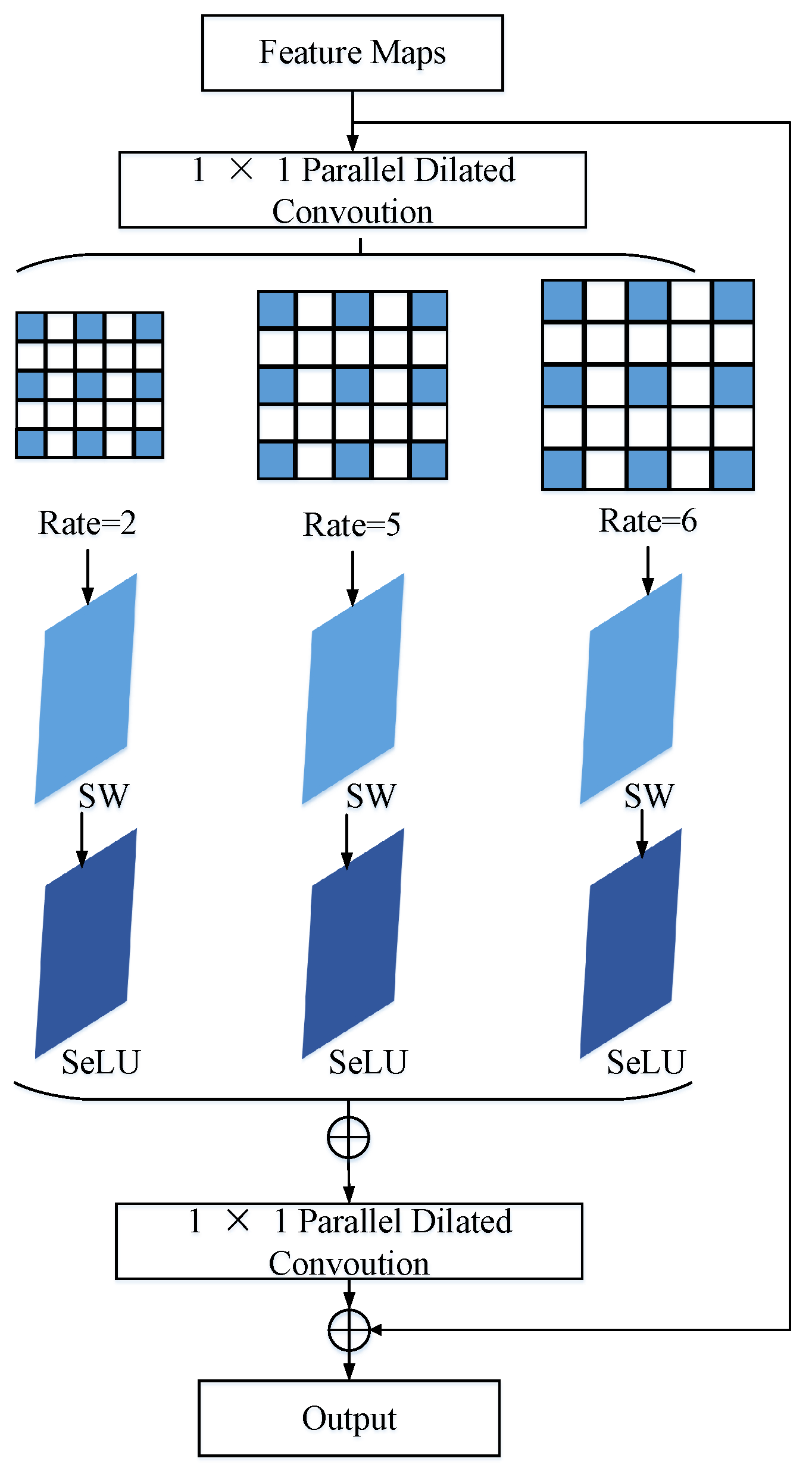
In traditional models, fixed-size convolutions are usually concatenated so that the receptive field of the obtained feature map is small, and the key feature information in HRRSI may be lost. To address this problem, in previous research [4], we proposed the multidilation pooling module, which contains four branches: the first branch directly uses global average pooling, and the other three branches adopt the multiple dilation rate of 2, 5, and 6 and, finally, join the obtained features. To improve the feature representation ability more effectively, based on previous research [4], we optimize and improve the previous research to further explore the spatial scope of domain-invariant features.
The structure of multi-feature space representation is shown in Figure 5, and the specific operations are as follows: (1) To effectively reduce the dimensions of features and improve the computational performance of the model, parallel dilated convolution is adopted. (2) To extract the range of domain-invariant features more effectively, three different multiple dilation rates (, , and ) and SW are used. Different multiple dilation rates can effectively extract the diversity of feature space. (3) The SeLU activation function is used to ensure the nonlinear mapping of the model. (4) The above-obtained features are fused through a connection operation, the dimension of the feature map is restored to the original dimension by using the parallel dilated convolution, and the residual connection method is used to obtain the final representation.
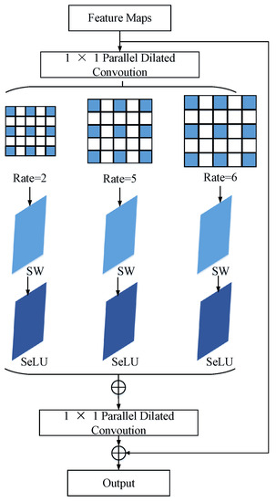
Figure 5.
Multi-feature representation. This module first performs parallel dilated convolution, then utilizes different multiple dilation rates (, , ) and passes corresponding SW operations, SeLU activation functions, and parallel dilated convolution. Residual connections are used to obtain the final feature map.
2.3. Alignment Attention Mechanism Based on Dynamic Feature Fusion
2.3.1. Dynamic Feature Fusion Alignment
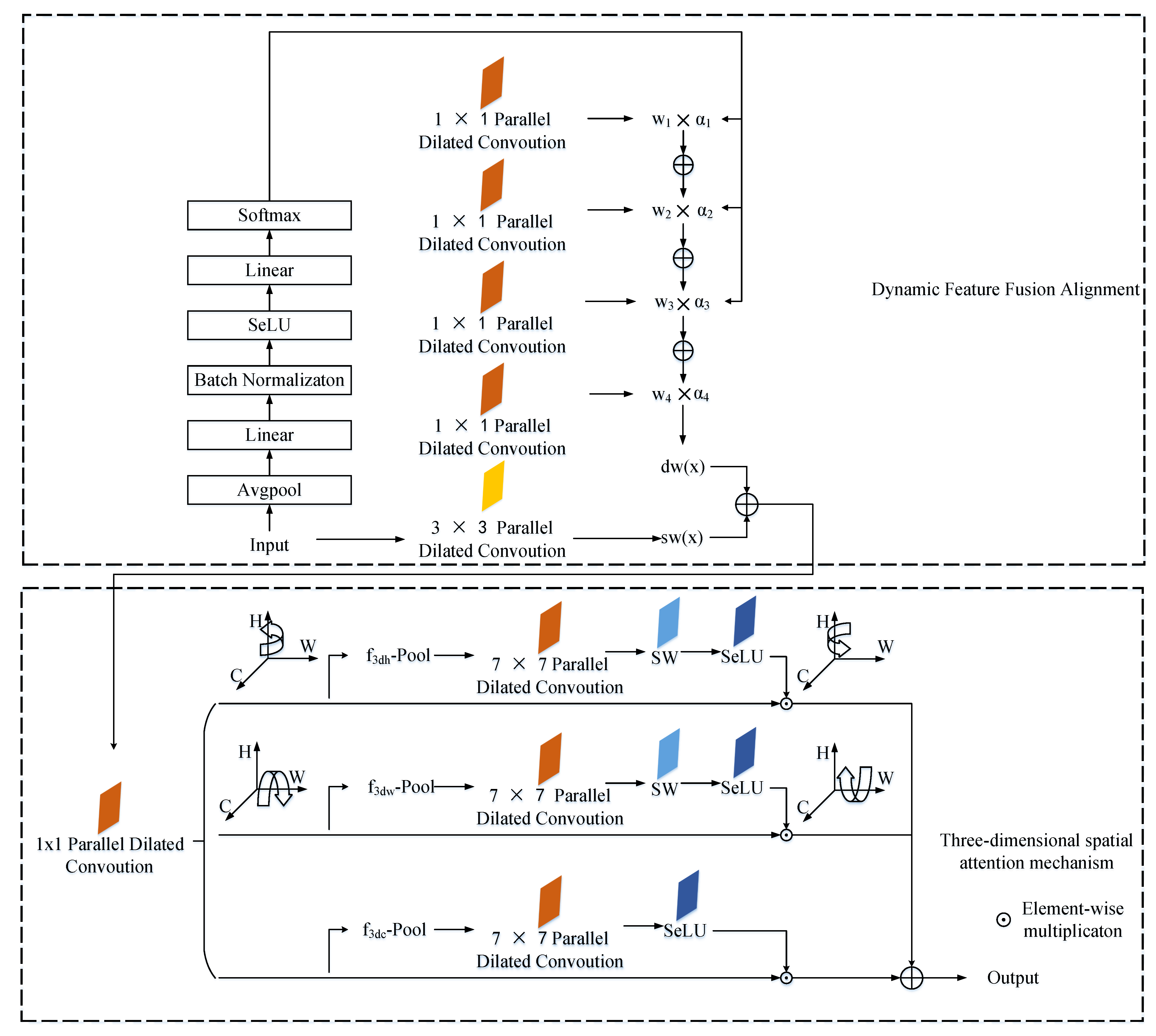
To effectively alleviate the difference between the source domain and the target domain and find the optimal balance point in the two domains, a dynamic feature-fusion-based alignment attention mechanism is proposed in this subsection, as shown in Figure 6. The specific expression is as follows:
where represents the overall weight, represents the dynamic alignment weight, and represents the static weight. The details are as follows:
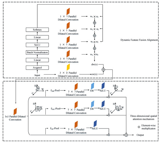
Figure 6.
Alignment attention mechanism based on dynamic feature fusion. The attention mechanism mainly consists of two parts: dynamic feature fusion alignment and 3D spatial attention mechanism. In the first section, there are operations, including Avgpool, Linear, BN, SeLU, Linear and Softmax. In the second section, operations are performed in three dimensions. The above operation can effectively reduce the difference between the source domain and the target domain.
- Dynamic alignment weight acquisition: Firstly, through average pooling, two linear layers, SeLU, and softmax operation, this operation is mainly to extract more effective features, suppress useless features, and, finally, obtain the dynamic scaling coefficient, . Then, four parallel dilated convolutions with branches are used to obtain four weights, and the final dynamic weights are obtained by the weights of the four branches and the dynamic scaling coefficients, which are specified as follows:where represents the softmax operation; and represent the second and first linear layer, respectively; S represents the SeLU activation function; and represents the average pooling operation. Then, we apply four parallel dilated convolutions to obtain the weights, , of the four branches.
- The static weights are obtained through a parallel dilated convolution.
Thus, the above can be expressed as follows:
2.3.2. Three-Dimensional Spatial Attention Mechanism
The three-dimensional spatial attention mechanism mainly includes three dimensions—height, width, and channel—and realizes the interaction of the above three dimensions. The above result is utilized to obtain through a parallel dilated convolution, and three replicas of it are made. On the first dimension of height, we rotate it 90 degrees along the H-axis to obtain feature . To obtain the attention weights on this dimension, we first retain rich features by pooling as follows:
where, f represents the input feature, ; represents average pooling; and represents max pooling.
Then, it goes through parallel dilated convolution layers, SW, and SeLU activation function operations in turn. Finally, it is rotated 90 degrees along the H-axis to restore the same shape as the original feature map. In the same way, the operation on the second dimension, width, is similar to the first one, except that it is rotated 90 degrees along the W-axis. In the third dimension, channel, it undergoes pooling, parallel dilated convolution layers, and SeLU activation functions. After obtaining the weights of the above three dimensions, the aggregation is performed in the following way:
where denotes switchable whitening, S denotes the SeLU activation function, denotes parallel dilated convolution, and denotes a rotation of 90 degrees.
2.4. Discrepancy Similarity Calculation
To address the marginal and conditional distributions efficiently, in this subsection, we propose Lie group maximum mean discrepancy (LGMMD) and Lie group conditional maximum discrepancy (LGCMMD).
2.4.1. LGMMD
Maximum mean discrepancy (MMD) is one of the typical methods to calculate the discrepancy, mainly by calculating the discrepancy of reproducing kernel Hilbert space (RKHS). The traditional MMD calculation is as follows:
where represents the RKHS established by feature mapping, and represents the feature mapping function, that is, by calculating the average of two samples over different distributions.
To calculate the marginal distribution between the source domain and the target domain, we optimize and improve it as follows:
where and denote the Lie group intrinsic means of the source and target domains, respectively. In a previous study [27,28], we found that the Lie group intrinsic mean can identify the potential characteristics of data samples, and the specific calculation method can be referred to in [27,28].
2.4.2. LGCMMD
Although LGMMD effectively reduces the distribution divergence, the conditional distribution divergence cannot be ignored. Therefore, in addition to the above, we also need to consider the conditional distribution divergence. Since the target domain does not contain labeled data samples, it is difficult to directly estimate the conditional distribution of the target domain. The usual solution is to adopt the predicted value of the target domain data as the pseudo label.
The posterior probabilities (i.e., and ) of the source and target domains are rather difficult to represent and are generally approximated by sufficient statistics of the class conditions, namely, and . Therefore, LGCMMD can be expressed as follows:
where C represents the number of kinds of data samples.
2.4.3. Dynamic Tradeoff Parameter
The probability of the two distributions can be obtained through the above calculation, and how to set the weights of the two distributions is a key problem to be solved in this research. In previous research, we found that average search and random guessing are commonly used methods [24]. Although the above two methods have been widely used in many models, they are relatively inefficient.
To address the above problems, we propose the dynamic tradeoff parameter in this subsection, which is as follows:
This parameter is updated in each iteration, and when the training converges, a relatively stable parameter value can be obtained.
2.5. Loss Function
The marginal distribution adaptation and conditional distribution adaptation loss functions are as follows:
respectively, where represents the domain feature extractor.
The class classifier is used to determine the category of the input data, and the corresponding loss function is expressed as follows:
where represents the cross-entropy loss, and represents the category classifier.
In summary, the overall objective function is expressed as follows:
where denotes the non-negative tradeoff parameter.
3. Experimental Results and Analysis
3.1. Experimental Datasets
In this part of the study, we chose three publicly available and challenging datasets and chose other state-of-the-art and competitive models to evaluate our proposed method, three of which are UC Merced [31] (UCM), AID [32], and NWPU-RESISC45 [33] (NWPU). The UCM dataset [31] contains 21 categories of scenes, and each category contains 100 images. The AID dataset [32] contains 30 categories of scenes, each of which has about 200 to 400 images. The NWPU dataset [33] contains 45 categories of scenes, and each category contains 700 images. These two types of datasets contain a large number of scene categories and are representative, including (1) high similarity between classes and diversity within classes; (2) the scene being rich. The above datasets come from different sensors, that is, HRRSI is obtained based on uncertain sensors. The main characteristics of the above two datasets can be referred to in the literature [1,2,3,4].
3.2. Experiment Setup
In the experimental setup, we performed six cross-domain scene classifications as follows: , where → represents the knowledge transfer from the source domain to the target domain. The other parameter settings are based on previous research [1,2,3,4,26], as detailed in Table 1, and the updating of parameters is mainly based on repeated experiments and iterations. To eliminate the contingency of the experiment, we conducted ten repeated experiments using randomly selected training and test data samples to obtain reliable experimental results.

Table 1.
Setting of experimental environment and other parameters.
3.3. Results and Comparison
The experimental results of our method and other methods are shown in Table 2. From Table 2, it can be observed that our proposed method has advantages over other methods and effectively improves the accuracy of cross-domain scene classification.
Table 2.
Experimental results of different methods (%).
From Table 2, it can be observed that our proposed approach has higher classification accuracy compared to other methods. When knowledge transfers from the source domain with a small data sample size to the target domain with a large data sample size, for example, in the experiment of UCM → AID, MRDAN improves 13.05% compared with ADA-DDA, and our method improves 0.12% and 13.17% compared with MRDAN and ADA-DDA, respectively. In the experiments of UCM → NWPU, the accuracy of ARMAN reaches 68.09%, the accuracy of MRDAN reaches 86.35%, and our method reaches 87.43%, which is 19.34% and 1.08% higher than them, respectively. When knowledge transfers from the source domain with a large amount of sample data to the target domain with a small amount of sample data, for example, in the NWPU → UCM experiment, the accuracy of ADA-DDA reaches 90.70%, the accuracy of DATSNET reaches 87.76%, and our method reaches 92.13%. Compared with the other methods, our proposed approach increased by 4.37% and 1.43% respectively. Furthermore, the average classification accuracy of our proposed method is improved compared with other methods.
There are several reasons for further analysis of the above experimental results:
- Our proposed approach extracts more and more useful features, which effectively expands the range of domain-invariant features. Drawing on the previous successful research basis [1,2,3,4], in addition to extracting the low-level, mid-level, and high-level features of the scene, this study also optimizes and improves the previous approach, increases the receptive field, reduces the dimension of the features, and extracts more effective features from different scales.
- From the experimental results, we found that when the number of data samples is small, the classification accuracy of the target domain will also decrease. For scene classification, data samples containing a large number of category information are crucial to the performance of the model, but obtaining a large number of data samples containing category information is tedious, expensive, and time-consuming work. Our proposed method reduces negative transfer to some extent.
- Our proposed alignment attention mechanism based on dynamic feature fusion effectively enhances the key features in the key region, suppresses the invalid features, and realizes the interaction of attention in the three-dimensional space. Based on previous research [1,2,3,4], this method was further optimized and improved to maximize the mining of key features in the scene.
4. Ablation Experiments
4.1. Influence of Different Modules on Cross-Domain Scene Classification
To demonstrate the effectiveness of different modules in our proposed approach, we constructed the following different ablation experiments: (1) a comparison of models without extracting low-level, middle-level, and high-level features against models with extracted low-level, middle-level, and high-level features; (2) a comparison of models that do not utilize multiple-feature spaces and models that utilize multiple-feature spaces; and (3) a comparison of models that do not utilize attention mechanisms with models that utilize attention mechanisms.
Since the number of categories and data samples in the UCM dataset is small, and the distribution difference between the UCM dataset and the AID dataset is also large, we still take UCM → AID as an example for ablation experimental analysis. From Table 3, we found that the accuracy of the model without extracting low-level, middle-level, and high-level features is relatively low, at only 85.73%, while the accuracy of the model without extracting low-level and middle-level features (that is, without using the Lie group machine learning method to extract low-level and middle-level features) is 86.97%, which is mainly because the model does not fully learn the domain-invariant features in the data samples. From Table 4, we found that the approach is optimized and improved based on previous research, and features at different scales are further extracted so that the model can effectively learn features at different scales and further expand the range of domain-invariant features. In addition, the model adopts parallel dilated convolution, which effectively reduces the feature dimension of the model and improves the adaptability of the model. From Table 5, we found that the model using the attention mechanism has more advantages in accuracy. Our proposed attention mechanism fully considers the weights on the three dimensions and adopts a dynamic way to adjust the parameters, avoiding the problem of local optima that may be caused by traditional methods.
Table 3.
Influence of low-level, middle-level, and high-level features.
Table 4.
Influence of multiple-feature spaces.
Table 5.
Influence of attention mechanisms.
4.2. KAPPA, Model Parameters, and Running Time Analysis
Table 6 shows the KAPPA coefficients, parameter sizes, and runtime of our proposed approach compared to other models. All models were tested under the same experimental conditions (hardware and software environment). From Table 6, we found that our proposed approach achieved better results in the three aspects mentioned above. Taking the UCM → AID experiment as an example, in terms of parameters, our approach effectively reduced the model’s parameters through the use of parallel dilated convolution and other operations, achieving reductions of 19.25 m and 9.98 m compared with the MRDAN [38] and AMRAN [35] models. In terms of the KAPPA coefficient, our method showed improvements of 0.2029 and 0.283 compared with the DATSNET [37] and CDAN+E [35] models. In terms of running time, reductions of 0.87 s and 0.893 s were achieved when compared with the BNM [35] and DAAN [36] models. Due to the fact that the model only requires classification without calculating backward gradients and, in addition, the model extensively utilizes operations such as Lie group intrinsic mean and parallel dilated convolution, the parameters are effectively reduced while also improving the model’s running time.
Table 6.
Comparison of KAPPA, model parameters, and running time.
5. Conclusions
In this study, we proposed a novel remote sensing cross-domain scene classification model based on Lie group spatial attention and adaptive multi-feature distribution. We tackled the problem of insufficient feature learning in traditional models by extracting features from low-level, middle-level, and high-level features. We further optimized the multi-scale feature space representation based on our previous research, effectively expanding the space of domain-invariant features. We also designed attention mechanisms for different dimensions of space, focusing on key regions through model training to suppress irrelevant features. The experimental results indicated that our proposed method has advantages in terms of model accuracy and the number of model parameters. Our proposed method is also able to automatically adjust the parameters of the marginal and conditional distributions, which greatly improves the effectiveness and robustness of the model.
In our study, we mainly considered the characteristics of the source domain and the target domain. Therefore, in future research, we will explore the use of other data (such as Gaode map data information) to further explore cross-domain scene classification. In the future, we will continue to explore the integration of Lie group machine learning and deep learning models to improve the robustness, interpretability, and comprehensibility of cross-domain scene classification models.
Author Contributions
Conceptualization, C.X., G.Z., and J.S.; methodology, C.X. and J.S.; software, J.S.; validation, C.X. and G.Z.; formal analysis, J.S.; investigation, C.X.; resources, C.X. and G.Z.; data curation, J.S.; writing—original draft preparation, C.X.; writing—review and editing, C.X.; visualization, J.S.; supervision, J.S.; project administration, J.S.; funding acquisition, C.X. All authors have read and agreed to the published version of the manuscript.
Funding
This work was partially supported by the National Natural Science Foundation of China (Research on Urban Land-use Scene Classification Based on Lie Group Spatial Learning and Heterogeneous Feature Modeling of Multi-source Data; grant no.: 42261068).
Institutional Review Board Statement
Not applicable.
Informed Consent Statement
Not applicable.
Data Availability Statement
The data associated with this research are available online. The UC Merced dataset is available for download at http://weegee.vision.ucmerced.edu/datasets/landuse.html (accessed on 12 November 2021). The AID dataset is available for download at https://captain-whu.github.io/AID/ (accessed on 15 December 2021). The NWPU dataset is available for download at http://www.escience.cn/people/Junwei_\Han/NWPURE-SISC45.html (accessed on 16 October 2020).
Acknowledgments
The authors would like to thank the four anonymous reviewers for carefully reviewing this study and giving valuable comments to improve this study.
Conflicts of Interest
The authors declare no conflict of interest.
Abbreviations
| AID | Aerial Image Dataset |
| BN | Batch Normalization |
| BW | Batch Whitening |
| CGAN | Conditional Generative Adversarial Network |
| CNN | Convolutional Neural Network |
| DCA | Discriminant Correlation Analysis |
| GAN | Generative Adversarial Network |
| GCH | Global Color Histogram |
| HRRSI | High-Resolution Remote Sensing Image |
| IW | Instance Whitening |
| LGCMMD | Lie Group Conditional Maximum Discrepancy |
| LGMMD | Lie Group Maximum Discrepancy |
| LN | Layer Normalization |
| MMD | Maximum Discrepancy |
| NWPU-RESISC | NorthWestern Polytechnical University Remote Sensing Image Scene |
| Classification | |
| OA | Overall Accuracy |
| ReLU | Rectified Linear Unit |
| RKHS | Reproducing Kernel Hilbert Space |
| SeLU | Scaled Exponential Linear Unit |
| SW | Switchable Whitening |
| UCM | University of California, Merced |
References
- Xu, C.; Shu, J.; Zhu, G. Adversarial Remote Sensing Scene Classification Based on Lie Group Feature Learning. Remote Sens. 2023, 15, 914. [Google Scholar] [CrossRef]
- Xu, C.; Zhu, G.; Shu, J. Scene Classification Based on Heterogeneous Features of Multi-Source Data. Remote Sens. 2023, 15, 325. [Google Scholar] [CrossRef]
- Xu, C.; Zhu, G.; Shu, J. A Combination of Lie Group Machine Learning and Deep Learning for Remote Sensing Scene Classification Using Multi-Layer Heterogeneous Feature Extraction and Fusion. Remote Sens. 2022, 14, 1445. [Google Scholar] [CrossRef]
- Xu, C.; Zhu, G.; Shu, J. A Lightweight and Robust Lie Group-Convolutional Neural Networks Joint Representation for Remote Sensing Scene Classification. IEEE Trans. Geosci. Remote Sens. 2022, 60, 1–15. [Google Scholar] [CrossRef]
- He, X.; Chen, Y.; Ghamisi, P. Heterogeneous transfer learning for hyperspectral image classification based on convolutional neural network. IEEE Trans. Geosci. Remote Sens. 2019, 58, 3246–3263. [Google Scholar] [CrossRef]
- Zheng, X.; Yuan, Y.; Lu, X. Hyperspectral image denoising by fusing the selected related bands. IEEE Trans. Geosci. Remote Sens. 2019, 57, 2596–2609. [Google Scholar] [CrossRef]
- Li, X.; Zhang, L.; Du, B.; Zhang, L. On gleaning knowledge from cross domains by sparse subspace correlation analysis for hyperspectral image classification. IEEE Trans. Geosci. Remote Sens. 2018, 57, 3204–3220. [Google Scholar] [CrossRef]
- Xiong, W.; Lv, Y.; Zhang, X.; Cui, Y. Learning to translate for cross-source remote sensing image retrieval. IEEE Trans. Geosci. Remote Sens. 2020, 58, 4860–4874. [Google Scholar] [CrossRef]
- Paris, C.; Bruzzone, L. A sensor-driven hierarchical method for domain adaptation in classification of remote sensing images. IEEE Trans. Geosci. Remote Sens. 2017, 56, 1308–1324. [Google Scholar] [CrossRef]
- Du, B.; Wang, S.; Xu, C.; Wang, N.; Zhang, L.; Tao, D. Multi-task learning for blind source separation. IEEE Trans. Image Process. 2018, 27, 4219–4231. [Google Scholar] [CrossRef]
- Zheng, X.; Yuan, Y.; Lu, X. A deep scene representation for aerial scene classification. IEEE Trans. Geosci. Remote Sens. 2019, 57, 4799–4809. [Google Scholar] [CrossRef]
- Yan, L.; Zhu, R.; Mo, N.; Liu, Y. Cross-domain distance metric learning framework with limited target samples for scene classification of aerial images. IEEE Trans. Geosci. Remote Sens. 2019, 57, 3840–3857. [Google Scholar] [CrossRef]
- Othman, E.; Bazi, Y.; Melgani, F.; Alhichri, H.; Alajlan, N.; Zuair, M. Domain adaptation network for cross-scene classification. IEEE Trans. Geosci. Remote Sens. 2017, 55, 4441–4456. [Google Scholar] [CrossRef]
- Liu, W.; Qin, R. A multikernel domain adaptation method for unsupervised transfer learning on cross-source and cross-region remote sensing data classification. IEEE Trans. Geosci. Remote Sens. 2020, 58, 4279–4289. [Google Scholar] [CrossRef]
- Yan, L.; Fan, B.; Liu, H.; Huo, C.; Xiang, S.; Pan, C. Triplet adversarial domain adaptation for pixel-level classification of VHR remote sensing images. IEEE Trans. Geosci. Remote Sens. 2019, 58, 3558–3573. [Google Scholar] [CrossRef]
- Bashmal, L.; Bazi, Y.; AlHichri, H.; AlRahhal, M.; Ammour, N.; Alajlan, N. Siamese-GAN: Learning invariant representations for aerial vehicle image categorization. Remote Sens. 2018, 10, 351. [Google Scholar] [CrossRef]
- Lu, X.; Gong, T.; Zheng, X. Multisource compensation network for remote sensing cross-domain scene classification. IEEE Trans. Geosci. Remote Sens. 2019, 58, 2504–2515. [Google Scholar] [CrossRef]
- Wang, J.; Chen, Y.; Hu, L.; Peng, X.; Philip, S.Y. Stratified transfer learning for cross-domain activity recognition. In Proceedings of the 2018 IEEE International Conference on Pervasive Computing and Communications (PerCom), Athens, Greece, 19–23 March 2018; pp. 1–10. [Google Scholar] [CrossRef]
- Pan, S.J.; Tsang, I.W.; Kwok, J.T.; Yang, Q. Domain adaptation via transfer component analysis. IEEE Trans. Neural Netw 2010, 22, 199–210. [Google Scholar] [CrossRef]
- Zellinger, W.; Grubinger, T.; Lughofer, E.; Natschläger, T.; Saminger-Platz, S. Central moment discrepancy (cmd) for domain-invariant representation learning. arXiv 2017, arXiv:1702.08811. [Google Scholar]
- Zhang, J.; Li, W.; Ogunbona, P. Joint geometrical and statistical alignment for visual domain adaptation. In Proceedings of the IEEE conference on computer vision and pattern recognition (CVPR), Honolulu, HI, USA, 21–26 July 2017; pp. 1859–1867. [Google Scholar] [CrossRef]
- Goodfellow, I.; Pouget-Abadie, J.; Mirza, M.; Xu, B.; Warde-Farley, D.; Ozair, S.; Courville, A.; Bengio, Y. Generative adversarial nets. IEEE Trans. Neural Netw. 2014, 27, 199–210. [Google Scholar]
- Shen, J.; Qu, Y.; Zhang, W.; Yu, Y. Wasserstein distance guided representation learning for domain adaptation. In Proceedings of the Thirty-Second AAAI Conference on Artificial Intelligence, New Orleans, LA, USA, 2–7 February 2018; p. 1. [Google Scholar] [CrossRef]
- Yu, C.; Wang, J.; Chen, Y.; Huang, M. Transfer learning with dynamic adversarial adaptation network. In Proceedings of the 2019 IEEE International Conference on Data Mining (ICDM), Beijing, China, 8–11 November 2019; pp. 778–786. [Google Scholar] [CrossRef]
- Tutsoy, O. Graph theory based large-scale machine learning with multi-dimensional constrained optimization approaches for exact epidemiological modelling of pandemic diseases. IEEE Trans. Pattern Anal. Mach. Intell. 2023, 45, 9836–9845. [Google Scholar] [CrossRef] [PubMed]
- LeCun, Y.; Bengio, Y.; Hinton, G. Deep learning. Nature. 2015, 521, 436–444. [Google Scholar] [CrossRef] [PubMed]
- Xu, C.; Zhu, G.; Shu, J. Robust Joint Representation of Intrinsic Mean and Kernel Function of Lie Group for Remote Sensing Scene Classification. IEEE Geosci. Remote Sens. Lett. 2020, 118, 796–800. [Google Scholar] [CrossRef]
- Xu, C.; Zhu, G.; Shu, J. A Lightweight Intrinsic Mean for Remote Sensing Classification With Lie Group Kernel Function. IEEE Geosci. Remote Sens. Lett. 2020, 18, 1741–1745. [Google Scholar] [CrossRef]
- Xu, C.; Zhu, G.; Shu, J. Lie Group spatial attention mechanism model for remote sensing scene classification. Int. J. Remote Sens. 2022, 43, 2461–2474. [Google Scholar] [CrossRef]
- Pan, X.; Zhan, X.; Shi, J.; Tang, X.; Luo, P. Switchable whitening for deep representation learning. In Proceedings of the IEEE/CVF International Conference on Computer Vision, Long Beach, CA, USA, 16–20 June 2019; pp. 1863–1871. [Google Scholar] [CrossRef]
- Yang, Y.; Newsam, S. Bag-of-visual-words and spatial extensions for land-use classification. In Proceedings of the 18th SIGSPATIAL International Conference on Advances in Geographic Information Systems, New York, NY, USA, 2–5 November 2010; pp. 270–279. [Google Scholar] [CrossRef]
- Xia, G.S.; Hu, J.; Hu, F.; Shi, B.; Bai, X.; Zhong, Y.; Lu, X. AID: A benchmark dataset for performance evaluation of aerial scene classification. IEEE Trans. Geosci. Remote Sens. 2017, 55, 3965–3981. [Google Scholar] [CrossRef]
- Cheng, G.; Han, J.; Lu, X. Remote sensing image scene classification: Benchmark and state of the art. Proc. IEEE 2017, 105, 1865–1883. [Google Scholar] [CrossRef]
- Yang, C.; Dong, Y.; Du, B.; Zhang, L. Attention-based dynamic alignment and dynamic distribution adaptation for remote sensing cross-domain scene classification. IEEE Trans. Geosci. Remote Sens. 2020, 60, 1–13. [Google Scholar] [CrossRef]
- Wang, J.; Chen, Y.; Feng, W.; Yu, H.; Huang, M.; Yang, Q. Transfer learning with dynamic distribution adaptation. ACM Trans. Intell. Syst.Technol. 2020, 11, 1–25. [Google Scholar] [CrossRef]
- Sun, B.; Saenko, K. Deep coral: Correlation alignment for deep domain adaptation. Proc. Eur. Conf. Comput. Vis. 2016, 105, 443–450. [Google Scholar] [CrossRef]
- Zheng, Z.; Zhong, Y.; Su, Y.; Ma, A. Domain adaptation via a task-specific classifier framework for remote sensing cross-scene classification. IEEE Trans. Geosci. Remote Sens. 2020, 60, 1–13. [Google Scholar] [CrossRef]
- Niu, B.; Pan, Z.; Wu, J.; Hu, Y.; Yuxin, H.; Lei, B. Multi-representation dynamic adaptation network for remote sensing scene classification. IEEE Trans. Geosci. Remote Sens. 2020, 60, 1–19. [Google Scholar] [CrossRef]
Disclaimer/Publisher’s Note: The statements, opinions and data contained in all publications are solely those of the individual author(s) and contributor(s) and not of MDPI and/or the editor(s). MDPI and/or the editor(s) disclaim responsibility for any injury to people or property resulting from any ideas, methods, instructions or products referred to in the content. |
© 2023 by the authors. Licensee MDPI, Basel, Switzerland. This article is an open access article distributed under the terms and conditions of the Creative Commons Attribution (CC BY) license (https://creativecommons.org/licenses/by/4.0/).