Article

Towards Optimal Variable Selection Methods for Soil Property Prediction Using a Regional Soil Vis-NIR Spectral Library

1
ZJU-Hangzhou Global Scientific and Technological Innovation Center, Hangzhou 311200, China
2
Institute of Agricultural Remote Sensing and Information Technology Application, College of Environmental and Resource Sciences, Zhejiang University, Hangzhou 310058, China
*
Author to whom correspondence should be addressed.
Remote Sens. 2023, 15(2), 465; https://doi.org/10.3390/rs15020465
Submission received: 23 November 2022 / Revised: 5 January 2023 / Accepted: 9 January 2023 / Published: 12 January 2023
(This article belongs to the Section Remote Sensing in Agriculture and Vegetation)

Abstract

:
Soil visible and near-infrared (Vis-NIR, 350–2500 nm) spectroscopy has been proven as an alternative to conventional laboratory analysis due to its advantages being rapid, cost-effective, non-destructive and environmentally friendly. Different variable selection methods have been used to deal with the high redundancy, heavy computation, and model complexity of using full spectra in spectral modelling. However, most previous studies used a linear algorithm in the variable selection, and the application of a non-linear algorithm remains poorly explored. To address the current knowledge gap, based on a regional soil Vis-NIR spectral library (1430 soil samples), we evaluated seven variable selection algorithms together with three predictive algorithms in predicting seven soil properties. Our results showed that Cubist overperformed partial least squares regression (PLSR) and random forests (RF) in most soil properties (R2 > 0.75 for soil organic matter, total nitrogen and pH) when using the full spectra. Most of variable selection can greatly reduce the number of spectral bands and therefore simplified predictive models without losing accuracy. The results also showed that there was no silver bullet for the optimal variable selection algorithm among different predictive algorithms: (1) competitive adaptive reweighted sampling (CARS) always performed best for the PLSR algorithm, followed by forward recursive feature selection (FRFS); (2) recursive feature elimination (RFE) and genetic algorithm (GA) generally had better accuracy than others for the Cubist algorithm; and (3) FRFS had the best model performance for the RF algorithm. In addition, the performance was generally better when the algorithm used in the variable selection matched the predictive algorithm. The outcome of this study provides a valuable reference for predicting soil information using spectroscopic techniques together with variable selection algorithms.

Graphical Abstract

1. Introduction

Being fundamental to life on Earth, soils are at the center of human security and sustainable development for the next generations [1,2]. The human population boom and rapid economic growth have led to an exponential demand for the use of soil to provide food, fiber, and livestock [3]. Under this tremendous pressure, soils are facing various degradations such as accelerated soil erosion, desertification, salinization, acidification, biodiversity loss, nutrient depletion, and loss of soil organic matter (SOM), challenging the fulfilment of UN Sustainable Development Goals (SDGs) [2,4]. To make soils more sustainable, the demand for up-to-date soil information is soaring to inform practical land management [5,6]. Being labor-intensive, time-demanding, costly and involved with environmental pollutants, conventional laboratory analysis cannot meet the need for soil monitoring [7,8]. Under this context, soil spectroscopy has emerged as a rapid, cost-effective, environmentally friendly and non-destructive technique for measuring soil information [8,9].
Previous studies have shown that visible and near-infrared (Vis-NIR, 350–2500 nm) spectroscopy can be used to accurately predict soil properties such as SOM, total nitrogen (TN), pH and cation exchange capacity (CEC) and particle size fractions (i.e., clay, silt, sand) [10,11,12,13,14,15,16,17,18]. The overtones and combinations of fundamental vibrations are the fundamentals of Vis-NIR spectra for soil property prediction [7]. Despite the broad and overlapping bands, Vis-NIR contains valuable information on soil organic and inorganic components: (1) the absorptions between 400–780 nm are associated to minerals with iron oxide; (2) SOM has a broad absorption in the visible region dominated by chromophores and soil color; (3) clay minerals have absorptions in the vis–NIR region resulting from metal-OH bend and O–H stretch combinations, and therefore minerals determined soil properties such as clay and CEC have spectral response [7]; and (4) TN and pH do not have a direct spectral response in the vis-NIR region while they can be accurately predicted when they have high correlation with SOM and clay minerals [7].
Due to the high redundancy, heavy computation, and model complexity of full spectra, various variable selection methods have been adopted to address these limitations. The adoption of variable selection for regression models is also in favor of the principle of parsimony, that is, a simpler model with fewer parameters is favored over more complex models with more parameters when the model performance is similar. Cécillon et al. (2008) successfully applied variable importance in projection (VIP) to increase the prediction performance of Partial Least Squares Regression (PLSR) in predicting soil biological properties [19]. Vohland et al. (2014) first introduced the use of competitive adaptive reweighted sampling (CARS) in soil spectroscopy, and they found that CARS-PLSR was markedly more accurate than the full spectrum-PLSR model in predicting soil organic carbon (SOC), TN, C/N, and pH [20]. Hong et al. (2018) compared the performance of CARS and genetic algorithm (GA) in SOM modelling, and they concluded that GA yielded better accuracy than CARS [21]. Guo et al. (2021) found that CARS was superior to the successive projections algorithm (SPA) in selecting effective variables for the spectroscopic prediction of SOM, available phosphorous (AP) and available potassium (AK) using PLSR and SVM models [22]. Bai et al. (2022) recently found that CARS performed better in SOC than Ant colony optimization (ACO) using Vis-NIR spectroscopy [23]. However, most of the algorithms in these variable selection methods are mainly dealing with linear relationships (e.g., PLSR), and the use of non-linear algorithms based variable selection methods such as Boruta and Recursive Feature Elimination (RFE) remains poorly explored in soil prediction using Vis-NIR spectroscopy [24,25,26,27,28].
To address the aforementioned knowledge gap, the objectives of this study are two-fold: (1) comparison of the ability of soil property prediction using three predictive algorithms and regional soil spectral library; and (2) evaluation of the potential of variable selection algorithms with linear and non-linear algorithms in improving the performance. The outcome of this study can provide a reference for determining the optimal variable selection for improving model parsimony and accuracy in the spectroscopic modelling of soil information.

2. Materials and Methods

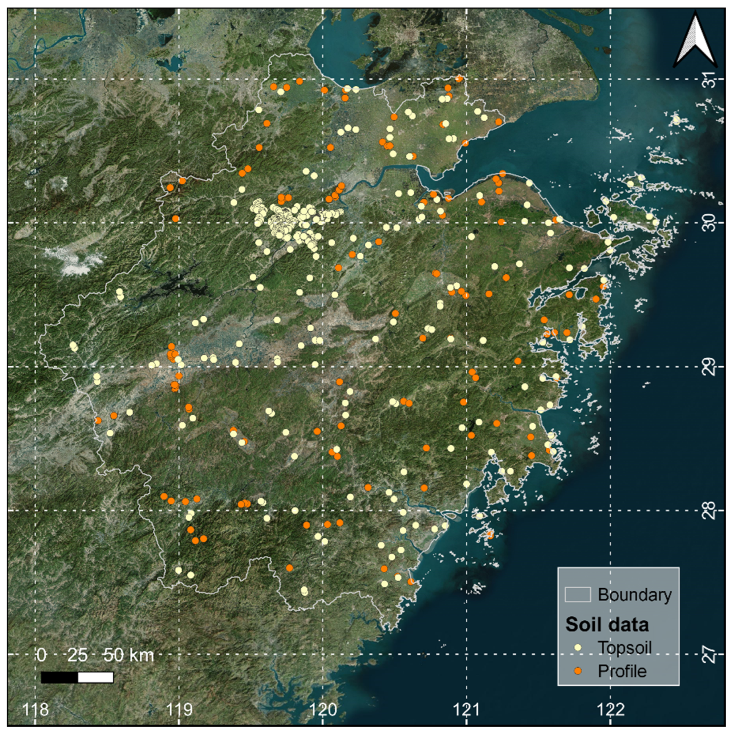
2.1. The Zhejiang Soil Spectral Library

Zhejiang Province is in the southeast coastal region of China (Figure 1). It has a total area of 105,000 km2, and its elevation ranges from 0 to 1907 m with an ascending gradient from the southwest part to the northeast part [29]. Zhejiang has a subtropical monsoon climate with a mean annual temperature of 15–18 °C and a mean annual precipitation of around 2000 mm. It has been cultivated under rice for more than a thousand years. The dominant soil types in the region are Anthrosols, Cambisols, Fluvisols, Leptisols, Luvisols and Acrisols in the World Reference Base (WRB) soil classification system [30,31].
The first version of the Zhejiang Soil Spectral Library (ZSSL) is composed of soil data collected from different projects with a time span from 2011 to 2021 [32,33,34,35,36]. The ZSSL includes 1430 soil samples collected mainly from the cropland and forest, covering the entire Zhejiang Province (Figure 1). Due to the different soil sampling designs for various purposes, 588 soil samples were collected in soil profiles (sampling sites were determined by soil surveyors on the knowledge of soil types), and the remaining 842 soil samples were collected only at the topsoil (0–20 cm) by a soil auger or probe. All the soil samples were air-dried, ground and sieved to less than 2 mm before the laboratory analysis and spectral measurement. Soil organic matter (SOM) was determined by the H2SO4–K2Cr2O7 oxidation method at 180 °C for 5 min [37]. TN was measured by the semi-micro Kjeldahl method. Soil pH was measured at 1:1 soil:water suspension. CEC was measured by NH4OAc (pH = 7.0) exchange method [37]. Soil particle size factions (i.e., clay, silt and sand) were determined by the pipette method [37]. The number of soil samples with SOM, TN, pH, CEC, and particle size fractions records were 1429, 1264, 1429, 689 and 589.
The spectral measurement was performed on the soil samples placed in a Petri dish 10 cm in diameter and 1.5 cm deep (about 100 g soil). Soil Vis-NIR spectra were measured using FieldSpec 3 Spectrometer before 2018 and FieldSpec 4 Spectrometer since 2018 (Analytical Spectral Devices Inc., Boulder, CO, USA). Both spectrometers have similar instrumental parameters with a spectral range of 350–2500 nm and a spectral sampling resolution of 1 nm. They were equipped with a high-intensity contact probe for soil spectral measurement and a Spectralon panel with 99% reflectance for white reference (Analytical Spectral Devices Inc., Boulder, CO, USA). To minimize noise and maximize the signal-to-noise ratio, three random measurements with ten internal scans were recorded for each soil sample. The resulted 30 spectra were then averaged into one representative spectrum per each soil sample.

2.2. Spectral Pre-Processing

Soil Vis-NIR spectra were reduced to 400–2450 nm to eliminate the signal noise at the spectral edges. In addition, to further reduce noise and amplify the signals, the spectra were processed using the Savitzky–Golay smoothing with a window size of 21 and polynomial order of 2 together with first derivatives, followed by standard normal variate transformation, which performed best in our preliminary test [38]. The spectra were trimmed to 5 nm resolution (remaining 410 spectral bands) to speed the computation efficiency while not losing model accuracy [39,40].
After spectral pre-processing, the sequence of different methods was listed below: (1) using seven variable selection methods to identify the most relevant variables; (2) optimizing three predictive algorithms based on the most relevant variables; and (3) validating the model performance. Since variable selection algorithms also included predictive algorithms to identify the most relevant variables; therefore, we started to introduce predictive algorithms in Section 2.3, then variable selection algorithms in Section 2.4 and ended with model evaluation in Section 2.5.

2.3. Predictive Algorithms

In this study, three commonly used predictive algorithms, namely PLSR, Cubist and Random Forests (RF) were investigated.
PLSR is a widely used algorithm for soil spectral modelling. It can effectively reduce the dimension of spectral data and retain the highly correlated latent variables (LVs) by projecting the predictor variables and the response variable to a new space [41]. The number of LVs in PLSR was optimized from 2 to 30 with an interval of 2 by 10-fold cross-validation.
Originating from M5 algorithm, Cubist is a piecewise linear decision tree algorithm [42]. It recursively splits the response variables into several subsets within which the subset has similar predictor variables. These splits are defined by a list of hierarchically ordered rules that have the following format: IF [condition], THEN [linear regression model]; ELSE [go to the next rule]. When a sample satisfies the condition of a specific rule, a corresponding linear regression model is then used to predict the response variable.
Developed from the Classification and Regression Tree, RF consists of multiple trees generated by a combination of bagging and random selection of predictor variables applied at each split of the trees [43]. For regression purposes, the final prediction result of RF is the weighted mean of the prediction from all trees. The RF prediction would be quite stable when the tree number is large enough, and therefore 500 trees were used in this study. The number of variables randomly sampled as candidates at each split (mtry) in RF was optimized from 2 to 20 with an interval of 2 by 10-fold cross-validation.
The PLSR, Cubist and RF were implemented in R packages “pls”, “Cubist”, “randomForest” and “caret”.

2.4. Variable Selection Algorithms

Seven variable selection algorithms, including CARS, VIP, ACO, GA, Boruta, RFE, and Forward Recursive feature selection (FRFS) were compared.
Proposed by Li et al. (2009) [44], the CARS adopts an exponentially decreasing function to eliminate the predictors with small coefficients, and then fits a PLSR model using the remaining predictors and calculates model performance (RMSE) by k-fold cross-validation. The predictors in the model with the lowest RMSE are determined as the finally selected predictors. It should be noted that PLSR is the only available algorithm for CARS (Table 1).
VIP is an indicator to determine the importance of each variable in the PLSR model [40]. The VIP is calculated by the equation below:
VIP k ( a ) = K a w a k 2 ( SSY a SSY t )
where VIP k ( a ) is the importance of the kth predictor in a PLSR model with a LVs, wak is the loading weight of the kth predictor in the ath LV, SSY a and SSY t are the explained and total sum of squares of response variable by a PLSR model with a LVs, and K is the total number of predictors. A greater VIP indicates a high variable importance, and a threshold of 0.5 was used in this study. Since VIP is derived from the PLSR model, PLSR is the only available algorithm for VIP (Table 1).
The ACO was developed by Dorigo (1992) [45], it mimics the foraging behavior of ants in a colony, and a pheromone is used for simulating the local interactions and communications among ants. The ants behind determine the direction of foraging based on the pheromones left in the path. When a path is shorter, ants walking on that path will leave more pheromones behind, which will attract more ants to choose that path. If the number of ants walking through the path is higher, the number of pheromones left behind is also higher, which leads to a positive feedback mechanism. For the application of variable selection, ACO tries to minimize the loss function of the predictive model, simulates the foraging behavior of ants, and seeks the important variable based on the change of pheromones on the path. As indicated in Table 1, different algorithms can be used for ACO. The ACO algorithm was performed in R package “FSinR”.
GA mimics Darwinian forces of natural selection to find the optimal variable for the target model [46]. It first generates an initial set of candidate solutions and calculates their fitness score by a pre-defined fitness function. This set of candidate solutions is regarded as a population, and each candidate solution as an individual. The individuals with the best model performance (RMSE) are combined randomly to produce offspring of the next population. During this step, individuals are selected and undergo crossover (mimicking genetic reproduction) and are subject to random mutations with a low random probability. This procedure is repeated at given times (it can be defined by users) to create many generations that can have better model performance. The GA terminates if the population has converged; in other words, it does not produce offspring that are significantly different from the previous generation. For the application of variable selection, the individuals are subsets of predictors which are marked either included or excluded. As indicated in Table 1, GA is applicable to different algorithms. The GA algorithm was performed in R package “caret”.
Boruta first duplicates the data set and then shuffles its predictors in each column (which are called shadow predictors) [47]. Secondly, it trains a RF algorithm and fits the model using the original and shuffled data sets combined, and then evaluates the variable importance (Z score) for each predictor. In each iteration, it checks whether a real predictor has higher importance than the best of its shadow predictors and marks the predictor as either confirmed (important) or rejected (unimportant). At last, it stops when all the predictors are confirmed or rejected. It should be noted that RF is the only available algorithm for Boruta (Table 1). The Boruta algorithm was performed in R package “Boruta”.
RFE works as follows: (1) fit a model using all the n predictors, calculate model performance (RMSE) by k-fold cross-validation as well as the variable importance (determined by variable permutation); (2) remove the least important predictor from the pool, refit the model, assess model performance and remove the least important predictor again; (3) repeat the second procedure down to a pool from n to 1 with a step of 1; and (4) determine the optimal number of predictors by taking the model with the best performance (RMSE). The RFE was implemented in R package “caret” with different options for the algorithm including PLSR, Cubist and RF (Table 1).
FRFS was initially proposed by Xiao et al. (2022) [48] to select the most relevant variables in pedotransfer functions, and it is for the first time to be tested in spectral modelling. FRFS adopts a forward selection strategy that includes steps: (1) fit a model using all the n predictors, and calculate the variable importance (determined by variable permutation); (2) select the most important predictor (only one) to fit an initial model, and calculate the model performance (RMSE) by k-fold cross-validation (note that there is only one predictor in the pool); (3) fit a list of models using 2 predictors (the combinations of predictor(s) in the pool and one of the remaining predictors), calculate their model performance, and recorded the model with the best performance; (4) update the pool by taking the predictors from the best model in the last step; and (5) repeat steps 3 and 4 by increasing the number of predictors from 3 to n. The predictors in the model with the best performance are selected for the final model. It is possible to set an early stop when the model performance starts to decrease for a large number of predictors (>50). The FRFS algorithm was performed in R and the current version supports PLSR, Cubist or RF as the algorithm (Table 1). The R code is available at https://zenodo.org/deposit/7340208 (accessed on 22 November 2022).

2.5. Model Evaluation

In this study, 10-fold cross-validation was used for robust model evaluation [49]. The 10-fold cross-validation includes several steps: (1) the whole data is randomly split into 10 equal-sized subsets; (2) each subset is taken out for validation set, and the remaining 9 subsets are used to fit the model that is used to predict the validation set; and (3) when all the subsets have been predicted, their predictions are combined (same size of whole data) to be evaluated against the observed data. Two performance indicators, including coefficient of determination (R2) and RMSE, were used to evaluate the model performance. A good model should have high R2 and low RMSE.
R 2 = 1 i n ( y ^ i y i ) 2 i n ( y i y ¯ ) 2
RMSE = i n ( y i ^ y i ) 2 n
where y i and y ^ i are observation and prediction for sample i, y ¯ is the mean of all the observations, and n is the number of samples.

3. Results

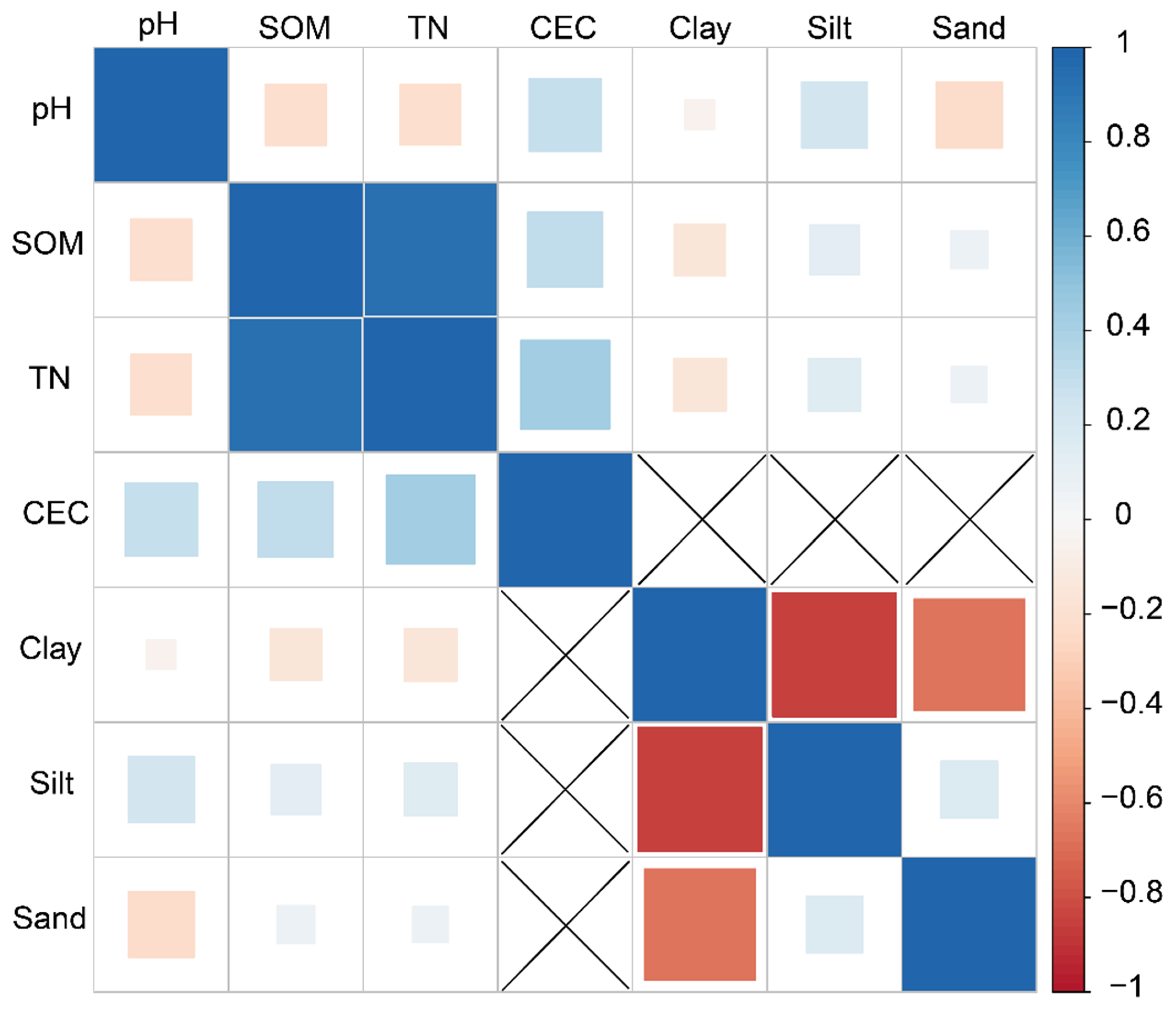
3.1. Statistics of Soil Properties and Their Correlations

Table 2 presents the statistics of seven soil properties recorded in ZSSL. SOM ranged from 0.80 to 141.70 g kg−1, showing a heterogeneity with a coefficient of variation (CV) of 62%. The distribution of SOM was highly right-skewed (skewness of 1.40) and highly fat-tailed (kurtosis of 9.33). TN had a similar distribution to SOM, with a range from 0.01 to 1.28 g kg−1, CV of 61%, skewness of 0.83 and kurtosis of 4.82. Ranging from 3.30 to 9.69, pH had a low heterogeneity (CV of 22%) and positive skewness (0.83), and it showed a normal distribution (kurtosis around 3). With a positive skewness (0.84) and laplace distribution (kurtosis of 5.67), CEC had a moderate CV (0.39%) with minimum and maximum at 1.20 and 37.00 cmol kg−1. Except for clay, sill and sand were nearly in a normal distribution (kurtosis near 3). Silt showed a negative skewness (−0.47), while clay and sand were positively skewed.
The correlation among seven soil properties is shown in Figure 2. SOM and TN were highly positively correlated with a correlation coefficient (r) at 0.9. Both SOM and TN were positively correlated to CEC with r of 0.31 and 0.43, while they were slightly negatively correlated to pH (r around −0.21). Soil pH showed a low negative correlation to sand (r = −0.24) and positive correlation to silt (0.24). Among particle size fractions, clay was positively correlated to silt (r = −0.84) and sand (r = −0.68), while the correlation between silt and sand was relatively low (r = −0.18).

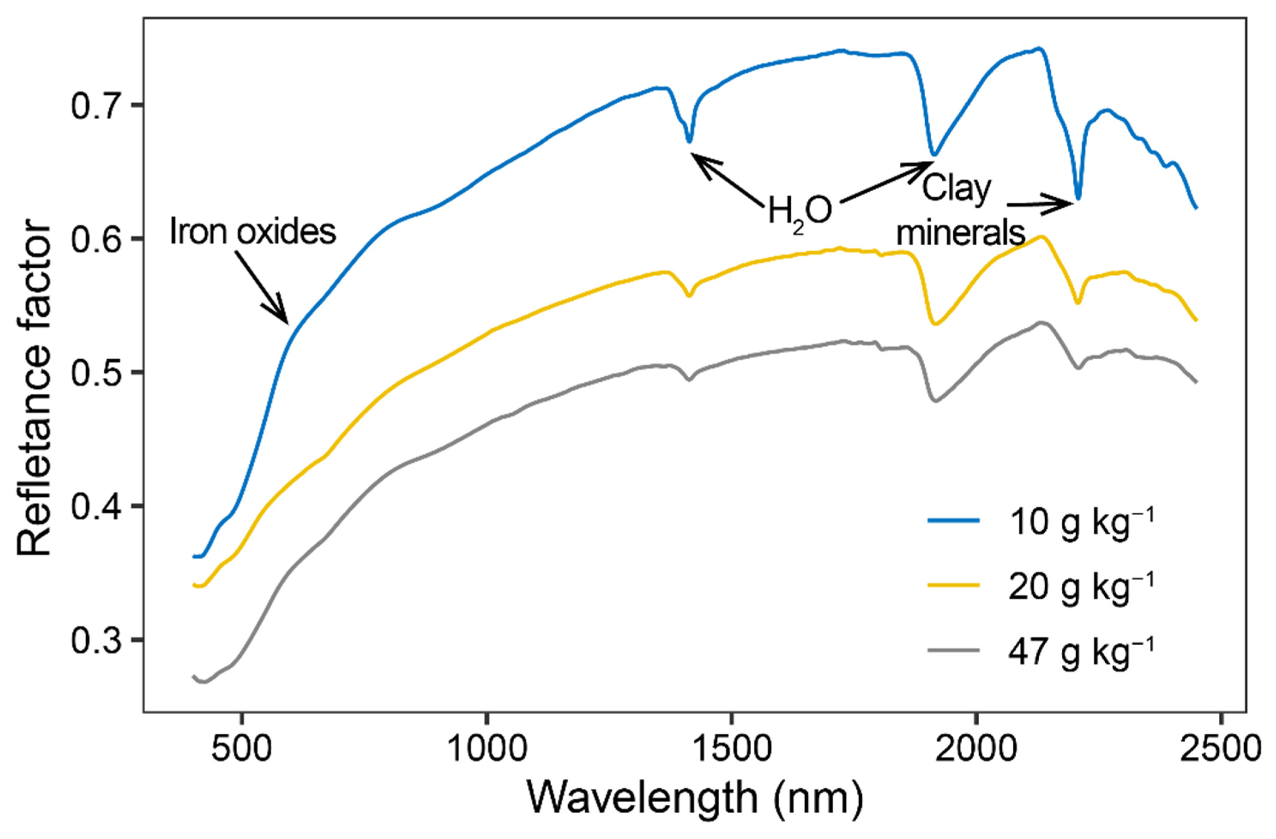
3.2. Soil Spectral Characteristics of Several Representative Soil Samples

Figure 3 shows the reflectance spectra of soil samples with different SOM levels in the ZSSL. Generally, the reflectance of soil spectra decreased with the increasing SOM content: the soil with low SOM had much higher reflectance and vice versa. In the spectral region from 550 to 800 nm, electronic transitions are dominated mainly by iron oxides and SOM (Figure 3). Clear water absorption bands were found around 1400 and 1900 nm, and the clay minerals had strong absorption between 2200 and 2300 nm (Figure 3).

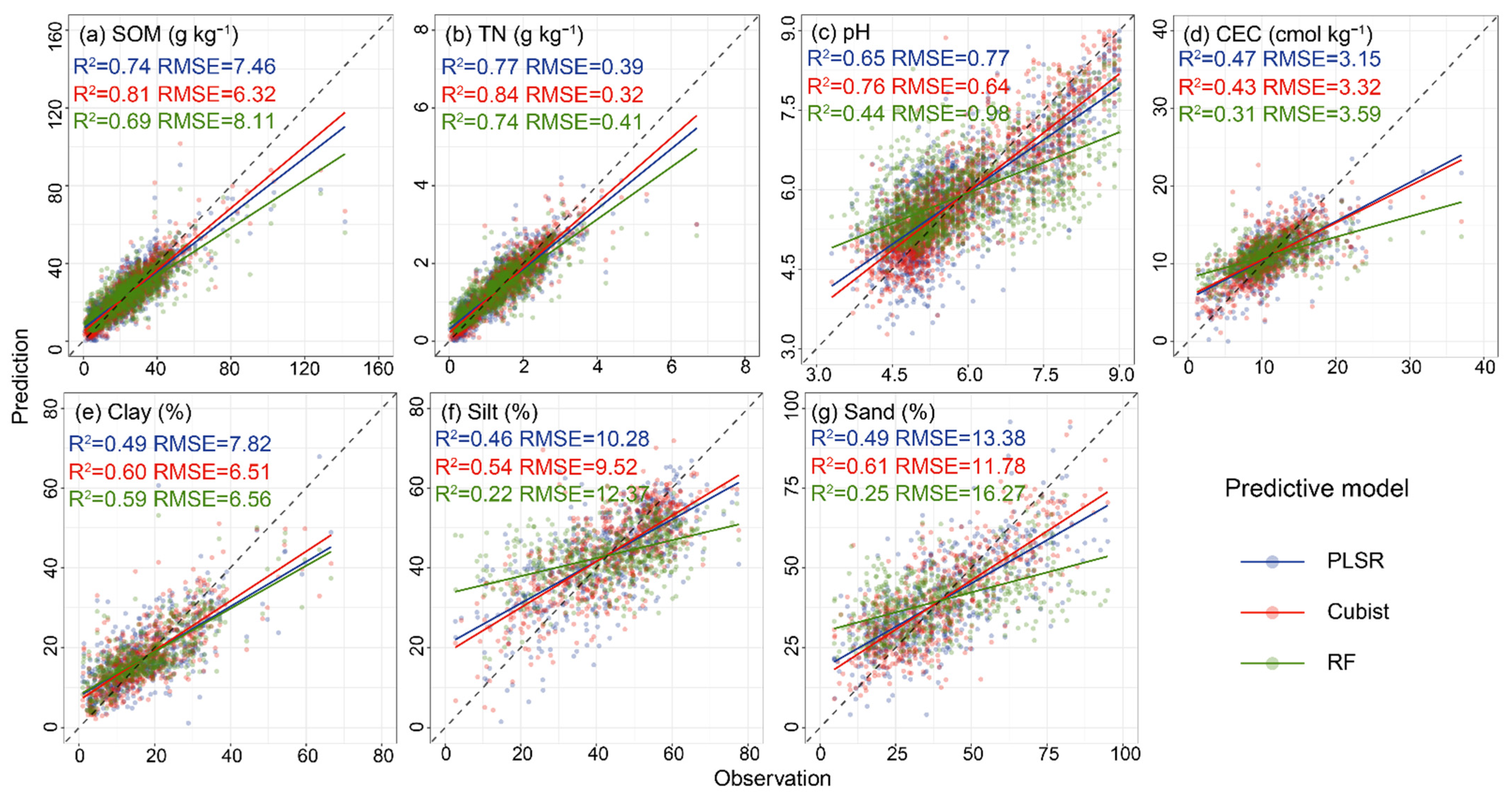
3.3. Performance of Three Predictive Algorithms Using Full Spectra

Figure 4 presents the performance of three predictive algorithms (PLSR, Cubist and RF) in predicting soil properties using full spectra (410 spectral bands). The 10-fold cross-validation results showed that full vis-NIR spectra could well predict SOM (R2 of 0.69–0.81), TN (R2 of 0.74–0.84) and pH (R2 of 0.44–0.76). Moderate performance was found for clay (R2 of 0.49–0.60), silt (R2 of 0.22–0.54) and sand (R2 of 0.25–0.61), while low performance was found for CEC (R2 of 0.31–0.47). The results also indicated that Cubist had the best model performance for most soil properties (SOM, TN, pH, clay, silt and sand), except for CEC, of which PLSR had slightly better accuracy.

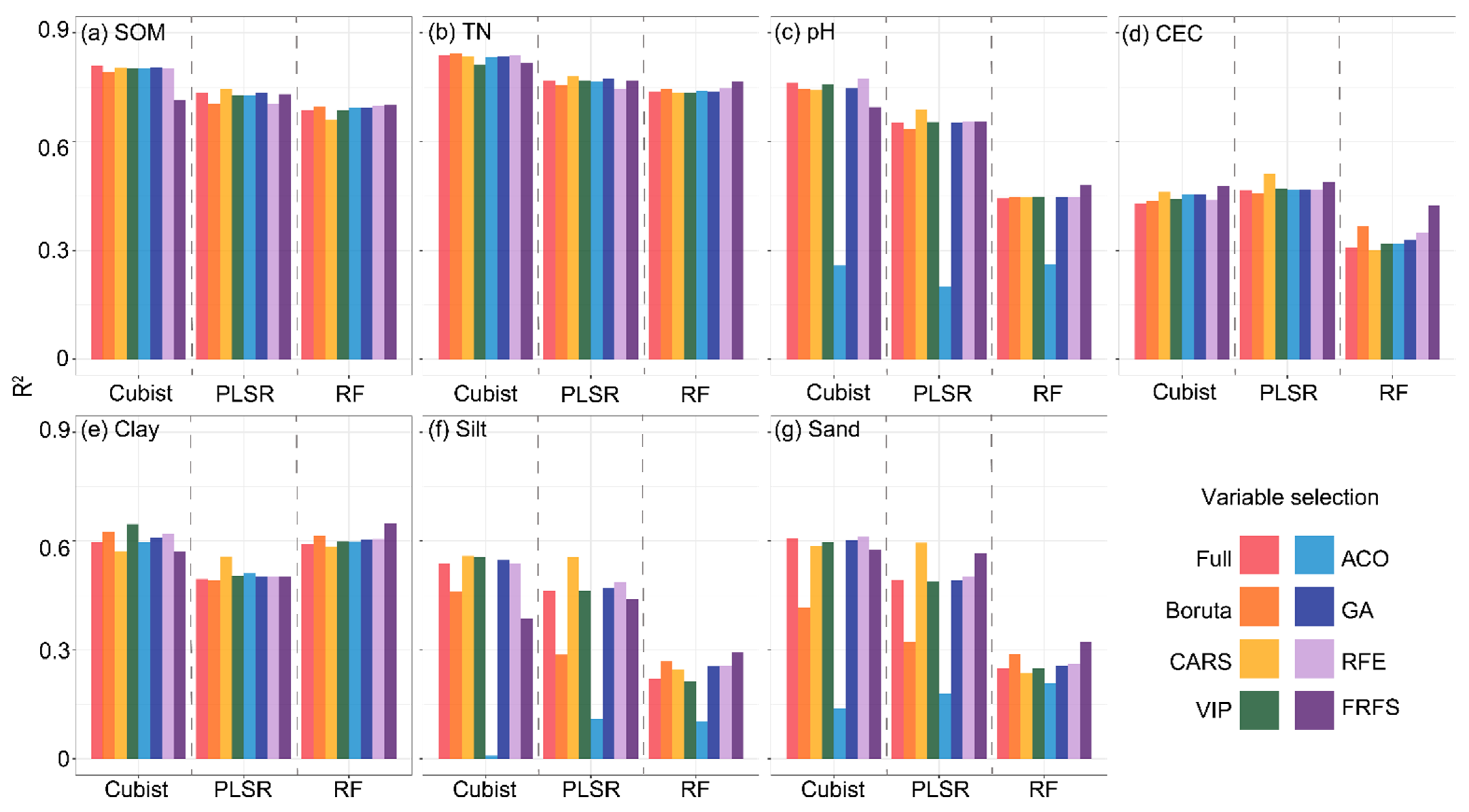
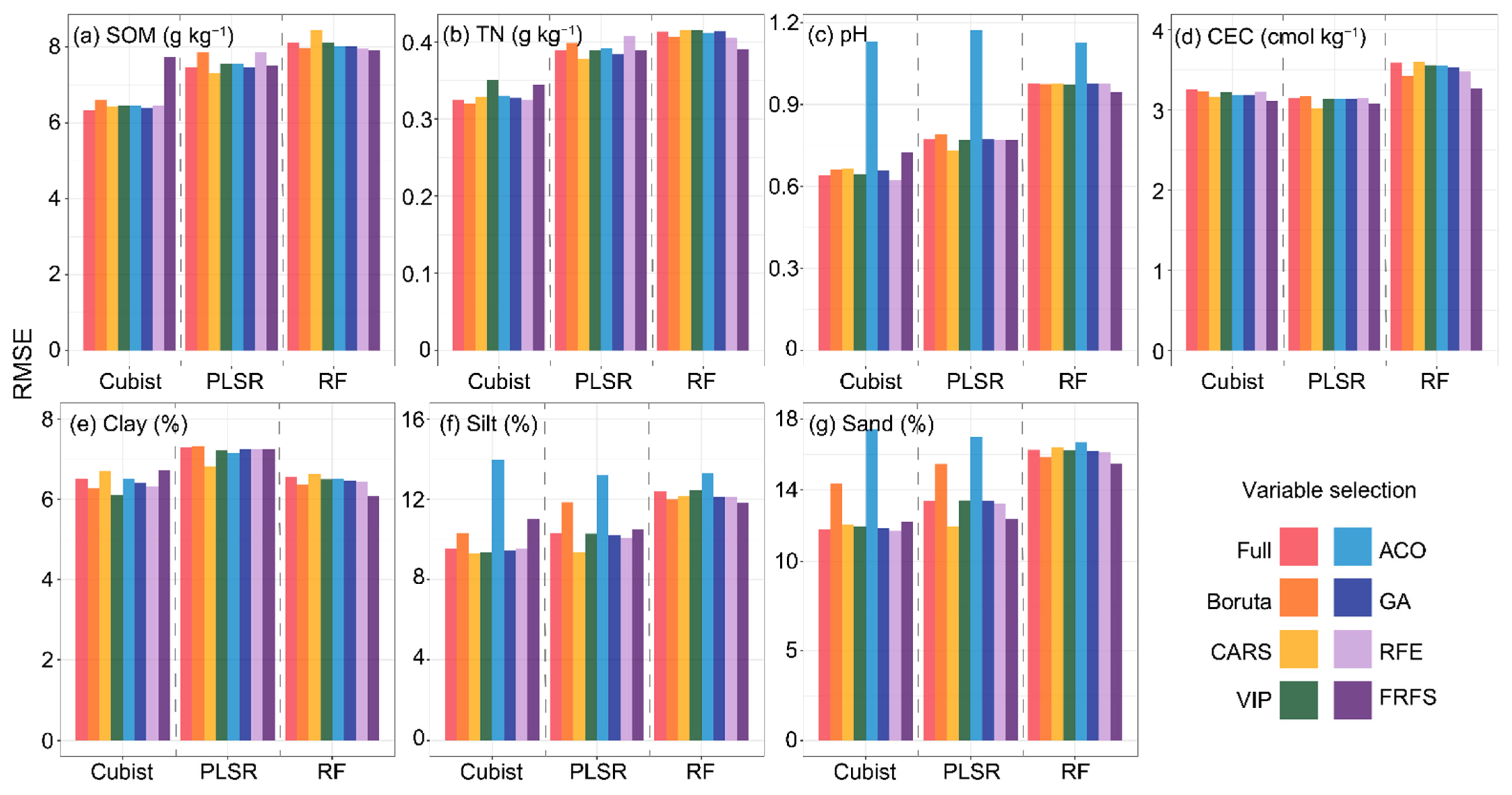
3.4. Performance of Three Models after Spectral Variable Selection

After variable selection, the number of spectral bands was effectively reduced for all the variable selection algorithms (Figure 5 and Figures S1–S6). Here, we took SOM for an example as shown in Figure 5. The kept spectral bands differed a lot among variable selection algorithms as well as the different algorithms. FRFS selected the lowest number of spectral bands, ranging from 11 for RF to 55 for PLSR. CARS only kept 44 spectral bands widely distributed in the vis-NIR region. Boruta and VIP selected 200 and 334 spectral bands, respectively. Both ACO and GA eliminated 25% to 50% spectral bands for three algorithms.
Figure 6 and Figure 7 present the model performance (R2 and RMSE) of three predictive algorithms together with seven variable selection methods. The results showed that the predictive algorithms built on selected spectral bands generally had similar or even better model performance to the predictive algorithms using full spectra. The best variable selection algorithm varied with different predictive algorithms: (1) for PLSR algorithm, CARS always performed best, followed by FRFS; (2) for Cubist algorithm, RFE and GA generally had better accuracy than others; and (3) for RF algorithm, FRFS was the best variable selection algorithm among different soil properties. It should also be noted that when the algorithm in variable selection matched with the predictive algorithm (e.g., CARS with PLSR, Boruta with RF), the model performance was better than the same predictive algorithm together with other algorithms.

4. Discussion

4.1. The Ability of Soil Vis-NIR Spectroscopy to Predict Soil Properties

The 10-fold cross-validation results showed that the best predictive model using full spectra could well predict SOM, TN and pH with R2 over 0.75 (Figure 4), which was in line with previous studies [50,51,52,53]. SOM is the most frequently predicted soil property by Vis-NIR spectroscopy, its overtones and combination bands in the Vis-NIR region result from the stretching and bending of N-H, C-H, and C-O groups [7]. Being highly correlated to SOM, and having a direct spectral response, TN is also among the primary soil properties that can be well predicted by Vis-NIR spectra [54]. Despite the fact that soil pH is not expected to have a direct spectral response in the Vis-NIR region, it can still be well predicted mainly due to its correlation to SOM, TN and clay [55], which is confirmed in our study (Figure 2).
Moderate model performance was found for soil particle size fractions (i.e., clay, silt and sand) with R2 of 0.54–0.61. The success of soil particle size fractions prediction results from their high correlation to clay minerals (e.g., goethite, hematite, kaolin, smectite), which have direct spectral responses around 480, 660, 880, 930, 1400, and 2200–2400 nm [7,56].
The predictive ability of Vis-NIR spectroscopy in CEC was somewhat limited (R2 of 0.47), which is in contrast with most previous studies finding that CEC can be well predicted by Vis-NIR spectra [7,15,57,58,59]. Similar to the previous study from Viscarra Rossel et al. [60], the low accuracy of CEC prediction may result from its weak correlation to clay minerals.
Regarding three predictive algorithms, Cubist generally overperformed PLSR and RF for most soil properties. Our results are in agreement with previous studies that Cubist had a better model performance than PLSR and RF in predicting soil properties (e.g., SOC, TN, sand, clay, soil salinity) at a regional scale either using limited samples (<100 samples) or a large soil spectral library [60,61,62]. It seems that RF always goes into an over-fitting situation (much better calibration accuracy than validation accuracy) even the parameters are well-tuned using cross-validation. It implies that RF is not good at dealing with multicollinearity problems, at least in soil spectroscopic modelling.

4.2. The Potential of Variable Selection in Spectroscopic Prediction of Soil Properties

In this study, we systematically evaluated seven variable selection algorithms which used both linear and non-linear algorithm. The results showed that most of the variable selection algorithms can reduce the spectral bands while keep similar or even improve model performance to those models using full spectra (Figure 5, Figure 6 and Figure 7), which is in line with previous studies [19,20,21,22,23,63,64,65]. However, there was no silver bullet for the optimal variable selection algorithm among different predictive algorithms: (1) CARS always performed best for the PLSR algorithm, followed by FRFS; (2) RFE and GA generally had better accuracy than others for the Cubist model; and (3) FRFS had the best model performance for the RF algorithm. Therefore, it is necessary to tune the optimal variable selection algorithm when using several different predictive algorithms for the spectroscopic prediction of soil information.
Additionally, we found that the model performance was generally better when the algorithm applied in variable selection matched the predictive algorithms. It is an important issue that remains poorly explored in previous studies [22,66,67]. The rationale is that the algorithm used in the variable selection algorithm determines how to calculate variable importance, which can be invalid when the predictive model does not match. For example, the CARS uses PLSR as the algorithm so that the rule to determine variable importance obeys the linear relationship. When we use non-linear RF as the predictive model, the CARS selected variable can be useless in dealing with the non-linear correlations. Therefore, we suggest matching the algorithm of the variable selection algorithm with the predictive algorithm to keep a good model performance in soil spectroscopic prediction.

4.3. Limitations and Perspectives

Firstly, we only consider the interaction between the variable selection algorithm and predictive algorithms using global modelling strategies. Therefore, some local modelling strategies such as LOCAL, locally weighted regression (LWR), RS-LOCAL, and memory-based learning (MBL) should be investigated in future studies when using large soil spectral libraries [68,69,70,71,72]. This is quite important because the local calibration set will dramatically change thus requiring a more flexible and robust variable selection algorithm.
Secondly, since an effective variable selection algorithm designed for deep learning models (such as multilayer perceptron, and convolutional neural networks) has not been well developed, we did not test these deep learning models in our study. Therefore, more investigations are required to determine the optimal variable selection algorithm suitable for deep learning models [73,74,75,76].
Finally, our study mainly focused on a regional scale, therefore whether our conclusions are applicable to a broader scale (e.g., national to continental scales) remains to be validated in future studies. This is because spectral modelling is rather scale-dependent (or sample size-dependent) so scale-specific tuning of the optimal variable selection algorithm is necessary [60,77]. In addition, stratification of soil samples by regions, land use/land cover, or geological conditions has the potential to improve the model performance of soil spectroscopy when using large scale soil spectral library, and therefore this can be investigated in future studies [10].

5. Conclusions

To address the current knowledge gap that most algorithms used in variable selection are linear for soil spectral modelling, we evaluated seven variable selection algorithms together (linear and non-linear algorithms) with three predictive algorithms (i.e., PLSR, Cubist and RF). Based on a regional soil spectral library, we found that Cubist generally performed better than PLSR and RF in predicting seven soil properties using the full spectra. Variable selection algorithm can effectively select informative spectral bands and therefore result in a more parsimonious model with similar performance. Our results also showed that the optimal variable selection algorithm differed under various predictive algorithms: (1) CARS always performed best for PLSR algorithm, followed by FRFS; (2) RFE and GA generally had better accuracy than others for Cubist algorithm; and (3) FRFS had the best model performance for RF algorithm. Additionally, the performance was generally better when the algorithm used in variable selection matched the predictive algorithms.

Supplementary Materials

The following supporting information can be downloaded at: https://www.mdpi.com/article/10.3390/rs15020465/s1, Figure S1: Selected spectral bands for by different variable selection methods: example for TN. Figure S2: Selected spectral bands for by different variable selection methods: example for pH. Figure S3: Selected spectral bands for by different variable selection methods: example for CEC. Figure S4: Selected spectral bands for by different variable selection methods: example for Clay. Figure S5: Selected spectral bands for by different variable selection methods: example for Silt. Figure S6: Selected spectral bands for by different variable selection methods: example for Sand.

Author Contributions

Conceptualization, S.C. and Z.S.; methodology, X.Z. and S.C.; software, X.Z. and J.X.; validation, X.Z., J.X. and Y.X.; formal analysis, X.Z.; investigation, S.C. and Z.S.; data curation, X.Z., J.X. and Y.X.; writing—original draft preparation, X.Z. and S.C.; writing—review and editing, J.X., Y.X. and Z.S.; visualization, X.Z. and S.C.; supervision, S.C. and Z.S.; funding acquisition, S.C. and Z.S. All authors have read and agreed to the published version of the manuscript.

Funding

This research was funded by the National Key Research and Development Program of China (2022YFB3903500) and the National Science Foundation of China (U1901601).

Data Availability Statement

The data presented in this study are available upon reasonable request from the corresponding author.

Acknowledgments

We would like to thank all the colleagues involved in constructing the Zhejiang Soil Spectral Library (e.g., collection of soil samples, laboratory analysis, spectral measurement, and soil database management).

Conflicts of Interest

The authors declare no conflict of interest.

References

  1. Montanarella, L.; Pennock, D.J.; McKenzie, N.; Badraoui, M.; Chude, V.; Baptista, I.; Mamo, T.; Yemefack, M.; Aulakh, M.S.; Yagi, K.; et al. World’s soils are under threat. Soil 2016, 2, 79–82. [Google Scholar] [CrossRef] [Green Version]
  2. Amundson, R.; Berhe, A.A.; Hopmans, J.W.; Olson, C.; Sztein, A.E.; Sparks, D.L. Soil and human security in the 21st century. Science 2015, 348, 1261071. [Google Scholar] [CrossRef] [PubMed] [Green Version]
  3. Sanderman, J.; Hengl, T.; Fiske, G.J. Soil carbon debt of 12,000 years of human land use. Proc. Natl. Acad. Sci. USA 2017, 114, 9575–9580. [Google Scholar] [CrossRef] [PubMed] [Green Version]
  4. Keesstra, S.D.; Bouma, J.; Wallinga, J.; Tittonell, P.; Smith, P.; Cerdà, A.; Quinton, J.N.; Pachepsky, Y.; van der Putten, W.H.; Bardgett, R.D.; et al. The significance of soils and soil science towards realization of the United Nations Sustainable Development Goals. Soil 2016, 2, 111–128. [Google Scholar] [CrossRef] [Green Version]
  5. Sanchez, P.A.; Ahamed, S.; Carré, F.; Hartemink, A.E.; Hempel, J.; Huising, J.; Lagacherie, P.; McBratney, A.B.; McKenzie, N.J.; Zhang, G.; et al. Digital soil map of the world. Science 2009, 325, 680–681. [Google Scholar] [CrossRef] [Green Version]
  6. Chen, S.; Arrouays, D.; Mulder, V.L.; Poggio, L.; Minasny, B.; Roudier, P.; Libohova, Z.; Lagacherie, P.; Shi, Z.; Walter, C.; et al. Digital mapping of GlobalSoilMap soil properties at a broad scale: A review. Geoderma 2022, 409, 115567. [Google Scholar] [CrossRef]
  7. Stenberg, B.; Viscarra Rossel, R.A.; Mouazen, A.M.; Wetterlind, J. Visible and near infrared spectroscopy in soil science. Adv. Agron. 2010, 107, 163–215. [Google Scholar]
  8. Nocita, M.; Stevens, A.; van Wesemael, B.; Aitkenhead, M.; Bachmann, M.; Barthès, B.; Dor, E.B.; Brown, D.J.; Clairotte, M.; Wetterlind, J.; et al. Soil spectroscopy: An alternative to wet chemistry for soil monitoring. Adv. Agron. 2015, 132, 139–159. [Google Scholar]
  9. Viscarra Rossel, R.A.; Behrens, T.; Ben-Dor, E.; Brown, D.J.; Demattê, J.A.M.; Shepherd, K.D.; Shi, Z.; Stenberg, B.; Stevens, A.; Ji, W. A global spectral library to characterize the world’s soil. Earth-Sci. Rev. 2016, 155, 198–230. [Google Scholar] [CrossRef] [Green Version]
  10. Shi, Z.; Wang, Q.; Peng, J.; Ji, W.; Liu, H.; Li, X.; Viscarra Rossel, R.A. Development of a national VNIR soil-spectral library for soil classification and prediction of organic matter concentrations. Sci. China Earth Sci. 2014, 57, 1671–1680. [Google Scholar] [CrossRef]
  11. Gholizadeh, A.; Saberioon, M.; Carmon, N.; Boruvka, L.; Ben-Dor, E. Examining the performance of PARACUDA-II data-mining engine versus selected techniques to model soil carbon from reflectance spectra. Remote Sens. 2018, 10, 1172. [Google Scholar] [CrossRef] [Green Version]
  12. Adeline, K.R.; Gomez, C.; Gorretta, N.; Roger, J.M. Predictive ability of soil properties to spectral degradation from laboratory Vis-NIR spectroscopy data. Geoderma 2017, 288, 143–153. [Google Scholar] [CrossRef]
  13. Xu, D.; Ma, W.; Chen, S.; Jiang, Q.; He, K.; Shi, Z. Assessment of important soil properties related to Chinese Soil Taxonomy based on vis–NIR reflectance spectroscopy. Comput. Electron. Agr. 2018, 144, 1–8. [Google Scholar] [CrossRef]
  14. Moura-Bueno, J.M.; Dalmolin, R.S.D.; ten Caten, A.; Dotto, A.C.; Demattê, J.A. Stratification of a local VIS-NIR-SWIR spectral library by homogeneity criteria yields more accurate soil organic carbon predictions. Geoderma 2019, 337, 565–581. [Google Scholar] [CrossRef]
  15. Yang, M.; Xu, D.; Chen, S.; Li, H.; Shi, Z. Evaluation of machine learning approaches to predict soil organic matter and pH using Vis-NIR spectra. Sensors 2019, 19, 263. [Google Scholar] [CrossRef] [Green Version]
  16. Tziolas, N.; Tsakiridis, N.; Ben-Dor, E.; Theocharis, J.; Zalidis, G. A memory-based learning approach utilizing combined spectral sources and geographical proximity for improved VIS-NIR-SWIR soil properties estimation. Geoderma 2019, 340, 11–24. [Google Scholar] [CrossRef]
  17. Shi, P.; Castaldi, F.; van Wesemael, B.; Van Oost, K. Vis-NIR spectroscopic assessment of soil aggregate stability and aggregate size distribution in the Belgian Loam Belt. Geoderma 2020, 357, 113958. [Google Scholar] [CrossRef]
  18. Paz-Kagan, T.; Zaady, E.; Salbach, C.; Schmidt, A.; Lausch, A.; Zacharias, S.; Notesco, G.; Ben-Dor, E.; Karnieli, A. Mapping the spectral soil quality index (SSQI) using airborne imaging spectroscopy. Remote Sens. 2015, 7, 15748–15781. [Google Scholar] [CrossRef] [Green Version]
  19. Cécillon, L.; Cassagne, N.; Czarnes, S.; Gros, R.; Brun, J.J. Variable selection in near infrared spectra for the biological characterization of soil and earthworm casts. Soil Biol. Biochem. 2008, 40, 1975–1979. [Google Scholar] [CrossRef] [Green Version]
  20. Vohland, M.; Ludwig, M.; Thiele-Bruhn, S.; Ludwig, B. Determination of soil properties with visible to near-and mid-infrared spectroscopy: Effects of spectral variable selection. Geoderma 2014, 223, 88–96. [Google Scholar] [CrossRef]
  21. Hong, Y.; Chen, Y.; Yu, L.; Liu, Y.; Liu, Y.; Zhang, Y.; Liu, Y.; Cheng, H. Combining fractional order derivative and spectral variable selection for organic matter estimation of homogeneous soil samples by VIS–NIR spectroscopy. Remote Sens. 2018, 10, 479. [Google Scholar] [CrossRef] [Green Version]
  22. Guo, P.; Li, T.; Gao, H.; Chen, X.; Cui, Y.; Huang, Y. Evaluating calibration and spectral variable selection methods for predicting three soil nutrients using Vis-NIR spectroscopy. Remote Sens. 2021, 13, 4000. [Google Scholar] [CrossRef]
  23. Bai, Z.; Xie, M.; Hu, B.; Luo, D.; Wan, C.; Peng, J.; Shi, Z. Estimation of Soil Organic Carbon Using Vis-NIR Spectral Data and Spectral Feature Bands Selection in Southern Xinjiang, China. Sensors 2022, 22, 6124. [Google Scholar] [CrossRef] [PubMed]
  24. Xu, D.; Chen, S.; Xu, H.; Wang, N.; Zhou, Y.; Shi, Z. Data fusion for the measurement of potentially toxic elements in soil using portable spectrometers. Environ. Pollut. 2020, 263, 114649. [Google Scholar] [CrossRef]
  25. Guindo, M.L.; Kabir, M.H.; Chen, R.; Liu, F. Potential of Vis-NIR to measure heavy metals in different varieties of organic-fertilizers using Boruta and deep belief network. Ecotox. Environ. Safe. 2021, 228, 112996. [Google Scholar] [CrossRef]
  26. Guo, B.; Zhang, B.; Su, Y.; Zhang, D.; Wang, Y.; Bian, Y.; Suo, L.; Guo, X.; Bai, H. Retrieving zinc concentrations in topsoil with reflectance spectroscopy at Opencast Coal Mine sites. Sci. Rep. 2021, 11, 19909. [Google Scholar] [CrossRef]
  27. Stevens, A.; Nocita, M.; Tóth, G.; Montanarella, L.; van Wesemael, B. Prediction of soil organic carbon at the European scale by visible and near infrared reflectance spectroscopy. PLoS ONE 2013, 8, e66409. [Google Scholar] [CrossRef]
  28. Ding, J.; Yang, A.; Wang, J.; Sagan, V.; Yu, D. Machine-learning-based quantitative estimation of soil organic carbon content by VIS/NIR spectroscopy. PeerJ 2018, 6, e5714. [Google Scholar] [CrossRef] [Green Version]
  29. Chen, S.; Li, S.; Ma, W.; Ji, W.; Xu, D.; Shi, Z.; Zhang, G. Rapid determination of soil classes in soil profiles using vis–NIR spectroscopy and multiple objectives mixed support vector classification. Eur. J. Soil Sci. 2019, 70, 42–53. [Google Scholar] [CrossRef] [Green Version]
  30. Gong, Z.; Zhang, G. Classification systems: Chinese. In Encyclopedia of Soil Science; Lal, R., Ed.; CRC Press: Boca Raton, FL, USA, 2006; Volume 1, pp. 245–246. [Google Scholar]
  31. IUSS Working Group, WRB. World Reference Base for Soil Resources; World Soil Resources Report; FAO: Rome, Italy, 2006; p. 103. [Google Scholar]
  32. Ji, W.; Li, S.; Chen, S.; Shi, Z.; Viscarra Rossel, R.A.; Mouazen, A.M. Prediction of soil attributes using the Chinese soil spectral library and standardized spectra recorded at field conditions. Soil Till. Res. 2016, 155, 492–500. [Google Scholar] [CrossRef]
  33. Hu, B.; Chen, S.; Hu, J.; Xia, F.; Xu, J.; Li, Y.; Shi, Z. Application of portable XRF and VNIR sensors for rapid assessment of soil heavy metal pollution. PLoS ONE 2017, 12, e0172438. [Google Scholar] [CrossRef] [PubMed] [Green Version]
  34. Xu, D.; Zhao, R.; Li, S.; Chen, S.; Jiang, Q.; Zhou, L.; Shi, Z. Multi-sensor fusion for the determination of several soil properties in the Yangtze River Delta, China. Eur. J. Soil Sci. 2019, 70, 162–173. [Google Scholar] [CrossRef]
  35. Liu, S.; Shen, H.; Chen, S.; Zhao, X.; Biswas, A.; Jia, X.; Shi, Z.; Fang, J. Estimating forest soil organic carbon content using vis-NIR spectroscopy: Implications for large-scale soil carbon spectroscopic assessment. Geoderma 2019, 348, 37–44. [Google Scholar] [CrossRef]
  36. Xu, H.; Xu, D.; Chen, S.; Ma, W.; Shi, Z. Rapid determination of soil class based on visible-near infrared, mid-infrared spectroscopy and data fusion. Remote Sens. 2020, 12, 1512. [Google Scholar] [CrossRef]
  37. Bao, S. Soil Agrochemical Analysis; China Agriculture Press: Beijing, China, 2000. [Google Scholar]
  38. Savitzky, A.; Golay, M.J.E. Smoothing and differentiation of data by simplified least squares procedures. Anal. Chem. 1964, 36, 1627–1639. [Google Scholar] [CrossRef]
  39. Ng, W.; Minasny, B.; Montazerolghaem, M.; Padarian, J.; Ferguson, R.; Bailey, S.; McBratney, A.B. Convolutional neural network for simultaneous prediction of several soil properties using visible/near-infrared, mid-infrared, and their combined spectra. Geoderma 2019, 352, 251–267. [Google Scholar] [CrossRef]
  40. Zhou, Y.; Chen, S.; Hu, B.; Ji, W.; Li, S.; Hong, Y.; Xu, H.; Wang, N.; Xue, J.; Shi, Z.; et al. Global Soil Salinity Prediction by Open Soil Vis-NIR Spectral Library. Remote Sens. 2022, 14, 5627. [Google Scholar] [CrossRef]
  41. Wold, S.; Sjöström, M.; Eriksson, L. PLS-regression: A basic tool of chemometrics. Chemometr. Intell. Lab. 2001, 58, 109–130. [Google Scholar] [CrossRef]
  42. Quinlan, J.R. Learning with continuous classes. In Proceedings of the Australian Joint Conference on Artificial Intelligence, Hobart, Australia, 16–18 November 1992; Volume 92, pp. 343–348. [Google Scholar]
  43. Breiman, L. Random forests. Mach. Learn. 2001, 45, 5–32. [Google Scholar] [CrossRef] [Green Version]
  44. Li, H.; Liang, Y.; Xu, Q.; Cao, D. Key wavelengths screening using competitive adaptive reweighted sampling method for multivariate calibration. Anal. Chim. Acta 2009, 648, 77–84. [Google Scholar] [CrossRef]
  45. Dorigo, M. Optimization, Learning, and Natural Algorithms. Ph.D. Thesis, Politecnico di Milano, Milan, Italy, 1992. [Google Scholar]
  46. Mitchell, M. An Introduction to Genetic Algorithms; MIT Press: Cambridge, MA, USA, 1998. [Google Scholar]
  47. Kursa, M.B.; Rudnicki, W.R. Feature Selection with the Boruta Package. J. Stat. Softw. 2010, 36, 1–13. [Google Scholar] [CrossRef] [Green Version]
  48. Xiao, Y.; Xue, J.; Zhang, X.; Wang, N.; Hong, Y.; Jiang, Y.; Zhou, Y.; Teng, H.; Hu, B.; Chen, S.; et al. Improving pedotransfer functions for predicting soil mineral associated organic carbon by ensemble machine learning. Geoderma 2022, 428, 116208. [Google Scholar] [CrossRef]
  49. Chen, S.; Xu, H.; Xu, D.; Ji, W.; Li, S.; Yang, M.; Hu, B.; Zhou, Y.; Wang, N.; Shi, Z.; et al. Evaluating validation strategies on the performance of soil property prediction from regional to continental spectral data. Geoderma 2021, 400, 115159. [Google Scholar] [CrossRef]
  50. Viscarra Rossel, R.A.; Behrens, T. Using data mining to model and interpret soil diffuse reflectance spectra. Geoderma 2010, 158, 46–54. [Google Scholar] [CrossRef]
  51. Zhou, P.; Sudduth, K.A.; Veum, K.S.; Li, M. Extraction of reflectance spectra features for estimation of surface, subsurface, and profile soil properties. Comput. Electron. Agr. 2022, 196, 106845. [Google Scholar] [CrossRef]
  52. Poppiel, R.R.; da Silveira Paiva, A.F.; Demattê, J.A.M. Bridging the gap between soil spectroscopy and traditional laboratory: Insights for routine implementation. Geoderma 2022, 425, 116029. [Google Scholar] [CrossRef]
  53. Cezar, E.; Nanni, M.R.; Crusiol, L.G.T.; Sun, L.; Chicati, M.S.; Furlanetto, R.H.; Rodrigues, M.; Sibaldelli, R.N.R.; Silva, G.F.C.; Demattê, J.A.; et al. Strategies for the development of spectral models for soil organic matter estimation. Remote Sens. 2021, 13, 1376. [Google Scholar] [CrossRef]
  54. Abdul Munnaf, M.; Nawar, S.; Mouazen, A.M. Estimation of secondary soil properties by fusion of laboratory and on-line measured Vis–NIR spectra. Remote Sens. 2019, 11, 2819. [Google Scholar] [CrossRef] [Green Version]
  55. Chang, C.W.; Laird, D.A.; Mausbach, M.J.; Hurburgh, C.R. Near-infrared reflectance spectroscopy–principal components regression analyses of soil properties. Soil Sci. Soc. Am. J. 2001, 65, 480–490. [Google Scholar] [CrossRef] [Green Version]
  56. Viscarra Rossel, R.A.; Cattle, S.R.; Ortega, A.; Fouad, Y. In situ measurements of soil colour, mineral composition and clay content by vis–NIR spectroscopy. Geoderma 2009, 150, 253–266. [Google Scholar] [CrossRef]
  57. Wan, M.; Hu, W.; Qu, M.; Li, W.; Zhang, C.; Kang, J.; Hong, Y.; Chen, Y.; Huang, B. Rapid estimation of soil cation exchange capacity through sensor data fusion of portable XRF spectrometry and Vis-NIR spectroscopy. Geoderma 2020, 363, 114163. [Google Scholar] [CrossRef]
  58. Zhong, L.; Guo, X.; Xu, Z.; Ding, M. Soil properties: Their prediction and feature extraction from the LUCAS spectral library using deep convolutional neural networks. Geoderma 2021, 402, 115366. [Google Scholar] [CrossRef]
  59. Miloš, B.; Bensa, A.; Japundžić-Palenkić, B. Evaluation of Vis-NIR preprocessing combined with PLS regression for estimation soil organic carbon, cation exchange capacity and clay from eastern Croatia. Geoderma Reg. 2022, 30, e00558. [Google Scholar] [CrossRef]
  60. Viscarra Rossel, R.A.; Walvoort, D.J.J.; McBratney, A.B.; Janik, L.J.; Skjemstad, J.O. Visible, near infrared, mid infrared or combined diffuse reflectance spectroscopy for simultaneous assessment of various soil properties. Geoderma 2006, 131, 59–75. [Google Scholar] [CrossRef]
  61. Peng, J.; Li, S.; Makar, R.S.; Li, H.; Feng, C.; Luo, D.; Shen, J.; Wang, Y.; Jiang, Q.; Fang, L. Proximal Soil Sensing of Low Salinity in Southern Xinjiang, China. Remote Sens. 2022, 14, 4448. [Google Scholar] [CrossRef]
  62. De Sousa Mendes, W.; Sommer, M.; Koszinski, S.; Wehrhan, M. Peatlands spectral data influence in global spectral modelling of soil organic carbon and total nitrogen using visible-near-infrared spectroscopy. J. Environ. Qual. 2022, 317, 115383. [Google Scholar]
  63. Jia, S.; Li, H.; Wang, Y.; Tong, R.; Li, Q. Recursive variable selection to update near-infrared spectroscopy model for the determination of soil nitrogen and organic carbon. Geoderma 2016, 268, 92–99. [Google Scholar] [CrossRef]
  64. Sun, W.; Liu, S.; Zhang, X.; Li, Y. Estimation of soil organic matter content using selected spectral subset of hyperspectral data. Geoderma 2022, 409, 115653. [Google Scholar] [CrossRef]
  65. Zhang, Z.; Ding, J.; Zhu, C.; Wang, J.; Ma, G.; Ge, X.; Li, Z.; Han, L. Strategies for the efficient estimation of soil organic matter in salt-affected soils through Vis-NIR spectroscopy: Optimal band combination algorithm and spectral degradation. Geoderma 2021, 382, 114729. [Google Scholar] [CrossRef]
  66. Liu, J.; Dong, Z.; Xia, J.; Wang, H.; Meng, T.; Zhang, R.; Han, J.; Wang, N.; Han, J.; Wang, N.; et al. Estimation of soil organic matter content based on CARS algorithm coupled with random forest. Spectrochim. Acta A Mol. Biomol. Spectrosc. 2021, 258, 119823. [Google Scholar] [CrossRef]
  67. Wu, J.; Guo, D.; Li, G.; Guo, X.; Zhong, L.; Zhu, Q.; Guo, J.; Ye, Y. Multivariate methods with feature wavebands selection and stratified calibration for soil organic carbon content prediction by Vis-NIR spectroscopy. Soil Sci. Soc. Am. J. 2022, 86, 1153–1166. [Google Scholar] [CrossRef]
  68. Shenk, J.S.; Westerhaus, M.O.; Berzaghi, P. Investigation of a LOCAL calibration procedure for near infrared instruments. J. Near Infrared Spectroscopy 1997, 5, 223–232. [Google Scholar] [CrossRef]
  69. Ramirez-Lopez, L.; Behrens, T.; Schmidt, K.; Stevens, A.; Demattê, J.A.M.; Scholten, T. The spectrum-based learner: A new local approach for modeling soil vis–NIR spectra of complex datasets. Geoderma 2013, 195, 268–279. [Google Scholar] [CrossRef]
  70. Greenberg, I.; Seidel, M.; Vohland, M.; Koch, H.J.; Ludwig, B. Performance of in situ vs laboratory mid-infrared soil spectroscopy using local and regional calibration strategies. Geoderma 2022, 409, 115614. [Google Scholar] [CrossRef]
  71. Lobsey, C.R.; Viscarra Rossel, R.A.; Roudier, P.; Hedley, C.B. rs-local data-mines information from spectral libraries to improve local calibrations. Eur. J. Soil Sci. 2017, 68, 840–852. [Google Scholar] [CrossRef] [Green Version]
  72. Shen, Z.; Ramirez-Lopez, L.; Behrens, T.; Cui, L.; Zhang, M.; Walden, L.; Wetterlind, J.; Shi, Z.; Sudduth, K.; Viscarra Rossel, R.A.; et al. Deep transfer learning of global spectra for local soil carbon monitoring. ISPRS J. Photogramm. 2022, 188, 190–200. [Google Scholar] [CrossRef]
  73. Hong, Y.; Chen, Y.; Chen, S.; Shen, R.; Hu, B.; Peng, J.; Wang, N.; Guo, L.; Zhuo, Z.; Yang, Y.; et al. Data mining of urban soil spectral library for estimating organic carbon. Geoderma 2022, 426, 116102. [Google Scholar] [CrossRef]
  74. Padarian, J.; Minasny, B.; McBratney, A.B. Using deep learning to predict soil properties from regional spectral data. Geoderma Reg. 2019, 16, e00198. [Google Scholar] [CrossRef]
  75. Ng, W.; Minasny, B.; Mendes, W.D.S.; Demattê, J.A.M. The influence of training sample size on the accuracy of deep learning models for the prediction of soil properties with near-infrared spectroscopy data. Soil 2020, 6, 565–578. [Google Scholar] [CrossRef]
  76. Chen, S.; Xu, D.; Li, S.; Ji, W.; Yang, M.; Zhou, Y.; Hu, B.; Xu, H.; Shi, Z. Monitoring soil organic carbon in alpine soils using in situ vis-NIR spectroscopy and a multilayer perceptron. Land Degrad. Dev. 2020, 31, 1026–1038. [Google Scholar] [CrossRef]
  77. Demattê, J.A.; Dotto, A.C.; Paiva, A.F.; Sato, M.V.; Dalmolin, R.S.; Maria do Socorro, B.; Márcio, R.F.; Schaefer Carlos, E.G.R.; Luiz, E.V.; Lacerda, M.P. The Brazilian Soil Spectral Library (BSSL): A general view, application and challenges. Geoderma 2019, 354, 113793. [Google Scholar] [CrossRef]
Figure 1. The location of the study area and soil sampling sites.
Remotesensing 15 00465 g001
Figure 2. The location of the study area and soil sampling sites. The black cross indicates that the correlation between predictors is not available.
Remotesensing 15 00465 g002
Figure 3. Reflectance spectra for soil samples under different SOM levels in the ZSSL.
Remotesensing 15 00465 g003
Figure 4. Scatter plots of observed versus predicted soil properties using three predictive algorithms. The three colors of lines, points and texts correspond to three predictive algorithms. The dashed black line is the 1:1 line.
Remotesensing 15 00465 g004
Figure 5. Selected spectral bands by different variable selection algorithms: an example for SOM.
Remotesensing 15 00465 g005
Figure 6. The model performance (R2) of three predictive algorithms and seven variable selection algorithms. The full means the model built on the full spectra, which would be useful for model comparison.
Remotesensing 15 00465 g006
Figure 7. The model performance (RMSE) of three predictive algorithms and seven variable selection algorithms. The full means the model built on the full spectra which would be useful for model comparison.
Remotesensing 15 00465 g007
Table 1. Available algorithms for seven variable selection algorithms.
AlgorithmPLSRCubistRF
CARS××
VIP××
ACO
GA
RFE
Boruta××
FRFS
Table 2. Statistics of soil properties in the ZSSL.
Soil PropertyNo.Minimum1st QuartileMedianMean3rd QuartileMaximumCV *SkewnessKurtosis
SOM (g kg−1)14290.8012.5022.8023.4631.40141.7062%1.409.33
TN (g kg−1)12640.010.621.281.321.806.761%0.834.82
pH14293.304.945.505.906.769.6022%0.832.76
CEC (cmol kg−1)6891.208.3010.5010.9413.2037.0039%0.845.67
Clay (%)5881.0010.1015.9017.5523.3266.6058%1.085.11
Silt (%)5882.7033.9045.3043.1654.3077.6033%−0.472.65
Sand (%)5884.7024.0036.6039.2950.9295.0048%0.572.67
* CV: coefficient of variation.
Disclaimer/Publisher’s Note: The statements, opinions and data contained in all publications are solely those of the individual author(s) and contributor(s) and not of MDPI and/or the editor(s). MDPI and/or the editor(s) disclaim responsibility for any injury to people or property resulting from any ideas, methods, instructions or products referred to in the content.

