Spatio-Temporal Variation in Soil Salinity and Its Influencing Factors in Desert Natural Protected Forest Areas

Abstract

Soil salinity is a crucial parameter affecting soil health. Excessive surface salt accumulation degrades soil structure, inhibits vegetation growth, and diminishes plant diversity. Such increases in salinity can accelerate desertification, leading to soil resource loss, hampering agricultural progress, and compromising ecological security. However, the vastness of arid regions and data acquisition challenges often hinder efficient SSC monitoring and modeling. In this study, we leveraged remote sensing data coupled with machine learning techniques to investigate the spatio-temporal dynamics of SSC in a representative desert natural forest area, the Alxa National Public Welfare Forest. Utilizing the geodetector model, we also delved into the factors influencing SSC. Our results underscored the effectiveness of the Convolutional Neural Networks (CNN) model in predicting SSC, achieving an accuracy of 0.745. Based on this model, we mapped the spatial distribution of SSC, revealing hydrothermal conditions as pivotal determinants of salt accumulation. From 2016 to 2021, soils impacted by salinity in the research area exhibited a rising trend, attributed to the prevailing dry climate and low precipitation. Such intensified salinity accumulation poses threats to the healthy growth of protective forest vegetation. This study can provide a theoretical reference for salinization management and ecological protection in desert natural forest areas.

1. Introduction

Globally, over 1 billion hectares of land grapple with soil salinity, an issue expanding by more than 2 million hectares annually [1]. Climate change threatens to exacerbate this salinization [2]. Notably, arid regions, characterized by low precipitation and elevated evaporation, account for 70% of these salt-impacted areas [3]. Desert natural forests serve as a pivotal ecological barrier between oases and deserts, playing a vital role in halting desert expansion. However, the accelerated expansion of oases within the desert–oasis ecoregion over recent decades has resulted in significant portions of these natural forests being converted into agricultural lands. Existing research indicates that such deforestation, followed by agricultural activities, significantly alters the soil salt content (SSC). This change in SSC subsequently influences the health and quality of local soils [4]. Increasing SSC detrimentally affects both land productivity and ecosystem stability. Thus, precise SSC prediction and a comprehensive grasp of its spatio-temporal variation and determinants in arid areas can equip decision-makers with vital insights for land resource planning, thereby facilitating regional ecological restoration.

To effectively manage and mitigate the impacts of SSC, the continuous monitoring and prediction of its spatial distribution are imperative. While traditional field sampling methods provide accurate SSC measurements, they are labor-intensive, expensive, and cannot produce continuous spatial data. Remote sensing offers a promising alternative. The white salt crust formed by salt accumulation on the soil surface has distinct reflective properties, enabling its identification through remote sensing [5]. However, in vegetated areas, this distinction becomes blurred, leading to spectral confusion. To address this, numerous spectral indices based on sensitive bands have been developed to indirectly indicate soil salinity [6,7]. Although not direct indicators, they serve as valuable proxies for SSC inversion [8]. Model selection significantly affects the accuracy of SSC prediction. Initially, methods like Multiple Linear Regression (MLR) dominated soil salinity mapping [9,10]. However, the advent of machine learning has transformed the landscape. For instance, Morgan et al. [11] found that Artificial Neural Network (ANN) outperformed traditional regression techniques in predicting SSC. Similarly, Wang et al. [12] integrated remote sensing data, landscape attributes, and machine learning models, identifying Random Forest (RF) as the most effective in capturing the spatial characteristics of salt distribution. Such studies underscore the enhanced accuracy and realism of machine learning-based inversion models in representing SSC spatial dynamics.

Many studies have confirmed that the spatio-temporal dynamics of SSC are influenced by both natural factors and human activities. Primary salinization, the natural process that forms most saline soils, requires an inherent salinity in the soil’s parent material. For instance, Li et al. [13] observed that while the study area mainly depends on mountain front runoff, the mountain strata, rich in saline minerals, leads to high salt concentrations in the runoff, causing saline soils. Furthermore, climate-induced drought can intensify soil salinity. Corwin et al. [14] noted a significant increase in soil salinity during the 2011 California drought, especially after drainage irrigation water was halted and fields left fallow. Anthropogenic activities, such as urbanization and agriculture, drive secondary soil salinization. These include the elevation of the water table due to excessive irrigation, irrational fertilization, etc. [15]. While understanding the interplay of these factors is essential for effective salinity prevention and management, the uniqueness of each region’s natural conditions complicates this task. Although extensive research has delved into the distribution, causes, and effects of saline soils, there is still a lack of quantitative understanding of the strength of the degree of salinity effected by various influencing factors.

Salt stress impedes essential plant physiological processes such as water absorption and photosynthesis, leading to diminished growth. This poses a significant threat to the already vulnerable drylands. However, many plants, especially in salt-affected arid regions, have evolved morphological and physiological mechanisms to handle salinity [16]. For instance, the Tamarix ramosissima, prevalent in such zones, possesses robust drought and salt resistance. Beyond adapting to arid conditions, these plants serve vital ecological roles, from preventing wind erosion to soil and water conservation. Their presence significantly aids the ecological stability of arid regions [17]. However, even these resilient species have salinity tolerance thresholds. Consequently, the consistent monitoring and management of soil salinity remain pivotal to safeguarding soil health and ensuring sustained vegetation growth.

While considerable advances have been made in soil salinity research, vast arid region remains underserved. Soil health in this region is paramount for both local and regional ecological stability. Most of the available studies have focused on smaller areas, and there is a lack of tools that enable the early detection and assessment of changes in soil salinity dynamics over large areas. In addition, there is a lack of quantitative analysis of factors affecting SSC in arid regions. Therefore, this study aims to (1) use remote sensing data and machine learning techniques to invert the SSC of soil surfaces in the Alxa national public welfare forest (ANPWF), a typical desert natural protected forest in an extremely arid zone; (2) analyze the spatio-temporal variation in SSC and quantitatively explore its drivers; and (3) discuss the ecological impact of SSC accumulation on natural protective forests in desert areas. Through these objectives, our research seeks to enrich the understanding of SSC dynamics in arid environments, underscore its influence on desert natural protected forests, and provide references for similar studies in arid settings.

2. Materials and Methods

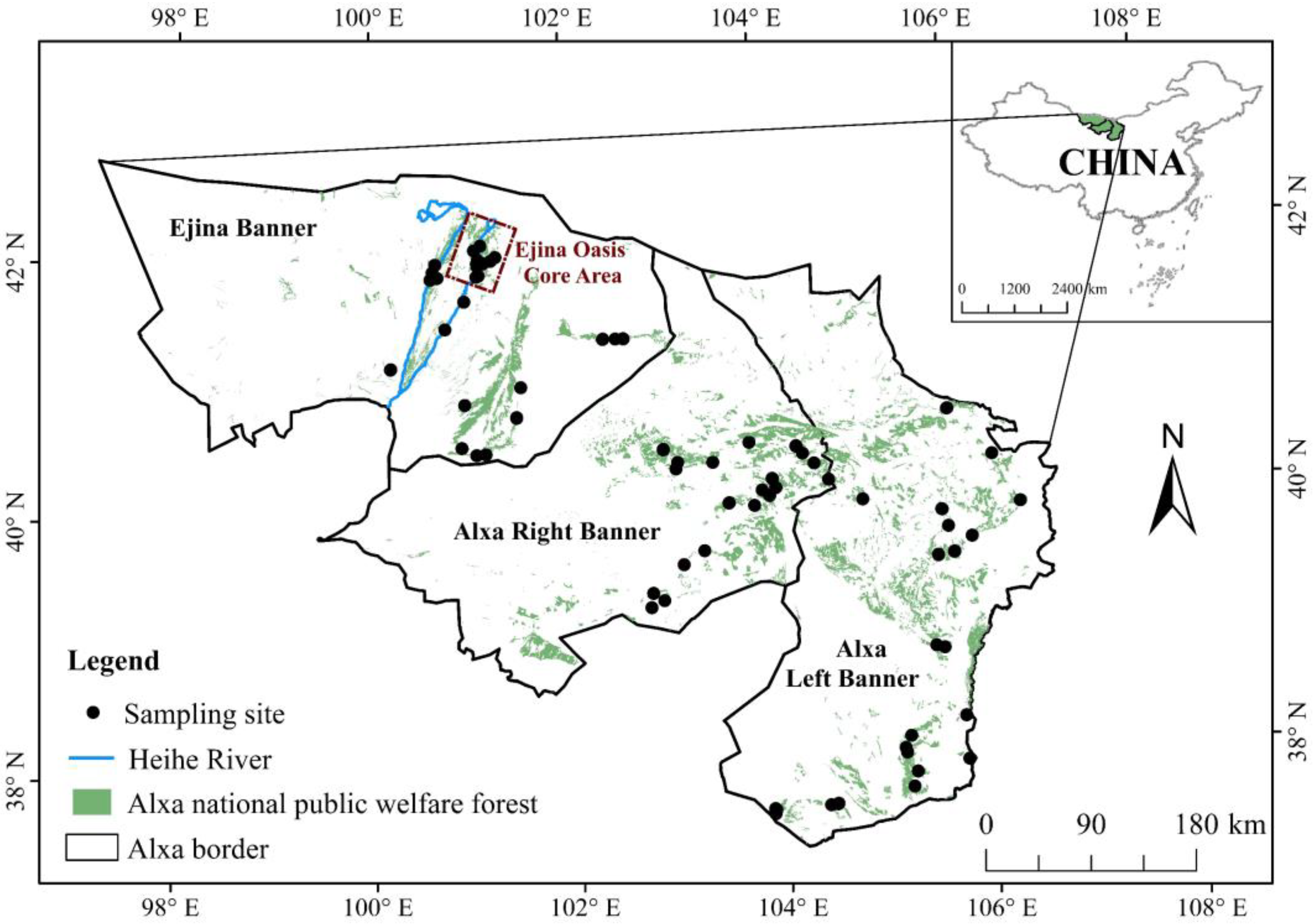
2.1. Description of the Study Area

Alxa national public welfare forest (ANPWF) is located in the western part of the Inner Mongolia Plateau (37°24′—42°47′N, 97°10′—106°53′E), China (Figure 1). The soils in the study area are Cambisols and Solonchaks [18,19], which are loose and contain soluble salts. The annual average temperature is 6~8.5 °C, the annual precipitation is 40~200 mm, and it is mostly concentrated in summer. The annual evaporation of this area is 2000~4000 mm, which makes it a typical arid area [20]. By 2021, the area of the ANPWF was 17,140.59 km², with a desert vegetation landscape consisting of dry scrub and shrubland, with the main dominant species being Haloxylon ammodendron, Caragana korshinskii, Nitraria tangutorum, Tamarix ramosissima, and Populus euphratica. ANPWF plays an active role in improving and restoring soil quality, protecting biodiversity, and meeting ecological and social needs, serving as a natural barrier to the surrounding oasis plains and maintaining the ecological balance of the Alxa region and northern China as a whole [21]. However, due to the aridity and low rainfall, strong evaporation, and sparse vegetation in the region, an arid salt accumulation soil environmental system based on weathered crusts with high carbonate content has been formed [22].

2.2. Data Collection and Processing

2.2.1. Measured SSC Data Processing

Soil samples were collected in August 2016, 2017, 2018, 2019, and 2021. August is the summer season in the study area, when vegetation grows luxuriantly, temperatures are high, and the evaporation of soil moisture is vigorous, prompting the upward movement of soil salts and the accumulation of salts in the surface layer of the soil to a more stable stage. Due to the large extent of the study area, the vegetation and soil types are not homogeneous, and there are differences in salinity under different types of vegetation and soil conditions. In order to simulate the salinization condition of soil in the study area as realistically as possible, sampling was chosen near different types of vegetation and with different types of soil. Before sampling, according to the land use type of the study area and the results of related studies, the sample points were laid out taking into account both salinized and non-salinized soils, and according to the salinity gradient, the sample points were laid out on soils with different degrees of salinization. The area of the soil collection sample plot was 20 m × 20 m, and the collection depth was 0 to 10 cm. Three soil samples were duplicated around adjacent sampling sites and mixed well. The coordinates of each sampling site and their surrounding soil and vegetation types were recorded. After removing impurities, the collected soil samples were put into sterile bags and brought back to the laboratory, where they were dried naturally and then the samples were ground and sieved. The soil total salt was calculated after measuring the content of the eight major ions in the soil. The measured SSC data were analyzed, and the abnormal values were excluded to obtain a total of 195 sample data. The SSC of the samples was graded according to the Chinese soil salinization grading standard (HJ 964-2018): SSC < 2 g/kg as unsalinized, 2 ≤ SSC < 3 g/kg as mildly salinized, 3 ≤ SSC < 5 g/kg as moderately salinized, 5 ≤ SSC < 10 g/kg as heavily salinized, and SSC ≥ 10 g/kg as saline soil [23].

2.2.2. Remote Sensing Data Processing

In this study, the remote sensing data used were the Landsat-8 OLI data provided by the United States Geological Survey (USGS, http://earthexplorer.usgs.gov/, accessed on 10 January 2023). Landsat-8 was launched on 11 February 2013, with two sensors: Operational Land Imager (OLI) and Thermal Infrared Sensor (TIRS). The OLI provides 8 bands at a spatial resolution of 30 m and a panchromatic band at 15 m. TIRS includes two separate thermal infrared bands with a resolution of 100 m [24]. To ensure the accuracy of the inversion results, the shooting time of each remote sensing image acquired was basically the same as the field sampling time, and the specific parameters are shown in Supplementary Material (Table S1). Before the experiment, the remote sensing images were preprocessed using the radiometric calibration, atmospheric correction, mosaicing and cropping modules of ENVI 5.2 to eliminate errors caused by the sensors themselves and atmospheric scattering, etc., and the images were cropped according to the boundaries of the study area for subsequent operations.

Depending on the spectral characteristics of the features and their relationships with the bands of multispectral remote sensing data, certain bands of reflectance can be combined to highlight the target features [25]. In most cases, due to large standard deviations, the correlations between bands are weak, the data independence is strong, and there is little redundancy, so more information is obtained from the composite bands [26,27]. This study selected 16 representative salinity indices, water body indices, and vegetation indices (

Table 1. Calculation formula of the spectral index.

Spectral Index	Formula	References
Salinity index (SI-T)	SI-T = Red/NIR × 100	[6]
Salinity index (SI)	SI = $\sqrt{\mathrm{B}\mathrm{l}\mathrm{u}\mathrm{e}\times \mathrm{R}\mathrm{e}\mathrm{d}}$	[6]
Salinity index (SI1)	SI1 = $\sqrt{\mathrm{G}\mathrm{r}\mathrm{e}\mathrm{e}\mathrm{n}\times \mathrm{R}\mathrm{e}\mathrm{d}}$	[28]
Salinity index (SI2)	SI2 = $\sqrt{{\mathrm{G}\mathrm{r}\mathrm{e}\mathrm{e}\mathrm{n}}^2+{\mathrm{R}\mathrm{e}\mathrm{d}}^2+{\mathrm{N}\mathrm{I}\mathrm{R}}^2}$	[28]
Salinity index (SI3)	SI3 = $\sqrt{{\mathrm{G}\mathrm{r}\mathrm{e}\mathrm{e}\mathrm{n}}^2+{\mathrm{R}\mathrm{e}\mathrm{d}}^2}$	[28]
Salinity index (SI4)	SI4 = SWIR1/NIR	[29]
Salinity index (SI5)	SI5 = (Red − SWIR1)/(Red + SWIR1)	[30]
Salinity index (SI6)	SI6 = Blue × Red/Green	[31]
Salinity index (SI7)	SI7 = Red × NIR/Green	[31]
Brightness Index (BI)	BI = $\sqrt{{\mathrm{R}\mathrm{e}\mathrm{d}}^2+{\mathrm{N}\mathrm{I}\mathrm{R}}^2}$	[32]
Normalized difference salinity index (NDSI)	NDSI = (Red − NIR)/(Red + NIR)	[32]
Soil condition vegetation index (SAVI)	SAVI = (NIR − Red) × 1.5/(NIR + Red + 0.5)	[33]
Normalized difference vegetation index (NDVI)	NDVI = (NIR − Red)/(NIR + Red)	[34]
Difference vegetation index (DVI)	DVI = NIR − Red	[35]
Ratio vegetation index (RVI)	RVI = NIR/Red	[35]
Salinity Remote Sensing Index (SRSI)	SRSI = $\sqrt{{(\mathrm{N}\mathrm{D}\mathrm{V}\mathrm{I}-1)}^2+{\mathrm{S}\mathrm{I}}^2}$	[36]

) widely used in the existing literature to inversely derive the SSC information in the study area. Band operations were performed in the ENVI 5.2 software according to the calculation formulas of each spectral index, the generated spectral index grayscale maps were matched with the actual soil salt points through geographic coordinates, and the spectral index values of each sampling point were extracted in ArcGIS 10.6 software.

2.2.3. Meteorological Data

Five variables, namely average precipitation (Pre), average temperature (Tem), average actual evapotranspiration (ETa), average wind speed (Win), and elevation (DEM) during the rainy season, were selected to investigate the extent of their influence on soil salinity. Among them, precipitation and temperature data were obtained from the ERA5-Land dataset published by the European Centre for Medium-Range Weather Forecasts (https://cds.climate.copernicus.eu/cdsapp#!/dataset/reanalysis-era5-land-monthly-means?tab=overview, accessed on 10 January 2023), both with a spatial resolution of 0.1° × 0.1° for the raw data. The actual evapotranspiration was obtained from the GLEAM data set (https://www.gleam.eu/, accessed on 10 January 2023) with a spatial resolution of 0.25° × 0.25°. Wind speed data were obtained from the National Center for Environmental Information (NCEI) under the National Oceanic and Atmospheric Administration (NOAA) (https://www.ncei.noaa.gov/data/global-summary-of-the-day/archive/, accessed on 10 January 2023), and the raw data downloaded from the NCEI website were the daily average wind speed values recorded at each station. The inverse distance-weighted interpolation method was used to obtain the daily average wind speed raster map in the study area, and then the monthly average wind speed was calculated from the daily average wind speed values. DEM data were obtained from the Shuttle Radar Topography Mission (SRTM; https://www2.jpl.nasa.gov/srtm/, accessed on 10 January 2023). Since the spatial resolution of the remote sensing images used in this study was 30 m, the raster data used, such as precipitation, temperature, evapotranspiration, and DEM data, were resampled to a spatial resolution of 30 m to minimize the error in the inversion process.

2.3. Research Methods

2.3.1. Salinity Inversion Model Construction

All soil data collected from 2016 to 2021 and their corresponding sensitive spectral indices were used as a dataset for building the SSC inversion model, which was randomly divided into a training set and a test set in a ratio of 3:1. The measured SSC data were the dependent variable y, and the spectral indices related to SSC were the independent variable x. Five soil salinity inversion models, namely Multiple Linear Regression (MLR), Partial Least Squares Regression (PLSR), Support Vector Machine (SVM), Random Forest (RF), and Convolutional Neural Networks (CNN), were trained with the data from the training set. All five methods were implemented in Python 3.9.

(1)

Multiple Linear Regression (MLR)

MLR is commonly used to predict the dependent variable via the optimal combination of multiple independent variables together, based on the linear relationship between the independent and dependent variables, and is commonly used for salt inversion [37,38].

(2)

Partial Least Squares Regression (PLSR)

PLSR combines the features of principal component analysis, correlation analysis, and linear regression analysis in the modeling process, can include multiple response variables at the same time, and can eliminate the covariance among the participating predictor variables to a certain extent [39], and is suitable for situations where the number of predictor points is greater than the number of observation points [40].

(3)

Support Vector Machine (SVM)

SVM is a kernel function-based learning method widely used for pattern classification and model regression and is a nonlinear modeling technique [41,42]. In the modeling process, the SVM algorithm maps the raw input data to a high-dimensional feature space using kernel functions, and it can efficiently handle a relatively small amount of sample data. The kernel function type used in this study was “liner”, with a penalty factor of 1.0 and a residual convergence threshold of 0.001.

(4)

Random Forest (RF)

RF can calculate the importance of variables and simulate complex interactions among a large number of predictor variables, usually providing higher accuracy predictions [43,44], and it has been increasingly used in soil salinity studies in recent years [45]. The specific parameters of the model in this study were set as follows: the number of decision trees was 186, criterion = ‘mae’, min_samples_leaf = 3, max_depth = 2.

(5)

Convolutional Neural Network (CNN)

CNN is a neural network specifically designed to process data with known topology, which mainly contain convolutional and pooling layers [46]. In this study, the CNN prediction model was built using a network structure with one convolutional layer, one pooling layer, and three fully connected layers. In the prediction model, the convolutional layer automatically extracts the local features and patterns of the input data by sliding the convolutional kernel over the input data, which enables the model to capture the relationship between the input and output effectively. The pooling layer is responsible for the dimensionality reduction in the output of the convolutional layer to reduce the computational complexity and improve the generalization ability of the model. Finally, a three-layer fully connected layer adds depth to the model and enhances the nonlinear fitting capability to output the inverse results. The specific parameters of the model are shown in

Table 2. CNN model parameters.

Layer	Parameters
Conv1D	filters = 14, kernel_size = 2
AveragePool	pool_size = 2
Dense_1	units = 48
Dense_2	units = 24
Dense_3	units = 1
Total parameters = 2131

:

The accuracy and stability of each model were compared in the test set using assessment metrics such as coefficient of determination (R²), normalized root mean square error (NRMSE), and relative analysis error (RPD). The closer R² was to 1 and the closer NRMSE was to zero, the higher the accuracy of the model. When RPD < 1.4, the model was considered unreliable; when 1.4 < RPD < 2.0, the model was considered more reliable; and when RPD > 2.0, the model was considered to have high reliability [47]. R², NRMSE, and RPD were calculated using the following equations:

$$R^2=1-\frac{{\displaystyle {\sum }_{i=1}^n({\stackrel{\wedge }{y}}_i-y_i{)}^2}}{{\displaystyle {\sum }_{i=1}^n(y_i-\stackrel{-}{y}{)}^2}}$$

(1)

$$RMSE=\sqrt{\frac{{\displaystyle {\sum }_{i=1}^n(\stackrel{\wedge }{y_i}-y_i{)}^2}}{n}}, NRMSE=\frac{RMSE}{\max (y_i)-\min (y_i)}$$

(2)

$$RPD=\frac{SD}{RMSE}$$

(3)

where y_i is the measured soil salinity; $\stackrel{-}{y_i}$ is the mean of the measured soil salinity; $\stackrel{\wedge }{y_i}$ is the soil salinity of model prediction; n is the number of samples; and SD is the standard deviation of the measured soil salinity.

2.3.2. Geodetector Model

The geodetector model can be used to measure the quantitative relationship between the dependent and the analyzed variables in our research. It is a tool to detect spatial variability and reveal its driving factors, allowing it to quantify the influence of individual factors and the interactions of multiple factors [48]. By calculating and comparing the q values of single factors, as well as the q values of different factors superimposed on each other, the geodetector can determine whether there is an interaction between the influencing factors and the strength of their interaction. The geodetector consists of four detectors, including an interaction detector, ecological detector, factor detector, and risk detector. The factor detector and interaction detector were used in this study to explore the influencing factors of SSC variation.

(1)

Factor detector: it is used to detect the spatial variance of the dependent variable Y (SSC) and the magnitude of the spatial variance of the independent variable X (each influence factor) on Y, expressed as q:

$$q=1-\frac{{\displaystyle {\sum }_{h=1}^L{N}_h{\mathit{\sigma }}_h^2}}{N{\mathit{\sigma }}^2}=1-\frac{SSW}{SST}$$

$$SSW={\displaystyle {\sum }_{h=1}^L{N}_h{\mathit{\sigma }}_h^2}, SST=N{\mathit{\sigma }}^2$$

(4)

where h =1, …, and L is the classification of variable Y or factor X. N_h and N represent the number of units in class h and the whole area, respectively. ${\mathit{\sigma }}_h^2$ and ${\mathit{\sigma }}^2$ are the variances of Y for class h and the whole region, respectively. SSW and SST are within sum of squares and total sum of squares, respectively. The range of q is [0, 1], and the larger the value of q, the stronger the influence of X on the spatial variance of Y.

(2)

Interaction detector: used to identify the interactions between different factors and assess whether two factors strengthen or weaken the explanatory power of the dependent variable.

The independent variables entered in the geodetector should be typed quantities, and if they are numerical quantities, they need to be discretized. In this study, the continuous data of five influencing factors (Pre, Tem, ETa, Win, and DEM) were classified into five categories using the Natural Break method (a method of partitioning spatial data, which is based on the principle of grouping the data in the most appropriate way so that the differences between each group are maximized and the differences within the group are minimized) in Arcmap 10.6 software. A fishnet tool was then created with a cell size of 30 m × 30 m. Grid points were randomly generated as sampling points for matching the Y-value (SSC) with the X-values (the five influencing factors). The values of each raster layer at each point were extracted and entered into the geodetector, and the software was run to obtain quantitative relationships between SSC and drivers.

3. Results

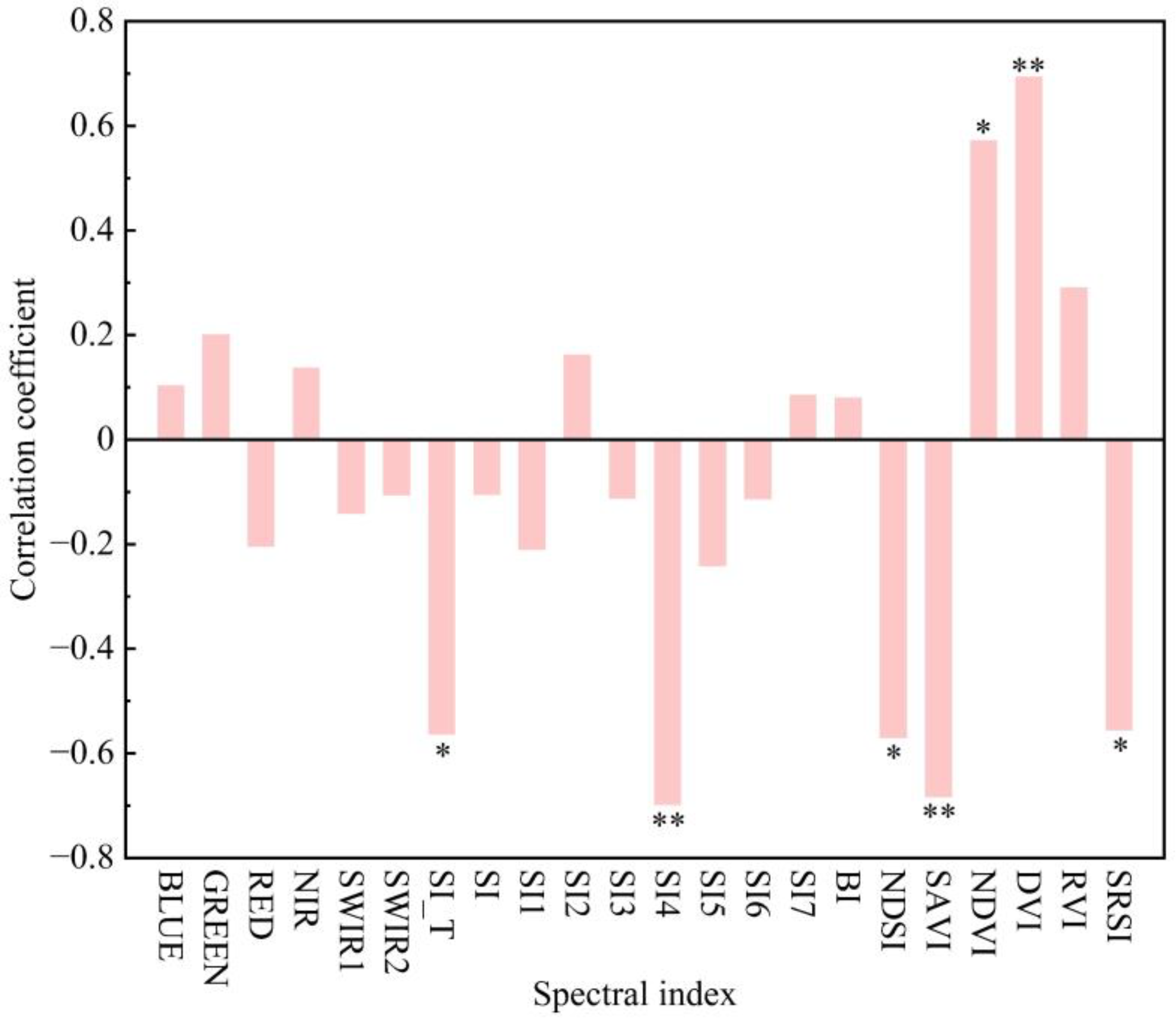
3.1. Spectral Index Preference

Although spectra do not directly reflect SSC, they can be used indirectly to indicate SSC [8]. In this study, we correlated several indicators proposed in the existing literature for assessing SSC with the actual measured SSC in samples. From Figure 2, the correlations between the spectral reflectance of single bands and SSC were all low, and among the spectral indices combined into multiple bands, SI4, SAVI, and DVI were highly significantly correlated with SSC (p < 0.01). These spectral indices were more capable of predicting soil salinity. SI-T, NDSI, NDVI, and SRSI were significantly correlated with SSC (p < 0.05). Therefore, seven spectral indices, SI-T, SI4, NDSI, SAVI, NDVI, DVI, and SRSI, were selected to participate in the construction of the prediction model in this study.

3.2. Model Selection

The seven selected sensitive spectral indices were used as independent variables, while the sample data served as dependent variables to construct MLR, PLSR, SVM, RF, and CNN models, respectively, and then compare the accuracy of several models.

Table 3. Model accuracy comparison.

Modeling Method	R2	NRMSE	RPD
CNN	0.745	0.090	1.979
RF	0.650	0.105	1.690
SVM	0.412	0.136	1.304
PLSR	0.622	0.109	1.627
MLR	0.597	0.113	1.575

shows the prediction accuracy of five models, with CNN showing the highest simulation accuracy (R² = 0.745, NRMSE = 0.090, RPD = 1.979), followed by RF and PLSR (R² above 0.6 and RPD greater than 1.6). MLR performed moderately well, with an R² of 0.597 and an RPD of 1.575. SVM showed the worst simulation accuracy. Thus, CNN had higher accuracy in the inversion of SSC compared with the other four models, and this study used CNN to construct the model and perform a spatial simulation of SSC for the ANPWF.

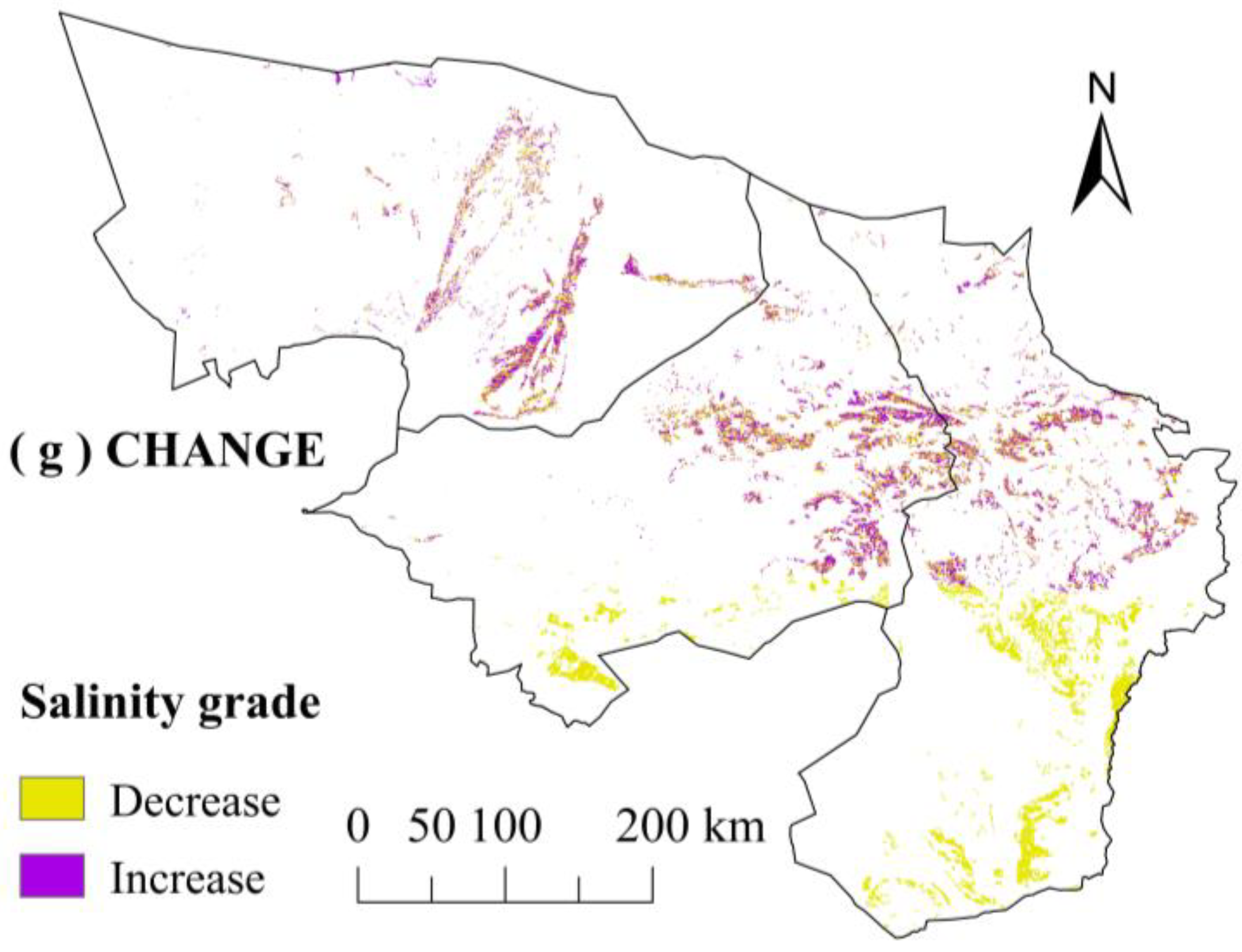
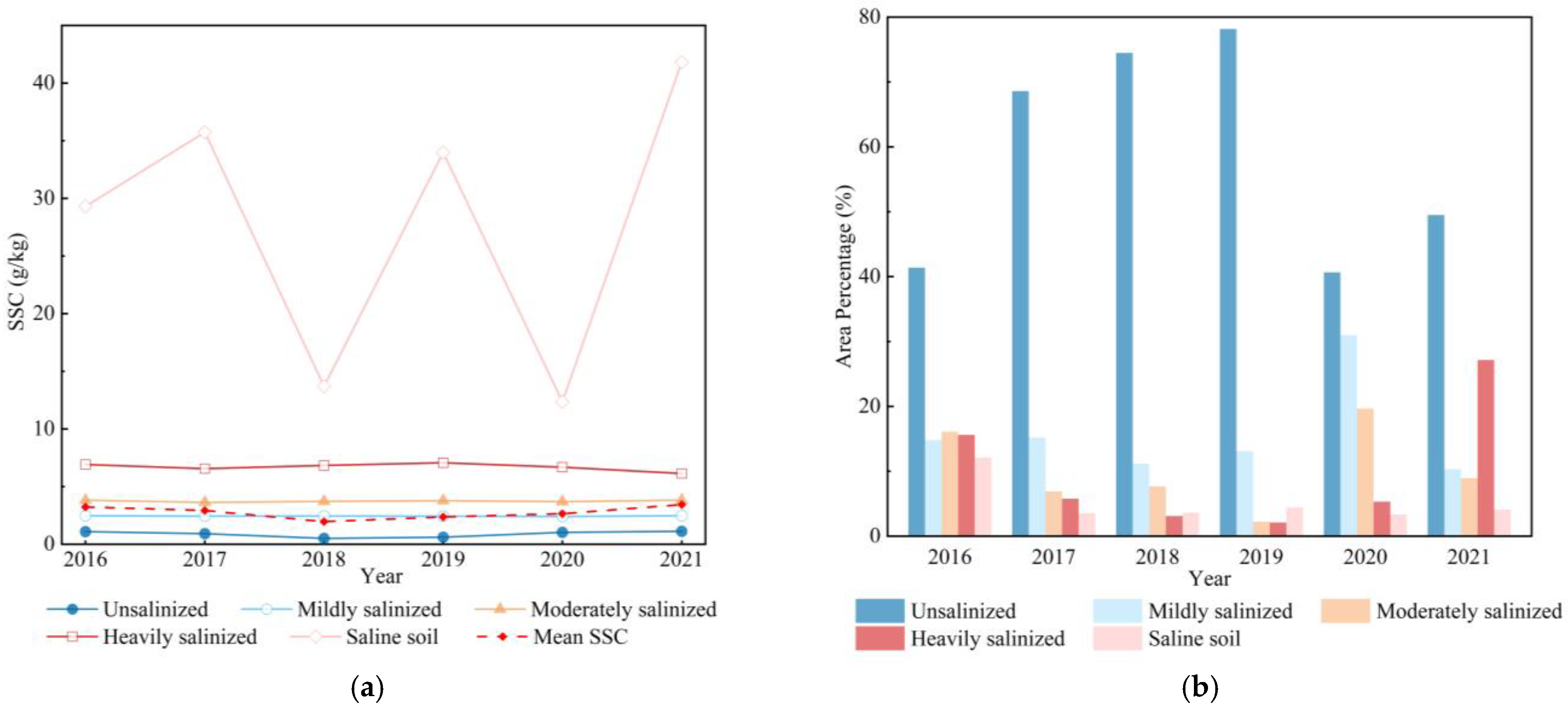
3.3. Spatial and Temporal Variations of SSC

ArcGIS 10.6 software was used to create a fishnet in the study area, extract a large number of point data, and input it into the trained CNN model to obtain the predicted values of SSC. The data points output from the model were rasterized to obtain the SSC distribution simulation map. From the overall spatial distribution of SSC in the study area from 2016 to 2021 (Figure 3a–f), the high-value areas of salinity (SSC > 5 g/kg) were mainly distributed in the northern part of Ejina Banner, followed by the eastern part of Alxa Left Banner, and the low-value areas of salinity were mainly distributed in the southeastern part of the area. From the spatial variation of SSC (Figure 3g), the areas with a significant increase in SSC were mainly distributed in Ejina Banner, the northern part of Alxa Right Banner and Left Banner, while the areas with a significant decrease in SSC were mainly concentrated in the southern part of Alxa Right Banner and Left Banner, and scattered in Ejina Banner, Right Banner, and the northern part of Left Banner.

From the annual soil salt content (

Table 4. Descriptive statistics of SSC.

Year	Number of Samples	Maximum (g/kg)	Minimum (g/kg)	Mean (g/kg)	Standard Deviation (g/kg)	Cv
2016	40	25.35	0.33	2.54	5.43	2.14
2017	42	32.53	0.19	2.55	6.10	2.39
2018	42	42.47	0.28	2.25	6.59	2.93
2019	34	41.75	0.24	2.92	8.30	2.84
2021	38	37.72	0.18	3.06	7.65	2.50

), from 2016 to 2021, the mean values of measured SSC were all between 2 and 3 g/kg, which is considered to be mildly salinized. However, the SSC increased in 2021, reaching an average value of 3.06 g/kg, which was considered to be moderately salinized. The coefficient of variation (C_v) reflects the dispersion degree of sample data. The C_v values of SSC from 2016 to 2021 were more than 1, which is considered high-variability, suggesting that the distribution of SSC was not concentrated and that soil salinity may be influenced spatially by a variety of factors, making SSC vary widely in different areas; the soil may have very high salinity in some areas.

Figure 4 shows the variations of SSC obtained from model inversion. In terms of interannual variation in salinity classes (Figure 4a), saline soil exhibited dramatic, fluctuating changes. From 2016 to 2021, the mean values of SSC for saline soil increased overall, with the highest value occurring in 2021 at 41.833 g/kg and the lowest value occurring in 2020 at 12.366 g/kg. The mean values of SSC for all other salinity grades remained stable. An analysis of the average soil salinity for each year from 2016 to 2021 revealed a non-linear trend, with a decrease followed by an increase in mean salinity over time. The lowest value was recorded in 2018, measuring 1.957 g/kg, falling within the unsalinized grade. Conversely, the highest value was recorded in 2021, measuring 3.434 g/kg, indicating a state of moderate salinization.

Figure 4b illustrates the percentages of area in different salinity grades of soil from 2016 to 2021. The area of unsalinized soils increased and then decreased. The area of both mildly and moderately salinized soils displayed a non-linear pattern of change, with an initial decrease, followed by an increase, and then another decline. The area of heavily salinized soils decreased from about 15% of the ANPWF area in 2016 to about 2% in 2019, and then increased abruptly to about 27% of the area in 2021. The change in the area of saline soil was relatively small and remained stable after decreasing from about 12% to about 4% of the ANPWF area from 2016 to 2017. Overall, from 2016 to 2019, there was a shift, mainly from heavily salinized and above grades to the unsalinized grade, and from 2020 onwards the shift between different grades of salinized soils went from the unsalinized grade to moderately and heavily salinized grade soils.

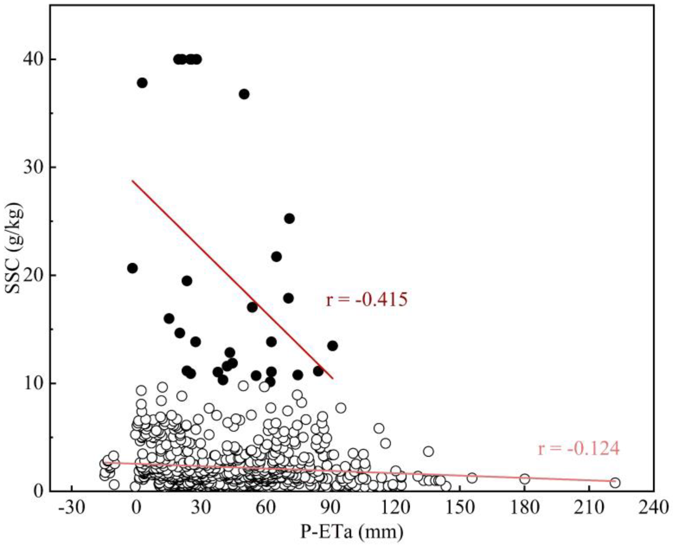
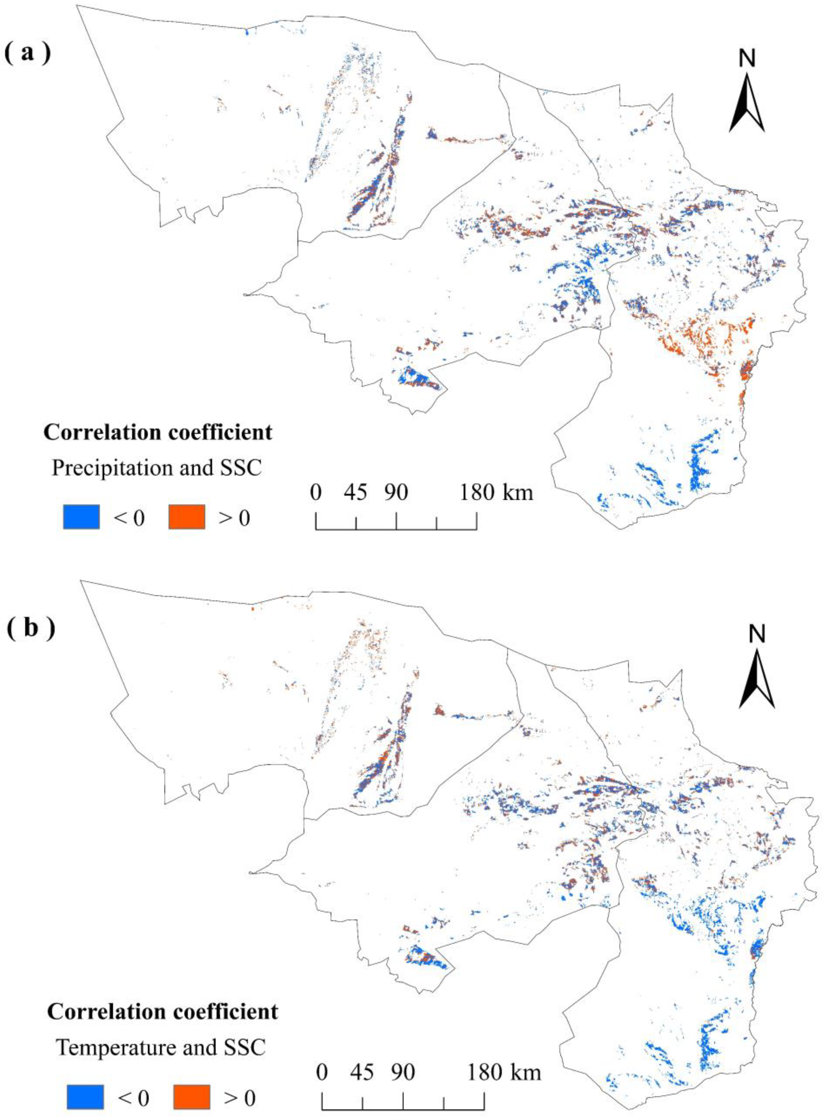
3.4. Driving Factors of SSC

To investigate the influence of different factors on SSC in the ANPWF, the single factor q values were first analyzed to identify the dominant driver. As can be seen from Figure 5, the driving magnitude of each driver on SSC was ranked as actual evapotranspiration (0.574) > temperature (0.522) > precipitation (0.491) > DEM (0.344) > wind speed (0.102). This result indicated that actual evapotranspiration was the main determinant affecting SSC, followed by temperature and precipitation, while DEM and wind speed only showed a weak influence. In general, the formation of soil salinity was influenced by several factors, so it is also crucial to explore the interaction of different influencing factors. The result showed that the combined effect of two influencing factors was greater than that of the single factor on soil salinization, where DEM and wind speed, precipitation and wind speed together showed a non-linear enhancement (interaction q value greater than the sum of the two individual q values), except that all other factors together showed a bivariate enhancement (interaction q value greater than the maximum of the individual q values). These findings indicate that the process of soil salinity accumulation is the result of the interactions and constraints between multiple factors.

The process of soil salinization is largely influenced by a range of environmental factors, with climatic conditions being one of the most significant determinants. Combining the results of this study and existing studies, the main influencing factors, such as actual evapotranspiration, precipitation and temperature, were selected to further investigate their correlation with SSC. The difference between precipitation and actual evapotranspiration represented the moisture surplus and deficit status, with a difference greater than 0 indicating a moisture surplus and a difference less than 0 indicating a moisture deficit. From Figure 6, SSC tended to decrease as P–ETa increased. When SSC was below 10 g/kg, SSC showed a weak negative correlation with P–ETa, while when SSC reached the saline soil grade, SSC showed a significant negative correlation with P–ETa (p < 0.05). This result suggests that salinity exhibits a heightened sensitivity to moisture when the moisture residual is minimal, and the soil exhibits high salinity values. Conversely, as the moisture residual amplifies, the salinity typically reduces, and its correlation with moisture becomes attenuated. The reason for this phenomenon may be that when the moisture is at a deficit, the salts in the soil accumulate heavily on the soil surface due to strong evaporation rising to the surface with capillary water and exhibiting high salinity, while as the moisture conditions become better, the salts in the soil are diluted by leaching and the surface soil salinity is at a low level. Therefore, high-salinity areas with poor moisture conditions are priority areas for ANPWF monitoring and protection, while low-salinity areas with better moisture conditions are more suitable for vegetation growth.

Based on the fishnet tool created in 2.3.2., ArcGIS 10.6 software was utilized to extract partial values to points in the raster maps of average precipitation (Pre), average temperature (Tem), and average soil salt content (SSC) for the rainy season from 2016 to 2021. Figure 7 illustrates the nonlinear behavior of SSC with respect to precipitation and temperature. Specifically, as precipitation increases, SSC undergoes an initial rapid decline, followed by a more gradual decrease after reaching a threshold of approximately 40 mm (Figure 7a). Conversely, SSC exhibits a measured rise with increasing temperature, accelerating notably beyond 28 °C (Figure 7b). These observations highlight the sensitivity of SSC to climatic variations, with noticeable change upon reaching certain moisture and thermal thresholds.

To identify the regions where climate factors have a strong effect on soil salinity, the spatial distribution of the correlation between SSC and Pre and Tem was plotted on a raster cell scale (Figure 8). Overall, temperature exhibited a positive correlation with SSC, with a mean value of 0.08. This relationship was primarily observed in the northern region of Ejina Banner and the central region of Alxa Left Banner. Precipitation was found to have a negative correlation with SSC, with an average coefficient of −0.07. This relationship was observed primarily in Ejina Banner, eastern Alxa Right Banner, and southern Alxa Left Banner. Combined with the spatial distribution results in Figure 3, the high-value area of SSC was also mainly concentrated in Ejina Banner, which is arid with little rain and strong evaporation, proving that climatic conditions are an essential factor affecting the dynamics of SSC in the study area.

4. Discussion

4.1. Model Uncertainty Analysis

In this paper, five models were developed to simulate soil salinity conditions in ANPWF by combining remote sensing data. Machine learning methods were overall better than traditional statistical methods, which was consistent with most algorithm comparison studies [49,50]. In previous studies on soil salinity inversion, algorithms such as RF and ANN were mostly used, and fewer studies used CNN because the selection of specific models was limited by different study areas and the number of samples, among other things [12]. In this paper, CNN showed the best simulation results (R² = 0.745, NRMSE = 0.090), indicating that CNN has significant potential in assessing soil salinity.

Although the inversion effect of the ANPWF soil salinity in this paper achieved a certain accuracy, errors are inevitable in the model training process, and the selection of samples and remote sensing data may also affect the model’s accuracy. In addition, the remote sensing monitoring of soil salinity is also affected by different surface vegetation, soil moisture levels, and soil texture, and the inversion of soil salinity using only the spectral index as the independent variable still faces accuracy problems in time and space scales. In the subsequent study, we can consider adding some environmental factors affecting the formation of salinized soil in the modeling process to achieve the more accurate monitoring of a large area. Secondly, it is also worth exploring whether higher accuracy can be achieved in other areas using the inversion model developed in this study.

4.2. Mechanism of Salinity Change

From the SSC simulation results, it can be concluded that the areas with serious salinization in the study area were mainly distributed in the lower reaches of the Heihe River in the northern part of Ejina Banner, and the distribution of salts was more concentrated along both sides of the river, which was basically in line with the results of some scholars on the spatial pattern of soil salinity in the region [51,52]. Climate is an important factor contributing to higher soil salinity in this region. According to existing studies, under arid climatic conditions, highly saline horizons rich in calcite, gypsum, manganese, and other minerals are deposited, and these minerals undergo biological, physical, and chemical weathering, and the salinization of soil-forming matrices constitutes the basis for the high soil salinity in the region [53]. Changes in precipitation and temperature, on the other hand, contribute to the constant changes in salinity levels, and according to the monitoring data from the meteorological stations, the average precipitation in the study area showed a trend of increasing and then decreasing from 2016 to 2021, with the highest amount of precipitation in 2018, and the temperature was lower relative to the other years of the study, and thus the results of the study demonstrated a gradual decrease in the SSC from 2016 to 2018, and then a rebound in 2019. Spatially, the variation in precipitation in the study area showed a decreasing trend from southeast to northwest, and the temperature showed a decreasing and then increasing trend from east to west. The SSC showed a corresponding distribution pattern because the lower the precipitation, the higher the temperature and the easier it was for the surface to accumulate salts.

In addition, the topography is also a factor that affects SSC [54,55]. The lower reaches of the Heihe River are the water and salt drainage area for the entire watershed. The passage of a river through densely populated areas, such as midstream and downstream regions, results in the dissolution of numerous soluble salts in the watercourse. These salts are subsequently recharged into the groundwater surrounding the riverbanks via lateral seepage. The groundwater continuously dissolves the salt ions in the surrounding bedrock during the flow process, increasing its mineralization, so the soil along the riverbank area also has high salinity. Closer to the tail end of the river, the SSC also rises rapidly due to the decrease in surface water volume and the increase in mineralization as the groundwater continuously dissolves salts in the bedrock [56].

The uneven distribution of water resources also contributes to severe soil salinization in the lower reaches of the Heihe River. The mountain forests, scrub and grasslands in the upper reaches of the river consume a large amount of water, the irrigation area in the middle reaches continues to expand and a large number of water conservancy facilities have been built, all of which have led to a decrease in water volume in the lower reaches of the river, the gradual shrinkage of the terminal lake, and an increase in lake and groundwater mineralization [57]. When the groundwater level was high, there was active salt accumulation. After the water table dropped to a threshold depth, the salts remained in the soil and became residual salt accumulation, so the downstream SSC has been at a high level for many years.

4.3. Impacts of Soil Salinity Change on the ANPWF

As a natural protective forest in the desert area, the vegetation in the ANPWF plays a vital role in maintaining the integrity and stability of the surrounding ecosystem. However, the accumulation of soil salinity often affects the healthy growth of vegetation. Many studies have found that plant species composition, distribution patterns, cover, and diversity characteristics vary with changes in soil salinity. For example, Goto et al. [58] showed that NDVI decreased in plant areas affected by salinization. Allbed et al. [59] found a robust negative correlation between NDVI and the salinity index, concluding that changes in vegetation zones are closely related to changes in soil salinity. In addition, soil salinity is the main influencing factor for plant diversity in arid zones [60], high concentrations of salinity in the soil inhibit plant growth, and salt-intolerant species are eliminated in high salinity gradients, ultimately leading to a decrease in the plant diversity index with increasing salinity [61]. According to the results of this study, the SSC in the northern areas of Ejina Banner, Alxa Left Banner, and Right Banner have a tendency to increase, and if the salinization condition in these areas continues to deteriorate, it will affect the growth of vegetation in forest areas and will not be conducive to the role of protective forests. SSC in the southern parts of Alxa Right Banner and Left Banner had a tendency to improve from 2016 to 2021, and if the salinization condition can continue to improve, it may allow vegetation to recover, creating benign soil–vegetation feedback. ANPWF is a protective forest in an arid desert ecosystem, and changes in vegetation structure due to salinity changes may in turn lead to changes in ecosystem function. Therefore, timely salt monitoring and the proper management of salt conditions are essential to ensure the ecological balance and sustainable development of desert natural protected forest areas. In this paper, we quantitatively assessed the surface salinity in the forest area, but further research is needed on the interaction relationship between salinity change and vegetation.

5. Conclusions

In this study, we firstly inversed and evaluated the salinity dynamics of ANPWF from 2016 to 2021 using remote sensing data; secondly, we quantified the factors affecting SSC; and finally, we explored the ecological impacts caused by soil salinity on desert forest areas. By comparing the five models, the CNN model performed the best in soil salinity inversion, with a simulation accuracy of 0.745, indicating that remote sensing inversion based on machine learning methods is an effective tool for monitoring SSC. From the SSC simulation results, it can be concluded that the areas with severe salinization were mainly distributed in the northern part of Ejina Banner, and from 2016 to 2021, the SSC showed an overall increasing trend, and the area of soils affected by salinization gradually expanded, which indicates that the soil salinization in the study area is still further aggravated. Combined with the monitoring data from meteorological stations, the climatic conditions of drought with low precipitation and strong evaporation are the dominant factors contributing to the accumulation of salts. In this study, it was found that soil salinity was at a high level when the precipitation was lower than 40 mm and the temperature was higher than 28 °C. This study will deepen our understanding of soil salinity dynamics in arid environments and reveal the factors affecting soil salinity changes in desert natural protected forests, providing a reference for forest area protection and management.

References

1. Tian, F.; Hou, M.; Qiu, Y.; Zhang, T.; Yuan, Y. Salinity stress effects on transpiration and plant growth under different salinity soil levels based on thermal infrared remote (TIR) technique. Geoderma 2020, 357, 113961. [Google Scholar] [CrossRef]
2. Hassani, A.; Azapagic, A.; Shokri, N. Global predictions of primary soil salinization under changing climate in the 21st century. Nat. Commun. 2021, 12, 6663. [Google Scholar] [CrossRef] [PubMed]
3. Singh, A. Soil salinization management for sustainable development: A review. J. Environ. Manag. 2021, 277, 111383. [Google Scholar] [CrossRef] [PubMed]
4. Yang, X.; Ali, A.; Xu, Y.; Jiang, L.; Lv, G. Soil moisture and salinity as main drivers of soil respiration across natural xeromorphic vegetation and agricultural lands in an arid desert region. Catena 2019, 177, 126–133. [Google Scholar] [CrossRef]
5. Mougenot, B.; Pouget, M.; Epema, G. Remote sensing of salt affected soils. Remote Sens. Rev. 1993, 7, 241–259. [Google Scholar] [CrossRef]
6. Allbed, A.; Kumar, L.; Aldakheel, Y. Assessing soil salinity using soil salinity and vegetation indices derived from IKONOS high-spatial resolution imageries: Applications in a date palm dominated region. Geoderma 2014, 230, 1–8. [Google Scholar] [CrossRef]
7. Rao, B.; Sankar, T.; Dwivedi, R.; Thammappa, S.; Venkataratnam, L.; Sharma, R.; Das, S. Spectral Behavior of Salt-Affected Soils. Int. J. Remote Sens. 1995, 16, 2125–2136. [Google Scholar] [CrossRef]
8. Hu, J.; Peng, J.; Zhou, Y.; Xu, D.; Zhao, R.; Jiang, Q.; Fu, T.; Wang, F.; Shi, Z. Quantitative Estimation of Soil Salinity Using UAV-Borne Hyperspectral and Satellite Multispectral Images. Remote Sens. 2019, 11, 736. [Google Scholar] [CrossRef]
9. Xu, L.; Wang, Q. Retrieval of Soil Water Content in Saline Soils from Emitted Thermal Infrared Spectra Using Partial Linear Squares Regression. Remote Sens. 2015, 7, 14646–14662. [Google Scholar] [CrossRef]
10. Zhang, S.; Zhao, G.; Wang, Z.; Xiao, Y.; Lang, K. Remote sensing inversion and dynamic monitoring of soil salt in coastal saline area. J. Agric. Resour. Environ. 2018, 35, 349–358. [Google Scholar] [CrossRef]
11. Morgan, R.S.; Abd El-Hady, M.; Rahim, I.S. Soil salinity mapping utilizing sentinel-2 and neural networks. Indian J. Agric. Res. 2018, 52, 524–529. [Google Scholar] [CrossRef]
12. Wang, N.; Xue, J.; Peng, J.; Biswas, A.; He, Y.; Shi, Z. Integrating Remote Sensing and Landscape Characteristics to Estimate Soil Salinity Using Machine Learning Methods: A Case Study from Southern Xinjiang, China. Remote Sens. 2020, 12, 4118. [Google Scholar] [CrossRef]
13. Li, X.; Qiao, M.; Zhou, S. Causes and Spatial-temporal Changes of Soil Salinization in Manasi Irrigation Region of Xinjiang Region during 1985–2014. Bull. Soil Water Conserv. 2016, 36, 152–158. [Google Scholar]
14. Connor, J.D.; Schwabe, K.; King, D.; Knapp, K. Irrigated agriculture and climate change: The influence of water supply variability and salinity on adaptation. Ecol. Econ. 2012, 77, 149–157. [Google Scholar] [CrossRef]
15. Stavi, I.; Thevs, N.; Priori, S. Soil Salinity and Sodicity in Drylands: A Review of Causes, Effects, Monitoring, and Restoration Measures. Front. Environ. Sci. 2021, 9, 712831. [Google Scholar] [CrossRef]
16. Meng, X.; Zhou, J.; Sui, N. Mechanisms of salt tolerance in halophytes: Current understanding and recent advances. Open Life Sci. 2018, 13, 149–154. [Google Scholar] [CrossRef] [PubMed]
17. Chen, Y.; Yin, L.; Bai, X. The influences of surface water-overflowing disturbance on the fluctuations of Tamarix ramosissima community in Western China. Acta Ecol. Sin. 2010, 30, 245–250. [Google Scholar] [CrossRef]
18. Zhang, W.; Xu, A.; Zhang, R.; Ji, H. Review of Soil Classification and Revision of China Soil Classification System. Sci. Agric. Sin. 2014, 47, 3214–3230. [Google Scholar]
19. IUSS Working Group WRB. World Reference Base for Soil Resources. International Soil Classification System for Naming Soils and Creating Legends for Soil Maps; World Soil Resources Reports; Food and Agriculture Organization of the United Nations: Rome, Italy, 2015. [Google Scholar]
20. Lu, Z.; Xu, D.; Zhang, X.; Zhao, Z.; Zhang, X. Impact of land use change on ecosystem services in arid desert region of Alxa. Res. Soil Water Conserv. 2019, 26, 296–302. [Google Scholar] [CrossRef]
21. Xi, H.; Feng, Q.; Cheng, W.; Si, J.; Yu, T. Spatiotemporal variations of Alxa national public welfare forest net primary productivity in northwest China and the response to climate change. Ecohydrology 2022, 15, e2377. [Google Scholar] [CrossRef]
22. Chen, X.; Duan, Z.; Luo, T. Changes in soil quality in the critical area of desertification surrounding the Ejina Oasis, Northern China. Environ. Earth Sci. 2014, 72, 2643–2654. [Google Scholar] [CrossRef]
23. HJ 964-2018; Technical Guidelines for Environmental Impact Assessment—Soil Environment. Ministry of Ecology and Environment of the People’s Republic of China: Beijing, China, 2018.
24. Sabri, E.M.; Boukdir, A.; Karaoui, I.; Arioua, A.; Messlouhi, R.; Idrissi, A.E.A. Modelling soil salinity in Oued EI Abid watershed, Morocco. E3S Web Conf. 2018, 37, 04002. [Google Scholar] [CrossRef]
25. Allbed, A.; Kumar, L. Soil salinity mapping and monitoring in arid and semi-arid regions using remote sensing technology: A review. Adv. Remote Sens. 2013, 4, 373–385. [Google Scholar] [CrossRef]
26. Chavez, P.; Berlin, G.; Sowers, L. Statistical-Method for Selecting Landsat MSS Ratios. J. Appl. Photogr. Eng. 1982, 8, 23–30. [Google Scholar]
27. Yu, R.; Liu, T.; Xu, Y.; Zhu, C.; Zhang, Q.; Qu, Z.; Liu, X.; Li, C. Analysis of salinization dynamics by remote sensing in Hetao Irrigation District of North China. Agric. Water Manag. 2010, 97, 1952–1960. [Google Scholar] [CrossRef]
28. Douaoui, A.; Nicolas, H.; Walter, C. Detecting salinity hazards within a semiarid context by means of combining soil and remote-sensing data. Geoderma 2006, 134, 217–230. [Google Scholar] [CrossRef]
29. Zhang, Z.; Song, Y.; Zhang, H.; Li, X.; Niu, B. Spatiotemporal dynamics of soil salinity in the Yellow River Delta under the impacts of hydrology and climate. J. Appl. Ecol. 2021, 32, 1393–1405. [Google Scholar] [CrossRef]
30. Bannari, A.; Guedon, A.; El-Harti, A.; Cherkaoui, F.; El-Ghmari, A. Characterization of Slightly and Moderately Saline and Sodic Soils in Irrigated Agricultural Land using Simulated Data of Advanced Land Imaging (EO-1) Sensor. Commun. Soil Sci. Plant Anal. 2008, 39, 2795–2811. [Google Scholar] [CrossRef]
31. Abbas, A.; Khan, S.; Hussain, N.; Hanjra, M.; Akbar, S. Characterizing soil salinity in irrigated agriculture using a remote sensing approach. Phys. Chem. Earth 2013, 55–57, 43–52. [Google Scholar] [CrossRef]
32. Khan, N.M.; Rastoskuev, V.V.; Sato, Y.; Shiozawa, S. Assessment of hydrosaline land degradation by using a simple approach of remote sensing indicators. Agric. Water Manag. 2005, 77, 96–109. [Google Scholar] [CrossRef]
33. Huete, A. A Soil-Adjusted Vegetation Index (SAVI). Remote Sens. Environ. 1988, 25, 295–309. [Google Scholar] [CrossRef]
34. Rouse, J. Monitoring the Vernal Advancement of Retrogradation (Green Wave Effect) of Natural Vegetation; NASA/GSFC Type III Final Report; NASA/GSFC: Greenbelt, MD, USA, 1974. [Google Scholar]
35. Bannari, A.; Morin, D.; Bonn, F.; Huete, A. A review of vegetation indices. Remote Sens. Rev. 1995, 13, 95–120. [Google Scholar] [CrossRef]
36. Alhammadi, M.; Glenn, E. Detecting date palm trees health and vegetation greenness change on the eastern coast of the United Arab Emirates using SAVI. Int. J. Remote Sens. 2008, 29, 1745–1765. [Google Scholar] [CrossRef]
37. Marshall, F.; Smith, D.; Nickerson, D. Empirical tools for simulating salinity in the estuaries in Everglades National Park, Florida. Estuar. Coast. Shelf Sci. 2011, 95, 377–387. [Google Scholar] [CrossRef]
38. Pahlavan-Rad, M.; Dahmardeh, K.; Hadizadeh, M.; Keykha, G.; Mohammadnia, N.; Gangali, M.; Keikha, M.; Davatgar, N.; Brungard, C. Prediction of soil water infiltration using multiple linear regression and random forest in a dry flood plain, eastern Iran. Catena 2020, 194, 104715. [Google Scholar] [CrossRef]
39. Nawar, S.; Buddenbaum, H.; Hill, J.; Kozak, J. Modeling and Mapping of Soil Salinity with Reflectance Spectroscopy and Landsat Data Using Two Quantitative Methods (PLSR and MARS). Remote Sens. 2014, 6, 10813–10834. [Google Scholar] [CrossRef]
40. Yu, H.; Liu, M.; Du, B.; Wang, Z.; Hu, L.; Zhang, B. Mapping Soil Salinity/Sodicity by using Landsat OLI Imagery and PLSR Algorithm over Semiarid West Jilin Province, China. Sensors 2018, 18, 1048. [Google Scholar] [CrossRef]
41. Amari, S.; Wu, S. Improving support vector machine classifiers by modifying kernel functions. Neural Netw. 1999, 12, 783–789. [Google Scholar] [CrossRef] [PubMed]
42. Diao, S.; Liu, C.; Zhang, T.; He, P.; Guo, Z.; Tu, J. Extraction of remote sensing information for lake salinity level based on SVM: A case from Badain Jaran desert in Inner Mongolia. Remote Sens. Nat. Resour. 2016, 28, 114–118. [Google Scholar]
43. Mutanga, O.; Adam, E.; Cho, M. High density biomass estimation for wetland vegetation using WorldView-2 imagery and random forest regression algorithm. Int. J. Appl. Earth Obs. Geoinf. 2012, 18, 399–406. [Google Scholar] [CrossRef]
44. Were, K.; Bui, D.; Dick, O.; Singh, B. A comparative assessment of support vector regression, artificial neural networks, and random forests for predicting and mapping soil organic carbon stocks across an Afromontane landscape. Ecol. Indic. 2015, 52, 394–403. [Google Scholar] [CrossRef]
45. Wang, J.; Ding, J.; Abulimiti, A.; Cai, L. Quantitative estimation of soil salinity by means of different modeling methods and visible-near infrared (VIS-NIR) spectroscopy, Ebinur Lake Wetland, Northwest China. PeerJ 2018, 6, e4703. [Google Scholar] [CrossRef] [PubMed]
46. Garajeh, M.; Blaschke, T.; Haghi, V.; Weng, Q.; Kamran, K.; Li, Z. A Comparison between Sentinel-2 and Landsat 8 OLI Satellite Images for Soil Salinity Distribution Mapping Using a Deep Learning Convolutional Neural Network. Can. J. Remote Sens. 2022, 48, 452–468. [Google Scholar] [CrossRef]
47. Dai, X.; Peng, J.; Zhang, Y.; Luo, H.; Xiang, H. Prediction on Soil Salt Content Based on Spectral Classifi cation. Acta Pedol. Sin. 2016, 53, 909–918. [Google Scholar]
48. Wang, J.; Xu, C. Geodetector: Principle and prospective. Acta Geogr. Sin. 2017, 72, 116–134. [Google Scholar]
49. Wang, M.; Mo, H.; Chen, H. Study on Model Method of Inversion of Soil Salt Based on Multispectral Image. Chin. J. Soil Sci. 2016, 47, 1036–1041. [Google Scholar]
50. Wang, X.; Zhang, F.; Ding, J.; Kung, H.; Latif, A.; Johnson, V.C. Estimation of soil salt content (SSC) in the Ebinur Lake Wetland National Nature Reserve (ELWNNR), Northwest China, based on a Bootstrap-BP neural network model and optimal spectral indices. Sci. Total Environ. 2018, 615, 918–930. [Google Scholar] [CrossRef]
51. Jia, Y.; Zhao, C.; Nan, Z.; Wan, Y. Spatial heterogeneity of soil salinity in groundwater-fluctuating region of the lower reaches of the Heihe River. Acta Pedol. Sin. 2008, 45, 420–430. [Google Scholar]
52. Zhang, X.; Zhou, J.; Lai, L.; Jiang, L.; Zheng, Y.; Shi, L. Spatial Characterization of Soil Water-salt and Nutrient in a Desert Riparian Area Along the Lower Reaches of Heihe River, China. Ecol. Environ. Sci. 2019, 28, 1739–1747. [Google Scholar]
53. Bai, F.; Fang, G. Characteristics and causes of soil salinization in a typical interior arid basin in northwest China-the case of Heihe River Basin. Geotech. Investig. Surv. 2008, S1, 230–235. [Google Scholar]
54. Fang, H.; Liu, G.; Kearney, M. Georelational analysis of soil type, soil salt content, landform, and land use in the Yellow River Delta, China. Environ. Manag. 2005, 35, 72–83. [Google Scholar] [CrossRef]
55. Xiao, Y.; Zhao, G.; Li, T.; Zhou, X.; Li, J. Soil salinization of cultivated land in Shandong Province, China-Dynamics during the past 40 years. Land Degrad. Dev. 2019, 30, 426–436. [Google Scholar] [CrossRef]
56. Zhao, C.; Li, S.; Feng, Z.; Shen, W. Dynamics of groundwater level in the water table fluctuant belt at the lower reaches of Heihe River. J. Desert Res. 2009, 29, 365–369. [Google Scholar]
57. Xiao, S.; Xiao, H. Influencing Factors of Oasis Evolution in Heihe River Basin. J. Desert Res. 2003, 23, 385–390. [Google Scholar]
58. Goto, K.; Goto, T.; Nmor, J.; Minematsu, K.; Gotoh, K. Evaluating salinity damage to crops through satellite data analysis: Application to typhoon affected areas of southern Japan. Nat. Hazards 2015, 75, 2815–2828. [Google Scholar] [CrossRef]
59. Allbed, A.; Kumar, L.; Sinha, P. Soil salinity and vegetation cover change detection from multi-temporal remotely sensed imagery in Al Hassa Oasis in Saudi Arabia. Geocarto Int. 2018, 33, 830–846. [Google Scholar] [CrossRef]
60. Chenchouni, H. Edaphic factors controlling the distribution of inland halophytes in an ephemeral salt lake “Sabkha ecosystem” at North African semi-arid lands. Sci. Total Environ. 2017, 575, 660–671. [Google Scholar] [CrossRef]
61. Iqbal, T. Rice straw amendment ameliorates harmful effect of salinity and increases nitrogen availability in a saline paddy soil. J. Saudi Soc. Agric. Sci. 2018, 17, 445–453. [Google Scholar]
Figure 1. The map of the study area.
Remotesensing 15 05054 g001
Figure 2. Correlation coefficient between SSC and spectral indices (* represents p < 0.05; ** represents p < 0.01).
Remotesensing 15 05054 g002
Figure 3. Spatial distribution of salinization in the ANPWF: (af) SSC simulation map from 2016 to 2021, (g) spatial variation of SSC from 2016 to 2021.
Remotesensing 15 05054 g003aRemotesensing 15 05054 g003b
Figure 4. (a) Dynamic changes in SSC, and (b) percentage of soil with different salinity grades.
Remotesensing 15 05054 g004
Figure 5. Interactive detection explanatory power (q) of various factors in the study area (* indicated non-linear enhance, no * indicated bivariate enhance).
Remotesensing 15 05054 g005
Figure 6. Relationship between moisture surplus and SSC. Solid points indicate SSC greater than 10 g/kg (salinity grade is saline soil) and hollow points indicate SSC less than 10 g/kg.
Remotesensing 15 05054 g006
Figure 7. (a) Correlation between precipitation and SSC (the fitting function is a four-term Fourier series, R2 = 0.7788) and (b) between temperature and SSC (the fitting function is a two-term exponential function, R2 = 0.9498).
Remotesensing 15 05054 g007
Figure 8. (a) Spatial correlations between precipitation and SSC, and (b) between temperature and SSC.
Remotesensing 15 05054 g008