Annual and Interannual Variability in the Diffuse Attenuation Coefficient and Turbidity in Urbanized Washington Lake from 2013 to 2022 Assessed Using Landsat-8/9

Abstract

Water clarity, defined in this study using measurements of the downwelling diffuse light attenuation coefficient (K_d) and turbidity, is an important indicator of lake trophic status and ecosystem health. We used in-situ measurements to evaluate existing semi-analytical models for K_d and turbidity, developed a regional turbidity model based on spectral shape, and evaluated the spatial and temporal trends in Lake Washington from 2013 to 2022 using Landsat-8/9 Operational Land Imager (OLI). We found no significant trends from 2013 to 2022 in K_d or turbidity when both the annual and full datasets were considered. In addition to the spring peak lasting from April through June, autumn K_d peaks were present at all sites, a pattern consistent with seasonal chlorophyll a and zooplankton concentrations. There existed no autumn peak in the monthly turbidity dataset, and the spring peak occurred two months before the K_d peak, nearly mirroring seasonal variability in the Cedar River discharge rates over the same period. The K_d and turbidity algorithms were thus each more sensitive to different sources of water clarity variability in Lake Washington.

1. Introduction

1.1. Background

Water clarity directly influences and is affected by the spatiotemporal variability in phytoplankton concentration, composition, and distribution. Additionally, rivers discharge variable amounts of sediments and colored dissolved organic matter (CDOM), resulting in optically complex underwater light fields. Several metrics of water clarity are routinely measured for monitoring lake water quality, including the downwelling diffuse light attenuation coefficient (K_d) and turbidity. K_d (m⁻¹) describes the rate of light attenuation with depth in the water column and allows for the quantification of the vertical distribution of light at or over a specific wavelength rage (λ). Turbidity is defined by the International Organization for Standardization ISO 7027 [1] using the measurement at 860 nm of 90° side-scattered light with respect to Formazin and is measured in Formazin Nephelometric Units (FNU). The relationships between turbidity, K_d, and other water clarity metrics have been discussed in detail [2,3]. Knowledge of the spatiotemporal variability in water clarity is critical for understanding not only water quality trends but also behavioral patterns at higher trophic levels [4,5,6].

Over the last decade, numerous studies have applied empirical, machine learning, and semi-analytical algorithms for retrieving metrics of optical clarity from remote-sensing reflectance (R_rs; sr⁻¹) or surface reflectance (⍴_w; unitless). Both the National Aeronautics and Space Administration (NASA) and European Space Agency (ESA) use empirical algorithms, derived using oceanic and coastal datasets, that utilize the blue-to-green ratios of R_rs and in-situ measurements to calculate K_d(490). Neural networks have also been used to derive algorithms predicting K_d(λ) from R_rs(λ) [7,8], but as for empirical algorithms, they are applicable only within the range of data used for model development. In the context of freshwater research, the authors of [9] found that a Random Forest machine learning algorithm performed better than 13 previously published empirical algorithms for predicting water clarity in 397 lakes in the northeastern United States. Alternatively, the authors of [10], with their findings revised by [11], applied radiative transfer equations in the Hydrolight software to develop semi-analytical algorithms that derive K_d(λ) as a function of inherent optical properties (IOPs) and the solar zenith angle (θ).

IOPs are often calculated from R_rs using the quasi-analytical algorithm (QAA) [12], which was derived using the wavelengths of light measured by historical ocean satellite sensors (e.g., moderate-resolution imaging spectroradiometer, MODIS) which collect data at large spatial scales (1 km resolution) appropriate for large-scale ocean studies. The authors of [13] modified the QAA for use with the Landsat-8 Operational Land Imager (OLI) data (30 m resolution) and mapped water clarity in an estuary near Xiamen City, China. This work allowed for the application of IOP-based algorithms to the Landsat time series, which measures at spatial scales relevant for research of inland water bodies.

Since then, several studies have applied IOP-based algorithms for calculation and evaluation of water clarity trends in lakes across the globe. The authors of [14] applied the QAA to Landsat-5 Thematic Mapper (TM) and Landsat-8 OLI data to evaluate water clarity trends in Lake Taihu, China from 1984 through 2019. The authors of [15] tested multiple QAA-based algorithms for calculating K_d in Lake Villarrica, Chile to evaluate long-term trends in water clarity. The authors of [16] also used the QAA to calculate IOPs which were used with contrast theory to evaluate water clarity trends in more than 270 lakes and ponds across the continental United States.

For calculation of turbidity in coastal and estuarine environments, the authors of [17] developed an IOP-based algorithm using in-situ turbidity and ⍴_w(λ) measurements. This model performed well (R² = 0.949 at 665 nm) in the southern North Sea, where turbidity ranged from 0.65 to 83.63 FNU, with a 17.98 FNU mean turbidity concentration. The authors of [18] built on this research by expanding the range of turbidity values over which this algorithm was evaluated and applied. For freshwater applications, empirical models for predicting turbidity have also been developed for analysis of large-scale water clarity patterns [19,20]. Herein, we (1) evaluated existing semi-analytical models for K_d(PAR) [10] and turbidity [17], (2) developed a regional turbidity model based on spectral shape, and (3) evaluated the spatial and temporal trends in Lake Washington from 2013 to 2022 using Landsat-8/9 OLI.

1.2. Study Area

Lake Washington, which is located east of Seattle, is the second largest natural lake in Washington state. The lake was glacially formed, with a mean and maximum depth of 33 m and 65 m, respectively. There are two major inlet tributaries: the Cedar River at the southern end and the Sammamish River at the northern tip. River inflow peaks from December through February, while the lowest flows are observed July through September. The lake outlet is a man-made ship canal that connects Lake Washington to Puget Sound, and lake retention time is 2.4 years [21].

The limnology of Lake Washington has been extensively studied since the 1950s. The recovery of lake optical clarity and water quality was highly publicized [21], and bimonthly monitoring of water quality continues today. Mean annual nitrate, ammonium, and inorganic phosphorus concentrations are 220 µg L⁻¹, 25 µg L⁻¹, and 9.1 µg L⁻¹, respectively, making the lake phosphorus limited [22]. The lake experiences annual diatom blooms from March to June when chlorophyll a concentrations average 10 µg L⁻¹, but excluding the spring bloom period, chlorophyll a concentrations remain below 4 µg L⁻¹ [22].

Lake Washington has experienced a precipitous decline in sockeye salmon Oncorhynchus nerka over recent decades. Once the largest sockeye run in the lower 48 states, the sockeye fishery declined in the 1980s [23] and was closed in 2006. Predation mortality on juvenile sockeye salmon, primarily by other fish in the lake, has been implicated as the primary cause for the population decline [24]. Fish are visual predators, so an understanding of the visual environment is critical for understanding and predicting fish behaviors and function of lake food webs. For example, changes in water clarity directly impact the encounter rate between predator and prey, which can be modeled as a function of the distance predators visibly respond to prey, termed the reaction distance [25,26,27,28,29]. These studies have revealed that reaction distance declines exponentially with declining water transparency once turbidity exceeds 1.5 FNU (1.5 NTU). Piscivorous fishes also exhibit maximum reaction distances at light intensities above approximately 20 lux declining precipitously with decreasing light intensities below that threshold distance [25,26,29]. Therefore, an understanding of the spatiotemporal variability in the underwater optical environment could have significant implications for understanding the mechanisms driving the declines in juvenile salmon survival and identifying effective restoration and recovery strategies in the Lake Washington Basin.

In pelagic habitats, different fish species will occupy different depths as functions of their unique combinations of physiological responses to thermal stratification [30,31], foraging strategies [5,32,33], and behavioral and morphological adaptations to predation risk [34,35,36]. However, these dynamics are not solely influenced by thermal or optical factors. The ecology of Lake Washington has been significantly impacted by the presence of Eurasian milfoil (Myriophyllum spicatum), hereafter referred to as milfoil, an invasive aquatic plant that established dense macrophyte beds in the majority of littoral habitats down to depths of approximately 5 m over recent decades [37]. Its presence significantly alters the environment beneath the water surface, affecting the penetration of light in nearshore regions and creating microhabitats that significantly alter the distribution of native aquatic species [38,39] via diel and depth-specific variability in hypoxia [40,41]. The growth of milfoil varies both seasonally and interannually, further adding to the complexity in the visual environment used by different fish species and life stages in Lake Washington.

2. Materials and Methods

2.1. Datasets

2.1.1. In-Situ K_d

As part of its water quality monitoring program, King County collects measurements of K_d (photosynthetically active radiation, PAR [400–700 nm]) at three sites across the lake twice monthly from March through November and monthly from December through February (Figure 1b). Data collection was conducted in accordance with the Recommended Guidelines for Sampling Marine Sediment, Water Column, and Tissues in Puget Sound [42] and the Standard Operating Procedure for water clarity field measurements [43]. A LI-193SA (LI-COR, Inc., Lincoln, NE, USA) spherical underwater sensor attached to a SBE 25-Plus Sealogger CTD (Sea-Bird Scientific, Bellevue, WA, USA) was used to collect water column data, and a QSR-2200 (Biospherical Instruments Inc., San Diego, CA, USA) sensor was placed above the deck of the Sound Guardian to obtain surface PAR, which was used to standardize the in-water measurements. Measurements were recorded at a rate of 2 Hertz and interpolated to final values that represent 0.5 m depth increments. Measurements collected in the upper 2 m were removed from the analysis because data were consistently unrealistic (e.g., negative), and the surface water column (0–2 m) was assumed to be uniform and equal to K_d calculated from the 2–2.5 m depth layer. Light profiles were measured within +/− 4 h of the Landsat-8/9 overpass time at every site.

The layer-averaged diffuse attenuation coefficient, K_d(PAR; m⁻¹), was calculated as follows:

$${\mathit{K}}_{\mathit{d}}=\frac{\mathbf{1}}{{\mathit{z}}_{\mathbf{2}}-{\mathit{z}}_{\mathbf{1}}}\mathbf{\times }\mathit{l}\mathit{n}\frac{{\mathit{E}}_{\mathit{d}}\left({\mathit{z}}_{\mathbf{1}}\right)}{{\mathit{E}}_{\mathit{d}}\left({\mathit{z}}_{\mathbf{2}}\right)}$$

(1)

where E_d(z) is the downwelling irradiance measured using the LI-193SA at depth z. We accounted for the vertical structure in K_d and calculated the overall surface reflectance, including the signal contribution down to two optical depths according to [44]. Data collected at solar zenith angles greater than 80° were removed from the analysis.

2.1.2. In-Situ Turbidity

King County collects daily measurements of turbidity from a water quality profiling buoy (Figure 1b) [45]. Surface data collected using a YSI EXO² sensor (YSI Inc., Yellow Springs, OH, USA) from 2018 to 2022 and within +/− 4 h of Landsat-8/9 overpass time were used for model development. The instrument records turbidity between 0 and 4000 FNU, with an accuracy of 0.3 FNU or +/− 2% of the reading, whichever is greater. The majority of these data were not collected concurrently with E_d(z), so data collected in the upper 1 m were averaged for this analysis (i.e., no correction was made to account for the signal coming from below the surface).

Turbidity data were also independently collected as part of this project from 2021 to 2022 using a YSI 6600V2 sonde at four sites across the lake coincident with satellite overpass days (Figure 1b). The instrument records turbidity between 0 and 1000 NTU, with an accuracy of 0.3 NTU or +/− 2% of the reading. YSI’s turbidity sensors have historically followed the ISO 7027 method, so here NTU is comparable to FNU [46]. The sonde was submerged for a few minutes before data collection, allowing the sensors to reach the ambient temperature. As for the King County turbidity dataset, surface measurements only were used.

2.1.3. In-Situ Surface Reflectance

An ASD field spectrometer (Malvern PANalytical, Boulder CO) equipped with an 8° foreoptic for the selected wavelength rage of 400–900 nm was used to measure in-situ surface reflectance, ⍴_w(λ). Spectra were measured at 85 total stations on four separate days (6 July 2023, 15 August 2023, 16 August 2023, 8 September 2023). These data were used to qualitatively assess and control the OLI data before model evaluation and development. Radiance data were collected using the ‘above-water method’ with zenith and azimuth angles equal to 35–40° and 135°, respectively [47]. Ten spectra were acquired and averaged for each radiance measurement at every station. Spectra were normalized using calibrated a Spectralon (Labsphere, North Sutton, NH, USA) white panel. Surface reflectance was calculated from R_rs as follows:

$$\frac{{\rho }_w\left(\lambda \right)}{\pi }=R_{rs}\left(\lambda \right)=\frac{L_w\left(\lambda \right)}{E_d\left(\lambda \right)}=\frac{L_{water}\left(\lambda \right)-r_{sky}{L}_{sky}\left(\lambda \right)}{\pi L_p\left(\lambda \right)/{\rho }_p\left(\lambda \right)}$$

(2)

where L_w(λ) is the water-leaving radiance, E_d(λ) is the downwelling irradiance, L_water(λ) is the upwelling radiance from the water, L_sky(λ) is the sky radiance, L_p(λ) is the white reference panel radiance, ⍴_p(λ) is the white reference panel reflectance, and r_sky is the specular reflectance of skylight at the air–water interface. This value ranges from 0.022 for calm weather to 0.025 for a wind speed of up to 5 m s⁻¹ [48]; we used a constant value of 0.0245 in this paper.

2.1.4. Landsat-8/9

Landsat-8/9 OLI surface reflectance data were provided by U.S. Geological Survey (USGS) [49]. Collection-2 Level-2 data were downloaded, so atmospheric corrections had already been applied [50]. The OLI sensor onboard the Landsat-8/9 satellites has a 30 m spatial resolution and collects measurements at five bands in the visible range, listed as 443 nm, 483 nm, 561 nm, and 655 nm [51,52]. The authors of [13] used R_rs(λ) of equivalent Landsat-8/9 bands for a set of hyperspectral R_rs(λ) measured in oceanic and coastal environments to identify the center wavelengths for the first four Landsat-8/9 bands as 443 nm, 481 nm, 554 nm, and 656 nm, respectively. We adopted the representative satellite bands determined by [13] for consistency between algorithms.

Out of roughly 225 OLI images taken between 2018 and 2022 (Paths 46 and 47 overpass Lake Washington), 68 had cloud-free pixels corresponding to the daily King County buoy turbidity measurements. Three spectral shapes were identified in the OLI ⍴_w(λ) dataset at the buoy (Figure 1d). Spectral shape one was the most frequently observed shape (62% of pixels). Spectral shape one pixels had a characteristic peak at Band 3; Band 3 (554 nm) was greater than Band 1 (443 nm) and Band 5 (865 nm). For pixels identified as spectral shape two, Band 5 was greater than Band 3 which was greater than Band 1. For spectral shape three pixels, Band 1 was greater than Band 3 which was greater than Band 5. For model evaluation and development, we qualitatively assessed and controlled the data using the in-situ surface reflectance spectra collected using the ASD spectroradiometer. Briefly, pixels of spectral shape two and pixels with Band 4 (656 nm) greater than Band 2 (481 nm) were removed from both the K_d(PAR) and turbidity analyses. Satellite and in-situ data were matched and all data analyses were performed using Matlab 2021b (MathWorks, Inc., Natick, MA, USA).

2.1.5. Additional Datasets

In order to understand the sources of variability to the water clarity metrics considered, we utilized chlorophyll a, Cedar River flow, and zooplankton abundance datasets. Daily chlorophyll a measurements are collected from the King County buoy, which uses a YSI EXO² sonde that calculates concentrations in mg m⁻³ [45]. Chlorophyll a at 0852 is measured fluorometrically according to King County Standard Operating Procedure [53]. Cedar River discharge rates, in ft³ s⁻¹, were downloaded from the USGS National Water Information System web portal [54].

Zooplankton are collected by the University of Washington’s Schindler Laboratory twice monthly when the lake is stratified (early spring–autumn) and once a month during winter months when the lake is mixed (mid-autumn–winter). Samples are collected using a Clarke–Bumpus sampler that allows for quantitative sampling in different strata of the water column. Samples are collected at an oblique angle through each stratum (10–0 m, 20–10 m, and 58–20 m) assuring that it cuts across Langmuir cells, reducing the effect of small-scale patchiness. The nets used include a #10 (130 µ) net and a #20 (73 µ) net. The samples are then collected and preserved in 95% ethanol in the field. All samples included in this study are collected at the Madison Park station located over one of the deepest trenches of Lake Washington (about 63 m) and only the #10 10–0 m data are used. Aberrant concentrations were matched against the corresponding #20 10–0 m sample to ensure measurement accuracy.

Zooplankton samples are processed using volumetric sub sampling methods. Samples are drained of ethanol and diluted to a precise volume of tap water. The volume used to dilute the sample is dependent on the concentration of zooplankton. Replicate 5 mL subsamples are collected with a wide mouth automatic pipette and delivered to grooved open trays adapted from [55]. Specimens in the sample are identified and enumerated to species level, and data are entered into the Lake Washington Microsoft Access database (data publicly available upon request). The database is updated as new data are collected and reviewed for quality assurance as needed during the year.

2.2. IOP-Based Algorithms for Deriving K_d and Turbidity

2.2.1. QAA-v6 Lee-K_d(PAR) Algorithm

For calculation of IOPs from R_rs, we used the quasi-analytical algorithm (QAA-v6) [56]. The QAA-v6 utilizes a R_rs(656) threshold value (0.0015 sr⁻¹) under which the algorithm utilizes Band 3 (554 nm) as the reference. Above the threshold value, Band 4 (656 nm) is the algorithm reference band.

The King County K_d(PAR) data were used to evaluate, for use in Lake Washington, the semi-analytical algorithm derived by [10]. K_d(PAR; m⁻¹) is computed as

$$K_d\left(PAR\right)=K_1+\frac{K_2}{\sqrt{1+z_p}}$$

(3)

where z_p is the light penetration depth, which was set to 10 m, and K₁ and K₂ are calculated as a function of the solar zenith angle, θ, absorption at 490 nm, a(490), and backscatter at 490 nm, b_b(490):

$$K_1=[{\chi }_0+{\chi }_1\left(a\left(490\right){)}^{0.5}+{\chi }_2{b}_b\left(490\right)\right]\left(1+{\alpha }_{0}sin\left(\theta \right)\right)$$

(4)

$$K_2=\left[{\zeta }_0+{\zeta }_{1}a\left(490\right)+{\zeta }_2{b}_b\left(490\right)\right]\left({\alpha }_1+{\alpha }_{2}cos\left(\theta \right)\right)$$

(5)

where χ₀ (m⁻¹), χ₁, χ₂, ζ₀ (m⁻¹), ζ₁, ζ₂, ⍺₀, ⍺₁, ⍺₂ are constants and set to −0.057, 0.482, 4.221, 0.183, 0.702, −2.567, 0.090, 1.465, −0.667. We used a(481) and b_b(481) for the K_d(PAR) calculation since OLI does not have a 490 nm band.

2.2.2. Nechad Turbidity Algorithm

Turbidity (T) was calculated using the semi-analytical algorithm [17]:

$$T=\frac{A_T{\rho }_w}{1-{\rho }_w/C}+B_T$$

(6)

where A_T(655; FNU) and B_T(655; FNU) were set equal to 235.32 and 0.33, respectively, to match Landsat-8/9 Band 4. C(655; FNU), set to 16.86 × 10⁻², was calibrated using absorption and scattering data as described in [57]. No regional parameterization of these coefficients could be performed because knowledge of the dissolved component of the underwater light field is required, and the QAA requires a satellite band at 412 nm for this calculation, which is not measured by OLI.

2.3. Derivation of Regional Models for Turbidity

We used the turbidity measurements collected at the King County buoy for deriving a regional model. No correlation was observed between ⍴_w(656) and in-situ turbidity, and there was a highly significant positive linear relationship between the model errors and ⍴_w(656). We therefore evaluated the correlation coefficients between spectral shape features and in-situ turbidity to determine which feature was most predictive of in-situ turbidity concentrations for the spectral shapes identified. We evaluated the following spectral shape features for predicting turbidity: (a) the height of Band 3 relative to a baseline drawn from Band 2 to Band 4 and (b) the differences between reflectance values. Normalized reflectance values could not be used as a predictor variable because of the high proportion of pixels with negative values. We used linear least-squares regressions (Matlab 2021b; ’fitlm’) to solve for model slope and y-intercept.

2.4. Performance Metrics

We used root-mean-squared error (RMSE), mean absolute error (MAE), and bias to assess the performance of the K_d(PAR) and turbidity algorithms. The performance metrics were calculated as follows:

$$RMSE=\sqrt{\frac{1}{N}{\Sigma }_{i=1}^N{(y_i-y_m)}^2}$$

(7)

$$MAE=\frac{1}{N}{\Sigma }_{i=1}^N\left|y_i-y_m\right|$$

(8)

$$bias=\frac{1}{N}{\Sigma }_{i=1}^N\left(y_i-y_m\right)$$

(9)

2.5. Trend Statistics

We used the Matlab function ‘Mann–Kendall’ [58] to evaluate whether a significant temporal trend in the satellite-derived K_d(PAR) and turbidity datasets existed. To create datasets equally spaced in time, which is necessary for accurate trend analysis (16 days), we used the ‘interp1’ function in the Matlab 2021b software.

3. Results

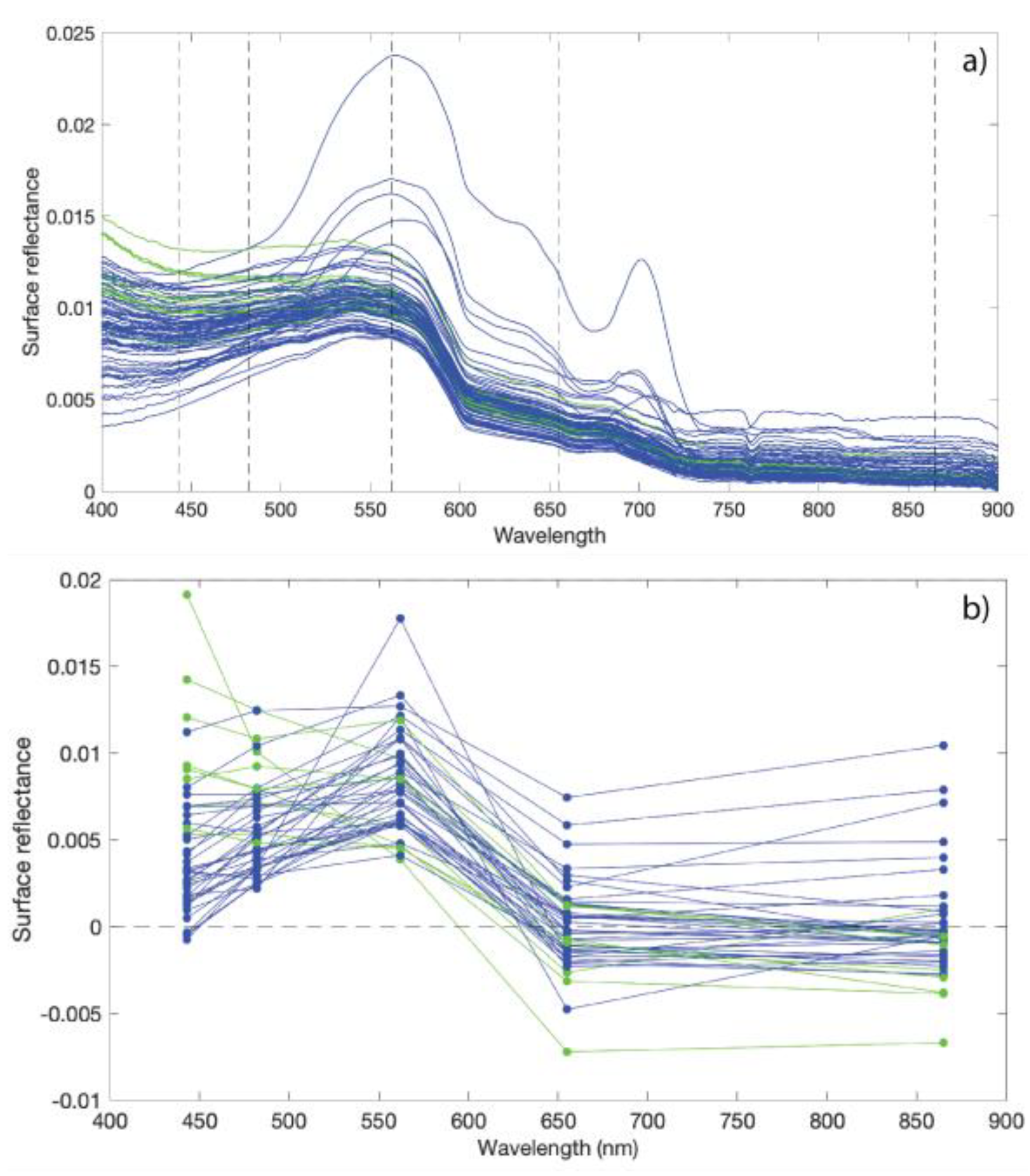
3.1. In Situ Surface Reflectance

An independent dataset of 85 in situ surface reflectance spectra were collected with an ASD spectroradiometer on 6 July 2023, 15 August 2023, 16 August 2023, and 8 September 2023. All spectra collected in the pelagic were of spectral shapes one and three (Figure 2a). Two spectra, collected near the shoreline where milfoil was visible from the surface, were of spectral shape two. Mats of the milfoil can become quite large and detach themselves from the substrate, collecting on structures such as the buoy and bridges. This could explain the presence of this spectral shape in the lake center. Spectral shape two pixels are also observed when wispy, light clouds are present over the lake (e.g., 26 September 2015, 24 October 2019). These observations led us to exclude pixels of spectral shape two from the analyses. In the in situ surface reflectance data, surface reflectance at Band 4 was never larger than at Band 2, so pixels with Band 4 greater than Band 2 were also removed from the analyses.

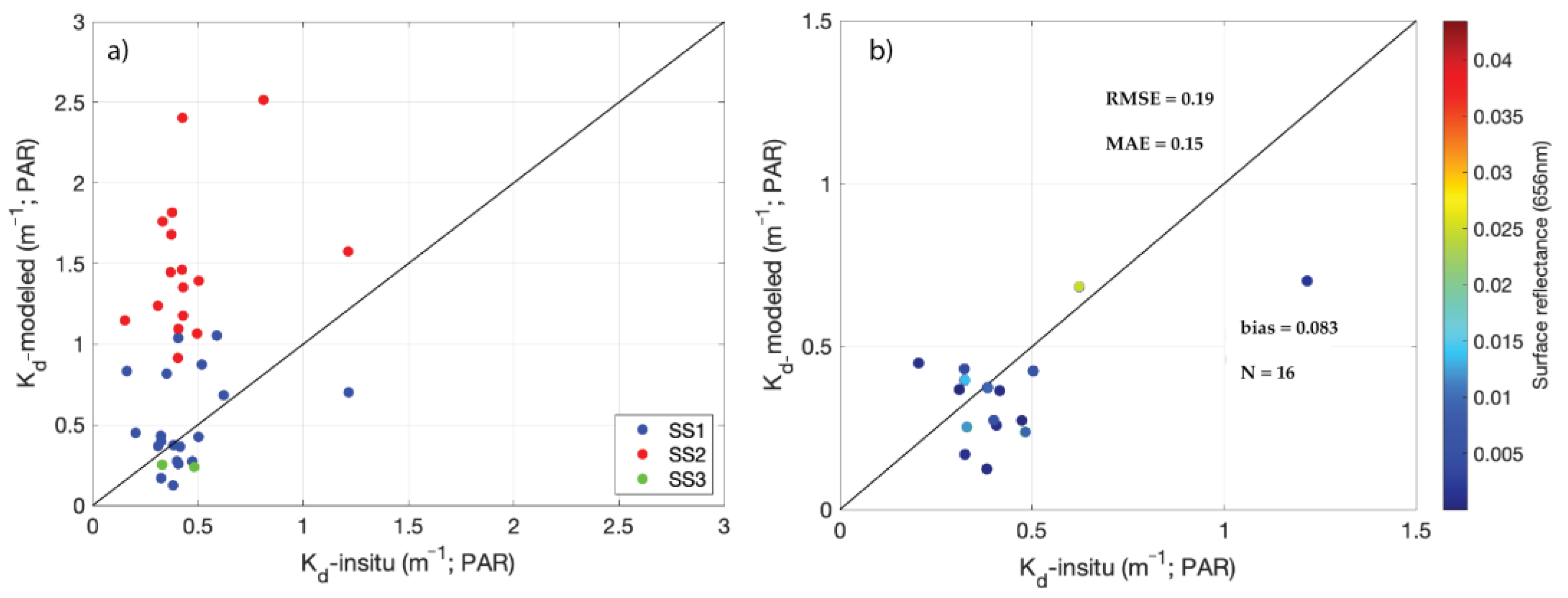
3.2. Performance of Semi-Analytical Models

3.2.1. QAA-v6 Lee-K_d(PAR)

Data collected from three sites (n = 16) containing concurrent measurements of K_d(PAR) and OLI surface reflectance were used to evaluate the performance of the IOP-based algorithm derived by [10]. We found that using the QAA-v6 for clear water (554 nm reference band) for calculation of the input IOPs yielded the K_d(PAR) values closest to the in-situ measurements. Previous research has also found that using a threshold value does not apply to inland lakes [59]. The RMSE, MAE, and bias were calculated as 0.19 m⁻¹, 0.15 m⁻¹, and 0.083 m⁻¹, respectively, and the model errors were not correlated with R_rs(656) (Figure 3b).

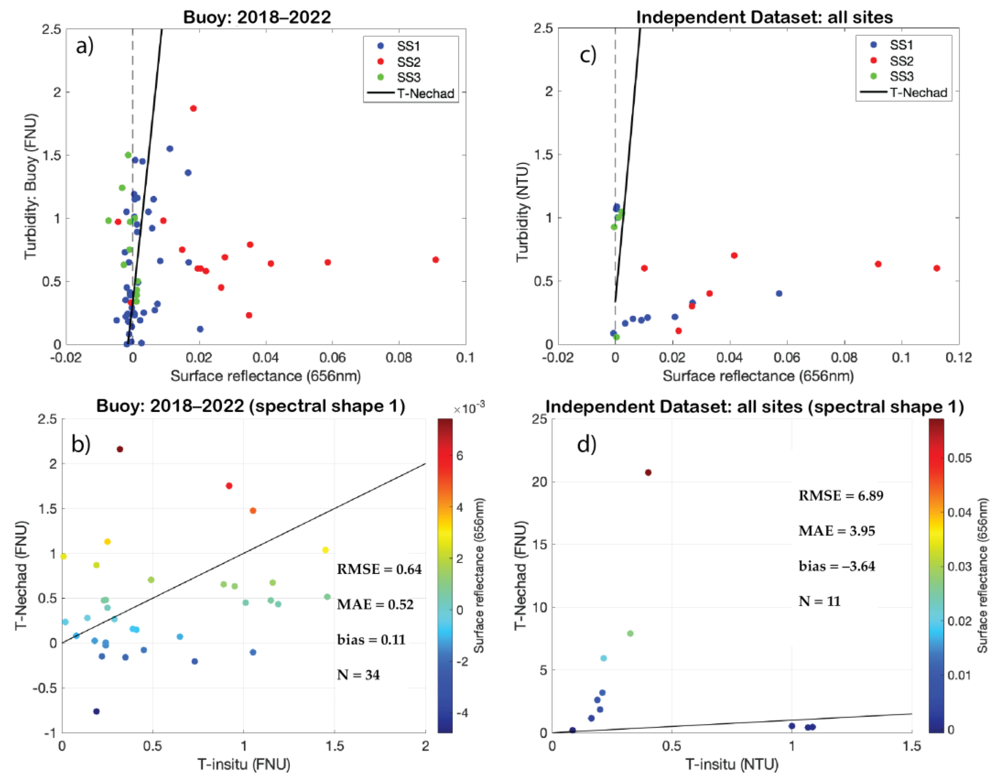
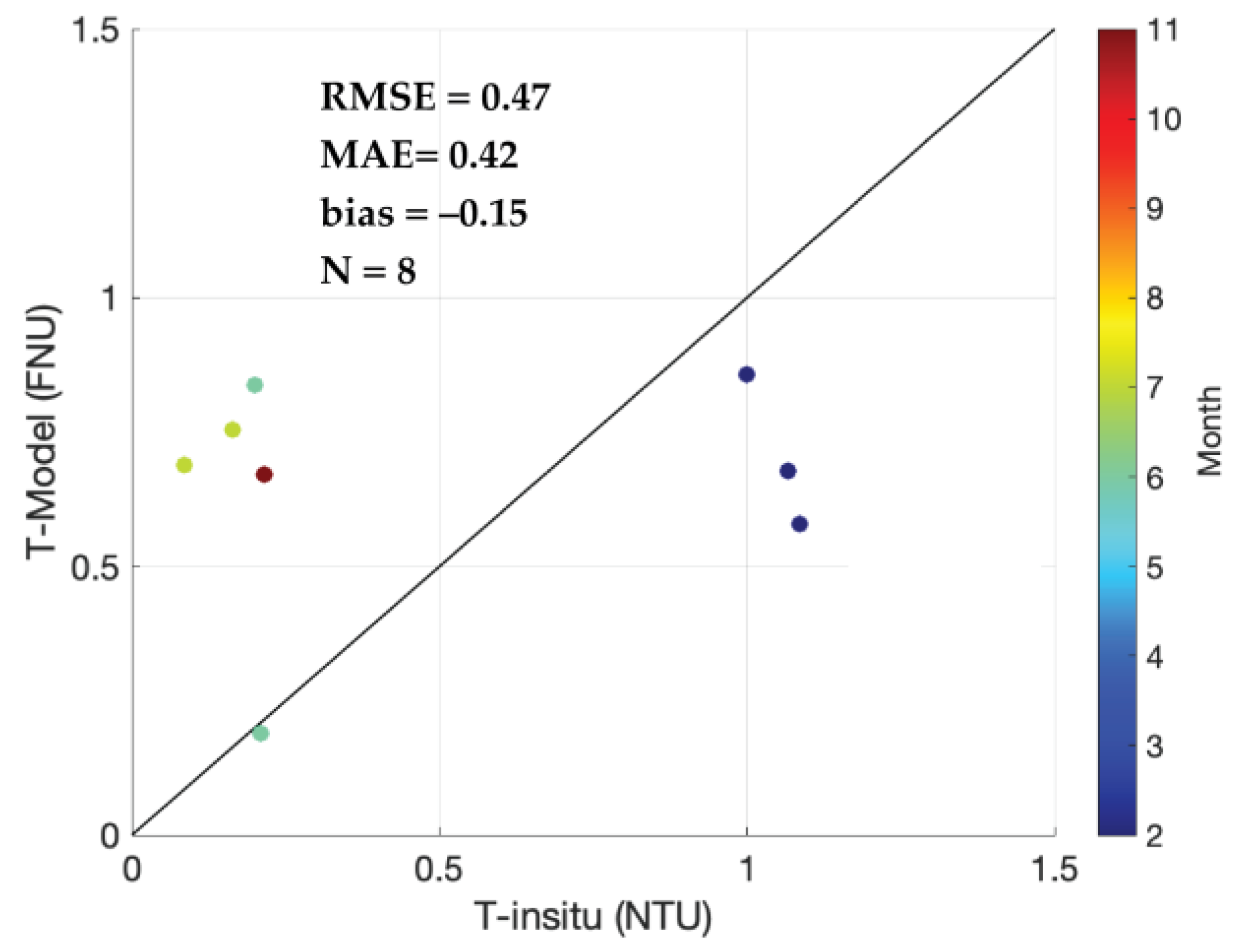
3.2.2. Nechad Turbidity

Data collected from the King County buoy (n = 34) and independently as part of this project (n = 11) containing concurrent measurements of turbidity and OLI ⍴_w(656) were used to evaluate the performance of the Nechad algorithm. For direct comparison to our regional model, model performance was evaluated both with and without spectral shape three pixels. When both spectral shapes one and three are included in the analysis at the buoy (n = 43), the RMSE, MAE, and bias were 0.78 FNU, 0.60 FNU, and 0.25 FNU, respectively. When spectral shape three was removed from the analysis (as for the regional turbidity algorithm), the model performance improved, and the RMSE, MAE, and bias decreased to 0.64, 0.51, and 0.11, respectively (Figure 4b). When both spectral shapes one and three are retained in the independent turbidity dataset (n = 16), the RMSE, MAE, and bias are equal to 5.7 FNU, 2.8 FNU, and −2.4, respectively. Unlike at the King County buoy, the model performance decreases when spectral shape three pixels are removed from the analysis (Figure 4d; RMSE = 6.9 FNU, MAE = 4.0 FNU, bias = −3.6 FNU).

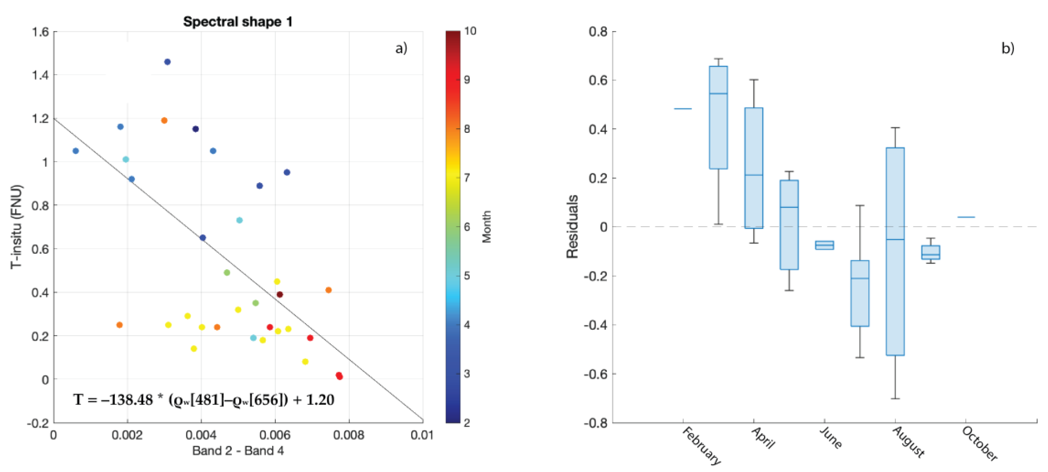
3.3. Regional Turbidity Algorithm

We derived a regional turbidity model based on spectral shape to improve turbidity predictions for Lake Washington. The difference between ⍴_w(481) and ⍴_w(656) had the highest correlation to in-situ turbidity for pixels with spectral shape one (Figure 5a;

Table 1. Correlation coefficients for spectral features used for deriving turbidity model. Spectral shape two (SS2) was identified as spectra resulting from the presence of visible macroalgae, so no turbidity model was derived for pixels with this spectral shape.

	B4-B1	B4-B2	B4-B3	B3-B2	B3-B1	B2-B1	Height B3
SS1	0.50	0.60	0.46	−0.026	0.072	0.20	−0.27
SS3	−0.080	−0.011	0.27	−0.25	−0.21	−0.15	−0.42

). We fit a least-squares linear model to these data:

$$Turbidity=intercept+slope\times \left({\rho }_w\left[481\right]-{\rho }_w\left[656\right]\right)$$

(10)

Coefficients and p-values for the model are presented in

Table 2. Turbidity model statistics.

Spectral Shape	RMSE	MAE	Bias	N *	p-Value
1	0.34	0.27	−3.4 × 10−16	34	0.00019
2	NA	NA	NA	15	NA
3	NA	NA	NA	9	NA

^* Counted after removal of spectral outliers for spectral shapes one and three (i.e., OLI Band 4 > Band 2).

. RMSE, MAE, and bias were calculated as 0.34 FNU, 0.27 FNU, and −3.4 × 10⁻¹⁶ FNU, respectively. No relationship between the model residuals and ⍴_w(656) was observed. The errors, on the other hand, were related to month, with the largest residuals observed in March and August. No statistically significant model could be derived for spectral shape three pixels, so these data were removed from the turbidity analysis.

We used the turbidity dataset collected independently as part of this project to evaluate the empirical models derived using the buoy dataset (described above). The RMSE, MAE, and bias were calculated as 0.47 NTU, 0.42 NTU, and −0.15 NTU, respectively, an improvement over the Nechad algorithm (Figure 6). No relationship between the model residuals and ⍴_w(656) was observed. There was also no error pattern between sites; the algorithm performed equally at all sites.

To better understand the limitations of our turbidity model, we compared seasonal patterns in turbidity calculated from monthly medians using the 2018–2022 in-situ dataset and modeled turbidity from 2013 to 2022. The model failed to capture the March peak and overestimated turbidity in the summer and autumn (Figure 7a,b). We also found that absolute differences between modeled and measured turbidity at the buoy were positively correlated with chlorophyll a-to-turbidity ratios (Chl:T) except for in March, when model errors were the greatest, and in September, when Chl:T was the greatest (R = 0.63; Figure 7c). The full turbidity dataset is presented in Figure 8.

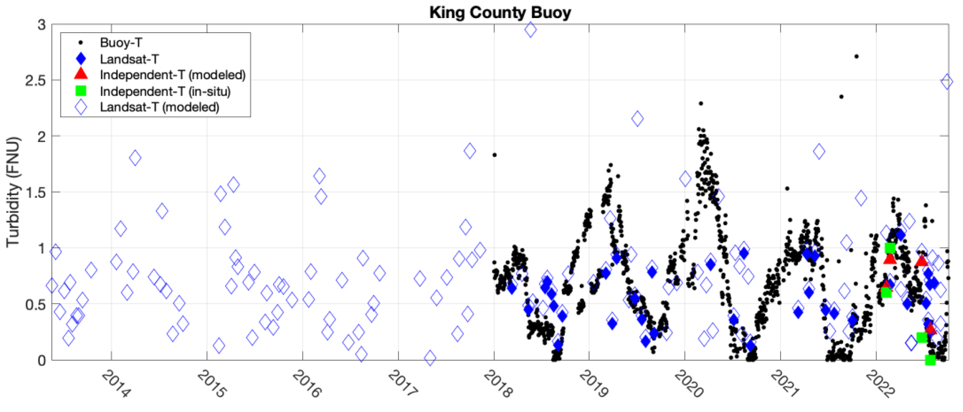
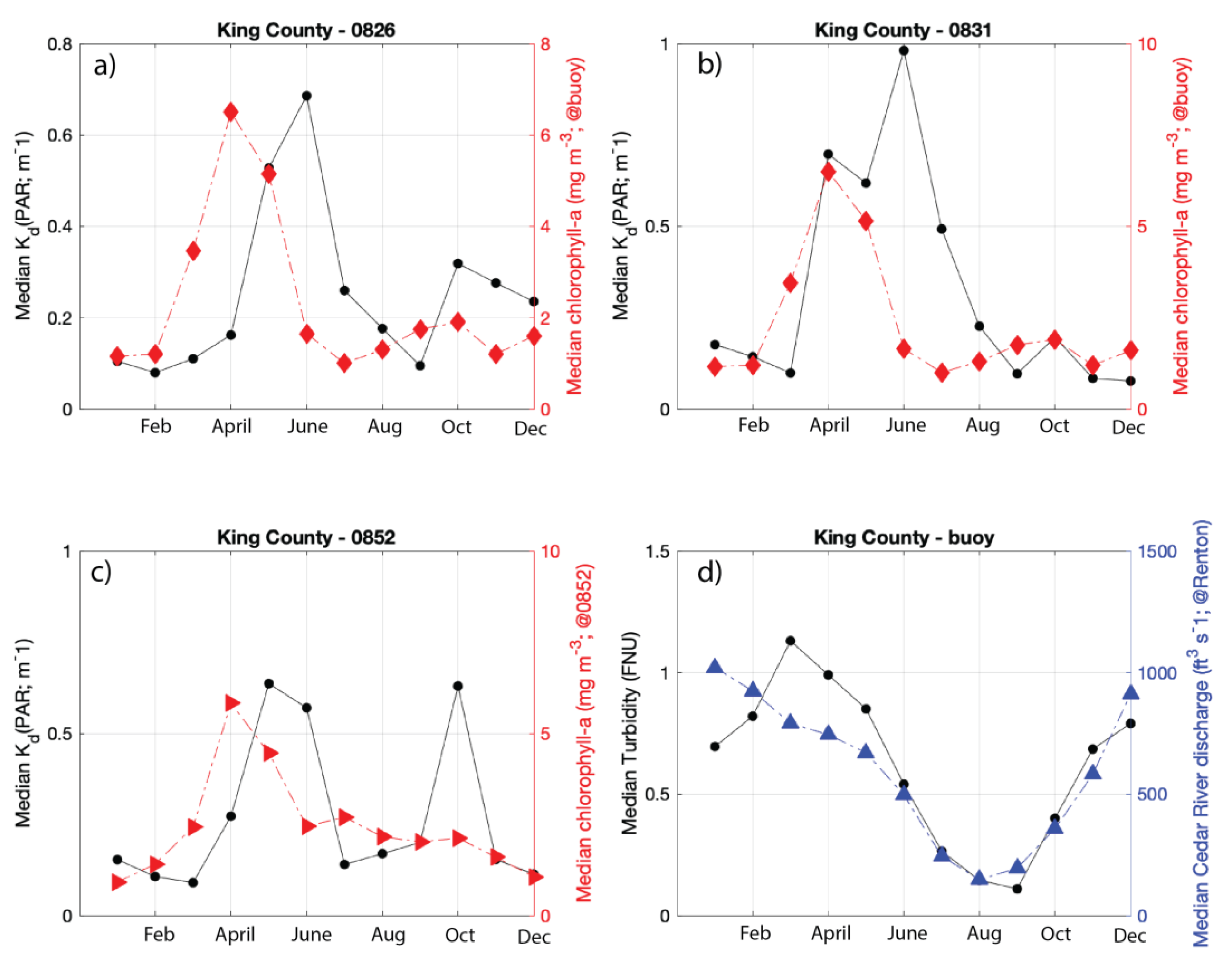
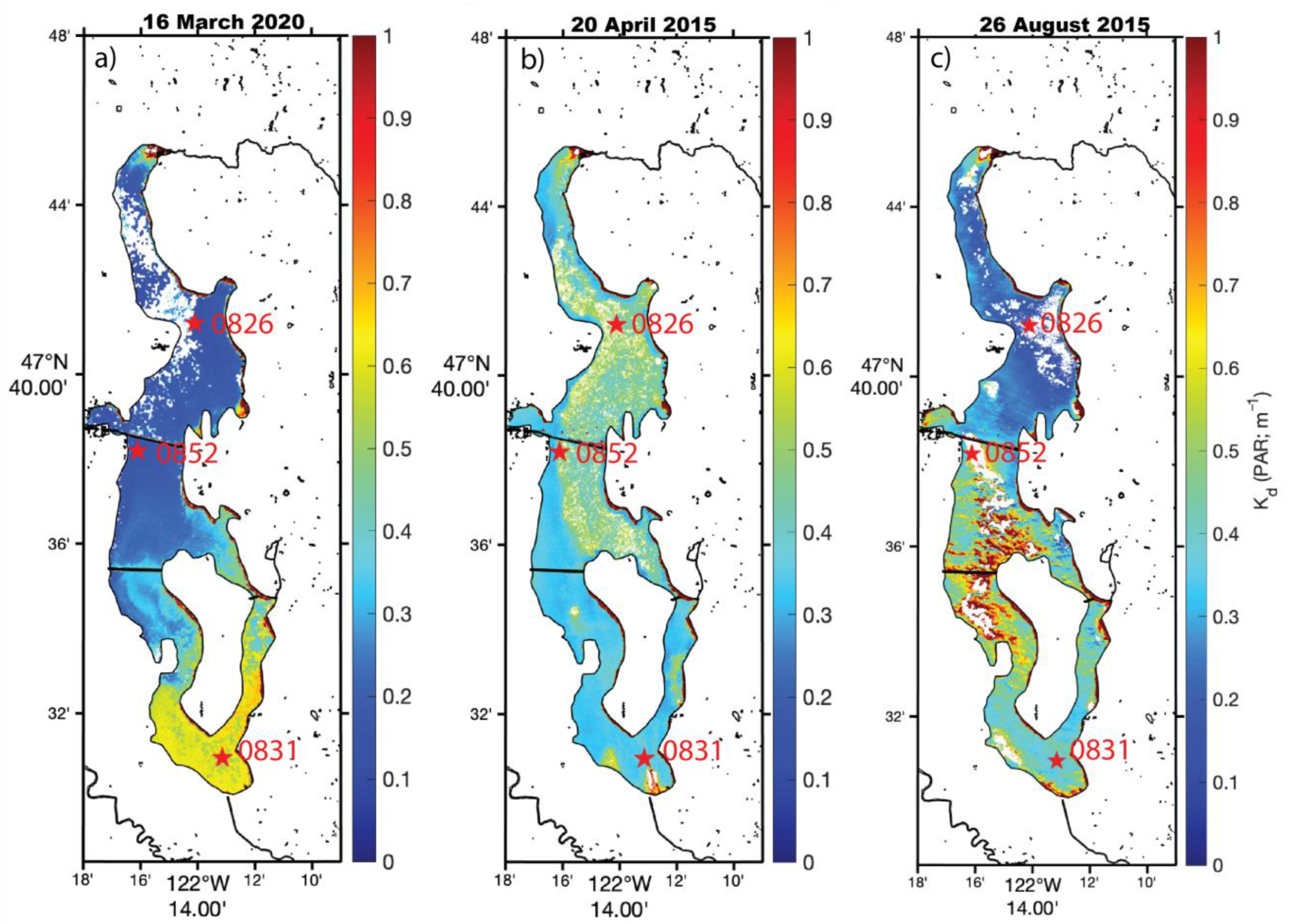
3.4. Spatiotemporal Water Clarity Variability

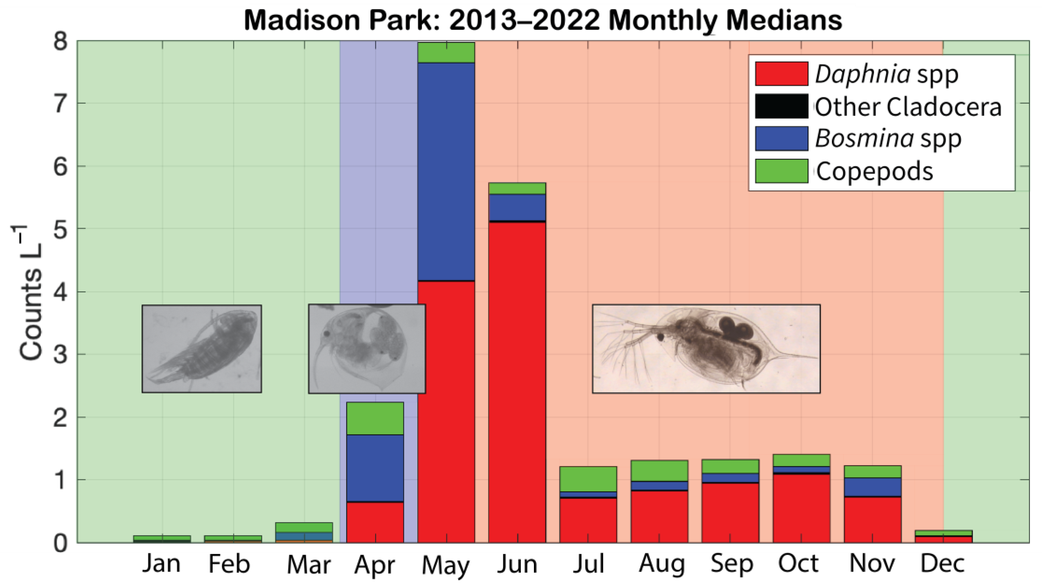
Landsat-8/9 OLI data were extracted from 2013 to 2022 at the four King County sites and used to evaluate annual and seasonal spatiotemporal variability in K_d(PAR) and turbidity. There were no significant trends at any of the King County sites in K_d(PAR) or turbidity (Mann–Kendall p > 0.05 for all sites) from 2013 to 2022 when the full and annual datasets were analyzed. Seasonal K_d(PAR) at the King County sites followed a similar pattern to each other; there exists a large spring peak at all sites (Figure 9a–c). At 0826 and 0852, elevated concentrations persist from May through June. The K_d(PAR) peaked at 0831, the site closest to the mouth of the Cedar River, begins in April and lasts through June. Additionally, K_d(PAR) peaks are present in the autumn (October) at all three sites. These autumn peaks, apparent in all K_d(PAR) datasets, are absent from the seasonal turbidity pattern, which nearly mirrors the seasonal variability in the Cedar River discharge rates over the same period (Figure 9d).

As for K_d(PAR), zooplankton abundances at Madison Park peaked in May through June, one month after the peak in chlorophyll a (Bosmina spp. peak in April with the onset of the spring bloom followed by high production of Daphnia in May–June) (Figure 10). In the autumn, zooplankton are most abundant in October, a pattern that becomes more pronounced when only the dominant group, Daphnia spp., is considered. No autumn chlorophyll a peak at 0852 (Madison Park) was present, though concentrations remain elevated through October. The chlorophyll a data collected from the buoy, however, indicate that phytoplankton concentrations in the autumn are the greatest in October. No time lag, thus, was present between autumn peaks of phytoplankton and zooplankton.

Example seasonal patterns showing the spatial variability in K_d(PAR) across the lake are presented in Figure 11. K_d(PAR) variability predominantly resulting from the Cedar River discharge is presented in Figure 11a, while biologically driven processes are driving K_d(PAR) variability in Figure 11b,c. Including a seasonal component to the model could potentially improve the model predictability by accounting for the seasonally different sources of variability (phytoplankton vs. fluvial) to the turbidity measurement.

4. Discussion

We used in-situ measurements to evaluate existing semi-analytical models for K_d(PAR) and turbidity, developed a regional turbidity model based on spectral shape, and evaluated the spatial and temporal trends in Lake Washington from 2013 to 2022. The MAE was 0.15 m⁻¹ for the QAA-v6 Lee K_d(PAR) algorithm, a 31% error (mean in-situ K_d(PAR) equal to 0.49 m⁻¹) for OLI pixels with spectral shapes one and three. This error is significant when K_d is used to model irradiance at depth. For example, at 10 m there is more than a fourfold difference in modeled irradiances given K_d equal to 0.49 m⁻¹ ± 0.15 m⁻¹. The differences between irradiances calculated at 20 m increases to twentyfold. Thus, for application to fisheries research in Lake Washington, which requires knowledge of the light field at the depths at which the fishes are found, the QAA-v6 Lee K_d(PAR) algorithm does not achieve the required accuracy.

The error observed in the QAA-v6 Lee K_d(PAR) algorithm, however, is within the range observed by [60], which utilized more than 1000 radiometric comparisons from both inland and coastal waters to examine the quality of derived aquatic reflectance values (⍴_w) from Landsat. For inland water observations, the median errors in ⍴_w(560) and ⍴_w(664) ranged from 20 to 30%, which yielded 25–70% uncertainties in derived chlorophyll a and total suspended solids (TSS) products. Additionally, the authors of [15] calculated a 93.9% mean absolute percent error when using the QAA-v6 Lee K_d(PAR) algorithm in a Chilean lake. Using the QAA-v5 algorithm, however, significantly increased model performance in their study and suggests a path forward to improve model predictability in Lake Washington.

Despite the uncertainty in the QAA-v6 K_d(PAR) product, a common seasonal pattern existed among all sites across the lake. At Madison Park (also King County site 0852), K_d(PAR) peaked in May through June, coincident with the peak in total zooplankton abundances. Further, Daphnia spp., which are particularly effective phytoplankton grazers compared to other zooplankton and have been found to improve transparency in Lake Washington [61], are most abundant in June, which is coincident with the significant decrease in chlorophyll a. This implies that zooplankton production was stimulated by the spring phytoplankton bloom, but the zooplankton were not capable of grazing down the phytoplankton to increase transparency until June, when Daphnia spp. become the dominant members of the zooplankton community. The autumn K_d(PAR) peak was observed in October at all sites, which is also coincident with maximum autumn zooplankton concentrations. This lends confidence to our results and suggests that the variability in K_d(PAR) is driven by biological processes (i.e., phytoplankton and zooplankton production).

We also used in-situ measurements and Landsat OLI data to develop a regional model for deriving turbidity concentrations that performed within the expected range of error (83% mean absolute error). Model errors increased as the relative proportion of chlorophyll a increased (R = 0.63), except in March and September, when the errors were decoupled from the chlorophyll a-to-turbidity ratio. Changes in particle type from seasonal phytoplankton succession and model uncertainty are likely, at least partially, responsible for the observed error.

Beginning in the summer and lasting through autumn, a shift in phytoplankton community structure has previously been observed. The authors of [22] observed a significant change in the phytoplankton community structure with the onset of summer (and stratified conditions), characterized by a shift from predominantly diatoms to chlorophytes and cyanophytes. Cryptophytes also increased in relative proportion. This shift in phytoplankton groups was accompanied by a shift in bulk pigments, which impacts the surface reflectance spectral shape. The primary pigments characteristic of diatoms are chlorophyll c₂ and fucoxanthin, which have absorption peaks at (in vivo) 450 nm and (in acetone) 468.3 nm, respectively [62]. Chlorophytes, on the other hand, are characterized by the presence of chlorophyll b and lutein, which have characteristic absorption peaks at (in vivo) 480 nm and (in acetone) 476.3 nm, respectively. Cyanophytes and cryptophytes are characterized by the pigments zeaxanthin and alloxanthin, respectively, which have absorption peaks at 480.9 nm and 483.5 nm [62]. Overall, this suggests that the absorption of light at OLI Band 2 (481 nm) could potentially be greater in the summer/autumn, which would result in reduced surface reflectance (⍴_w~R_rs~b_b/a+b_b). This reduction in ⍴_w(481) would result in a smaller than predicted difference between Band 2 and Band 4 (predictor variable) for a given turbidity concentration, assuming that most of the variability is being driven by changes in Band 2 (chlorophyll b has the second, smaller absorption peak at Band 4, for example, so this assumption is not strictly true). Alternatively, when diatoms dominate the phytoplankton community, a larger than predicted difference between Bands 4 and 2 would be observed (with a shift to a greater proportion of chlorophyll c₂ and fucoxanthin). In addition, since the difference between Bands 2 and 4 and turbidity are inversely related (Figure 5a), this would lead to an underestimation of in-situ turbidity in the spring and an overestimation in the summer/autumn.

This hypothesis is consistent with our observations that modeled turbidity was underestimated in the spring when chlorophyll a concentrations peaked (and diatoms dominated the phytoplankton community) and overestimated in the summer/autumn when chlorophyll a concentrations were also elevated (and chlorophytes, cyanophytes, and cryptophytes became more abundant) (Figure 7a). This further emphasizes how incorporating seasonality into the turbidity model would likely improve model performance. This was attempted as part of this research, but there were not enough satellite–in-situ matchups for the derivation of a seasonally-dependent model.

Turbidity at the buoy peaks in March, two months before K_d(PAR) peaks at 0852 and one month before chlorophyll a concentrations become elevated. Further, no autumn increase in turbidity is observed. These results suggest that the turbidity measurement is more sensitive to changes in water clarity associated with river flow, while the K_d(PAR) measurement is more sensitive to changes in biological processes (i.e., phytoplankton production and zooplankton abundance).

Accurate measurements or estimates of different optical properties of a water body are critical for understanding biotic processes such as the foraging behaviors of both planktivores and piscivores in aquatic ecosystems. Estimates of K_d and surface light enable estimates of how light at depth affects the reaction distance of a predator to prey fishes. In addition to how turbidity affects light at depth, the backscattering between predators and prey reduces the reaction distance exponentially as turbidity increases above 1.5 FNU, given the ambient light at depth [5,32]. Thus, mapping regional and depth-specific light and turbidity becomes the necessary first step toward mapping the spatiotemporal dynamics of predation risk or foraging success across a water body or watershed. These applications could become powerful tools for identifying and prioritizing restoration efforts that effectively target predation or feeding bottlenecks caused by habitat anomalies or human perturbations that affect underwater light or turbidity in ways that reduce survival or growth of valuable aquatic species.

In our study, we primarily focused on using two of the observed spectral shapes in the OLI dataset to calculate turbidity and K_d(PAR). However, we observed the third spectral shape that could not be directly evaluated for water clarity. This spectral shape, identified as spectral shape two, was observed only twice (out of 85 total spectra) using the ASD spectroradiometer where milfoil was clearly visible from the lake surface near the shoreline. Eurasian milfoil significantly alters the aquatic environment. It often forms dense canopies at the water surface that significantly reduce water clarity and light penetration. Additionally, the milfoil causes changes in water chemistry that can lead to significant variations in the dissolved oxygen concentration [40,63], thus making the habitat unsuitable for salmonids and other fishes. The distribution of Northern Pikeminnow (Ptychocheilus oregonensis), a sockeye predator, shifts further offshore beyond dense nearshore stands of Eurasian milfoil, further increasing predation on and reducing the success of juvenile sockeye [64].

Across Washington, the presence of Eurasian milfoil has been documented in nearly 150 lakes and major rivers [38]. Historically, various management approaches have been employed to control the spread of this invasive plant, including chemical treatments, mechanical removal, and manual control efforts such as diver-assisted suction harvesting (DASH) and harvesting machines [65]. Our findings have the potential to significantly contribute to these ongoing management efforts by offering valuable insights into the large-scale spatial and temporal distributions of Eurasian milfoil. This comprehensive understanding of milfoil dynamics could help to inform and refine the strategies employed for its control and mitigation across the affected lakes and rivers in Washington and globally.

5. Conclusions

In this study, we evaluated the QAA-v6 Lee K_d(PAR) algorithm and developed a regional turbidity algorithm using coincident in-situ measurements and Landsat-8/9 OLI surface reflectance data at multiple sites in Lake Washington. These algorithms were applied to a decade-long dataset spanning from 2013 to 2022 to investigate spatiotemporal patterns in water clarity. No trend in K_d(PAR) or turbidity was observed at any of the King County sites when the annually averaged and full datasets were considered.

Our research identified distinct sensitivities between the K_d(PAR) measurement to biological variability and the turbidity measurement to changes in water clarity linked to river flow. These insights have implications for future monitoring and management efforts, as they highlight the need for tailored approaches when addressing water quality challenges associated with these distinct sources of variability.

Looking ahead, our ongoing data collection efforts, combined with information on nighttime light distributions and fish behaviors, will play a crucial role in understanding the mechanisms contributing to regional declines in juvenile salmon populations due to predation by visually feeding predators in the Lake Washington basin. This research not only advances our understanding of the dynamics of this unique ecosystem but also contributes to broader discussions surrounding the conservation and sustainability of freshwater resources in the face of evolving environmental pressures.

References

1. ISO 7027-1:2016; Water quality-determination of turbidity. ISO: Geneva, Switzerland, 2016.
2. Davies-Colley, R.J.; Smith, D.G. Turbidity, suspended sediment, and water clarity: A review. J. Am. Water Resour. Assoc. 2001, 37, 1085–1101. [Google Scholar] [CrossRef]
3. Turner, J.S.; Fall, K.A.; Friedrichs, C.T. Clarifying water clarity: A call to use metrics best suited to corresponding research and management goals in aquatic ecosystems. Limnol. Oceanogr. Lett. 2022, 8, 388–397. [Google Scholar] [CrossRef]
4. Levy, D.A. Sensory mechanism and selective advantage for diel vertical migration in juvenile sockeye salmon, Oncorhynchus nerka. Can. J. Fish. Aquat. Sci. 1990, 47, 1796–1802. [Google Scholar] [CrossRef]
5. Beauchamp, D.A.; Baldwin, C.M.; Vogel, J.L.; Gubala, C.P. Estimating diel, depth-specific foraging with a visual encounter rate model for pelagic piscivores. Can. J. Fish. Aquat. Sci. 1999, 56 (Suppl. S1), 128–139. [Google Scholar] [CrossRef]
6. Bunnell, D.B.; Ludsin, S.A.; Knight, R.L.; Rudstam, L.G.; Williamson, C.E.; Höök, T.O.; Collingsworth, P.D.; Lesht, B.M.; Barbiero, R.P.; Scofield, A.E.; et al. Consequences of changing water clarity on the fish and fisheries of the Laurentian Great Lakes. Can. J. Fish. Aquat. Sci. 2021, 78, 1524–1542. [Google Scholar] [CrossRef]
7. Jamet, C.; Loisel, H.; Dessailly, D. Retrieval of the spectral diffuse attenuation coefficient Kd(λ) in open and coastal ocean waters using a neural network inversion: Retrieval of Diffuse Attenuation. J. Geophys. Res. Ocean. 2012, 117, C10023. [Google Scholar] [CrossRef]
8. Begouen Demeaux, C.; Boss, E. Validation of Remote-Sensing Algorithms for Diffuse Attenuation of Downward Irradiance Using BGC-Argo Floats. Remote Sens. 2022, 14, 4500. [Google Scholar] [CrossRef]
9. Rubin, H.J.; Lutz, D.A.; Steele, B.G.; Cottingham, K.L.; Weathers, K.C.; Ducey, M.J.; Palace, M.; Johnson, K.M.; Chipman, J.W. Remote Sensing of Lake Water Clarity: Performance and Transferability of Both Historical Algorithms and Machine Learning. Remote Sens. 2021, 13, 1434. [Google Scholar] [CrossRef]
10. Lee, Z.; Du, K.; Arnone, R.; Liew, S.; Penta, B. Penetration of solar radiation in the upper ocean: A numerical model for oceanic and coastal waters. J. Geophys. Res. Ocean. 2005, 110, C09019. [Google Scholar] [CrossRef]
11. Lee, Z.; Hu, C.; Shang, S.; Du, K.; Lewis, M.; Arnone, R.; Brewin, R. Penetration of UV-visible solar radiation in the global oceans: Insights from ocean color remote sensing. J. Geophys. Res. Ocean. 2013, 118, 4241–4255. [Google Scholar] [CrossRef]
12. Lee, Z.; Carder, K.L.; Arnone, R.A. Deriving inherent optical properties from water color: A multiband quasi-analytical algorithm for optically deep waters. Appl. Opt. 2002, 41, 5755–5772. [Google Scholar] [CrossRef] [PubMed]
13. Lee, Z.; Shang, S.; Qi, L.; Yan, J.; Lin, G. A semi-analytical scheme to estimate Secchi-disk depth from Landsat-8 measurements. Remote Sens. Environ. 2016, 177, 101–106. [Google Scholar] [CrossRef]
14. Yin, Z.; Li, J.; Liu, Y.; Xie, Y.; Zhang, F.; Wang, S.; Sun, X.; Zhang, B. Water clarity changes in Lake Taihu over 36 years based on Landsat TM and OLI observations. Int. J. Appl. Earth Obs. Geoinf. 2021, 102, 102457. [Google Scholar] [CrossRef]
15. Rodríguez-López, L.; González-Rodríguez, L.; Duran-Llacer, I.; García, W.; Cardenas, R.; Urrutia, R. Assessment of the diffuse attenuation coefficient of photosynthetically active radiation in a Chilean Lake. Remote Sens. 2022, 14, 4568. [Google Scholar] [CrossRef]
16. Keith, D.J.; Salls, W.; Schaeffer, B.A.; Werdell, P.J. Assessing the suitability of lakes and reservoirs for recreation using Landsat 8 Water Clarity. Res. Sq. 2023. [Google Scholar] [CrossRef]
17. Nechad, B.; Ruddick, K.G.; Neukermans, G. September. Calibration and validation of a generic multisensor algorithm for mapping of turbidity in coastal waters. In Remote Sensing of the Ocean, Sea Ice, and Large Water Regions 2009; SPIE: Bellingham, WA, USA, 2009; Volume 7473, pp. 161–171. [Google Scholar]
18. Dogliotti, A.I.; Ruddick, K.G.; Nechad, B.; Doxaran, D.; Knaeps, E. A single algorithm to retrieve turbidity from remotely-sensed data in all coastal and estuarine waters. Remote Sens. Environ. 2015, 156, 157–168. [Google Scholar] [CrossRef]
19. Potes, M.; Costa, M.J.; Salgado, R. Satellite remote sensing of water turbidity in Alqueva reservoir and implications on lake modelling. Hydrol. Earth Syst. Sci. 2012, 16, 1623–1633. [Google Scholar] [CrossRef]
20. Hossain, A.A.; Mathias, C.; Blanton, R. Remote sensing of turbidity in the Tennessee River using Landsat 8 satellite. Remote Sens. 2021, 13, 3785. [Google Scholar] [CrossRef]
21. Edmondson, W.T. Sixty years of Lake Washington: A curriculum vitae. Lake Reserv. Manag. 1994, 10, 75–84. [Google Scholar] [CrossRef]
22. Arhonditsis, G.; Brett, M.T.; Frodge, J. Environmental control and limnological impacts of a large recurrent spring bloom in Lake Washington, USA. Environ. Manag. 2003, 31, 0603–0618. [Google Scholar] [CrossRef]
23. Fresh, K.L. Lake Washington fish: A historical perspective. Lake Reserv. Manag. 1994, 9, 148–151. [Google Scholar] [CrossRef]
24. Kendall, N.W.; Quinn, T.P.; Beauchamp, D.A.; Fresh, K.; Volk, C.; Unrein, J. Life-cycle model reveals sensitive life stages and evaluates recovery options for a dwindling Pacific salmon population. N. Am. J. Fish. Manag. 2022, 43, 203–230. [Google Scholar] [CrossRef]
25. Vogel, J.L.; Beauchamp, D.A. Effects of light, prey size, and turbidity on reaction distances of lake trout (Salvelinus namaycush) to salmonid prey. Can. J. Fish. Aquat. Sci. 1999, 56, 1293–1297. [Google Scholar] [CrossRef]
26. Mazur, M.M.; Beauchamp, D.A. A comparison of visual prey detection among species of piscivorous salmonids: Effects of light and low turbidities. Environ. Biol. Fishes 2003, 67, 397–405. [Google Scholar] [CrossRef]
27. Utne-Palm, A.C. Visual feeding of fish in a turbid environment: Physical and behavioral aspects. Mar. Freshw. Behav. Physiol. 2002, 35, 111–128. [Google Scholar] [CrossRef]
28. Fiksen, Ø.; Aksnes, D.L.; Flyum, M.H.; Giske, J. The influence of turbidity on growth and survival of fish larvae: A numerical analysis. In Proceedings of the Sustainable Increase of Marine Harvesting: Fundamental Mechanisms and New Concepts: Proceedings of the 1st Maricult Conference held in Trondheim, Norway, 25–28 June 2000; Springer: Dordrecht, The Netherlands, 2002; pp. 49–59. [Google Scholar]
29. Hansen, A.G.; Beauchamp, D.A.; Schoen, E.R. Visual prey detection responses of piscivorous trout and salmon: Effects of light, turbidity, and prey size. Trans. Am. Fish. Soc. 2013, 142, 854–867. [Google Scholar] [CrossRef]
30. Beauchamp, D.A.; Stewart, D.J.; Thomas, G.L. Corroboration of a bioenergetics model for sockeye salmon. Trans. Am. Fish. Soc. 1989, 118, 597–607. [Google Scholar] [CrossRef]
31. Hovel, R.A.; Thorson, J.T.; Carter, J.L.; Quinn, T.P. Within-lake habitat heterogeneity mediates community response to warming trends. Ecology 2017, 98, 2333–2342. [Google Scholar] [CrossRef] [PubMed]
32. Hansen, A.G.; Beauchamp, D.A. Effects of prey abundance, distribution, visual contrast and morphology on selection by a pelagic piscivore. Freshw. Biol. 2014, 59, 2328–2341. [Google Scholar] [CrossRef]
33. Thomas, Z.R.; Beauchamp, D.A.; Clark, C.P.; Quinn, T.P. Seasonal shifts in diel vertical migrations by lake-dwelling coastal cutthroat trout, Oncorhynchus clarkii clarkii, reflect thermal regimes and prey distributions. Ecol. Freshw. Fish 2023, 32, 842–851. [Google Scholar] [CrossRef]
34. Kitano, J.; Mori, S.; Peichel, C.L. Divergence of male courtship displays between sympatric forms of anadromous threespine stickleback. Behaviour 2008, 145, 443–461. [Google Scholar]
35. Quinn, T.P.; Sergeant, C.J.; Beaudreau, A.H.; Beauchamp, D.A. Spatial and temporal patterns of vertical distribution for three planktivorous fishes in Lake Washington. Ecol. Freshw. Fish 2012, 21, 337–348. [Google Scholar] [CrossRef]
36. Hansen, A.G.; Beauchamp, D.A. Latitudinal and photic effects on diel foraging and predation risk in freshwater pelagic ecosystems. J. Anim. Ecol. 2015, 84, 532–544. [Google Scholar] [CrossRef]
37. Patmont, C.R.; Davis, J.I.; Swartz, R.G. Aquatic Plants in Selected Waters of King County: Distribution and Community Composition of Macrophytes; Municipality of Metropolitan Seattle, Water Quality Division: Seattle, WA, USA, 1981. [Google Scholar]
38. Olden, J.D.; Tamayo, M. Incentivizing the public to support invasive species management: Eurasian milfoil reduces lakefront property values. PLoS ONE 2014, 9, e110458. [Google Scholar] [CrossRef]
39. Parsons, J.K.; Marx, G.E.; Divens, M. A study of Eurasian watermilfoil, macroinvertebrates and fish in a Washington lake. J. Aquat. Plant Manag. 2011, 49, 71–82. [Google Scholar]
40. Frodge, J.D.; Thomas, G.L.; Pauley, G.B. Effects of canopy formation by floating and submergent aquatic macrophytes on the water quality of two shallow Pacific Northwest lakes. Aquat. Bot. 1990, 38, 231–248. [Google Scholar] [CrossRef]
41. Frodge, J.D.; Marino, D.A.; Pauley, G.B.; Thomas, G.L. Mortality of largemouth bass (Micropterus salmoides) and steelhead trout (Oncorhynchus mykiss) in densely vegetated littoral areas tested using in situ bioassay. Lake Reserv. Manag. 1995, 11, 343–358. [Google Scholar] [CrossRef]
42. Sound, I.P. Recommended Guidelines for Sampling Marine Sediment, Water Column, and Tissue; Puget Sound Water Quality Action Team: Olympia, WA, USA, 1997. [Google Scholar]
43. King County Environmental Laboratory (KCEL). Standard Operating Procedure for SBE 25 Plus SeaLogger CTD. SOP # 220v5; KCEL, Water and Land Resources Division: Seattle, WA, USA, 2017. [Google Scholar]
44. Zaneveld, J.R.V.; Barnard, A.H.; Boss, E. Theoretical derivation of the depth average of remotely sensed optical parameters. Opt. Express 2005, 13, 9052–9061. [Google Scholar] [CrossRef] [PubMed]
45. King County: Lakes. Available online: https://green2.kingcounty.gov/lake-buoy/Data.aspx. (accessed on 10 October 2022).
46. YSI Turbidity Sensors. Available online: https://www.ysi.com/filelibrary/documents/technicalnotes/t627_turbidity_units_and_calibration_solutions.pdf. (accessed on 1 September 2023).
47. Mueller, J.L.; Pietras, C.; Hooker, S.B.; Austin, R.W.; Miller, M.; Knobelspiesse, K.D.; Frouin, R.; Holben, B.; Voss, K. Ocean Optics Protocols for Satellite Ocean Color Sensor Validation, Revision 5. Volume V: Biogeochemical and Bio-Optical Measurements and Data Analysis Protocols; Goddard Space Flight Space Center: Greenbelt, MD, USA, 2003; pp. 1–43, (NASA/TM-2003-). [Google Scholar] [CrossRef]
48. Zhang, Y.; Liu, M.L.; Qin, B.; van der Woerd, H.J.; Li, J.; Li, Y. Modeling Remote-Sensing Reflectance and Retrieving Chlorphyll-a Concentration in Extremely Turbid Case-2 Waters (Lake Taihu, China). IEEE Trans. Geosci. Remote Sens. 2009, 47, 1937–1948. [Google Scholar] [CrossRef]
49. EarthExplorer. Available online: earthexplorer.usgs.gov. (accessed on 12 July 2022).
50. Landsat Collection-2 Level-2 Science Products. Available online: https://www.usgs.gov/landsat-missions/landsat-collection-2-level-2-science-products. (accessed on 12 July 2022).
51. Franz, B.A.; Bailey, S.W.; Kuring, N.; Werdell, P.J. Ocean color measurements with the Operational Land Imager on Landsat-8: Implementation and evaluation in SeaDAS. J. Appl. Remote Sens. 2015, 9, 096070. [Google Scholar] [CrossRef]
52. Vanhellemont, Q.; Ruddick, K. Advantages of high quality SWIR bands for ocean colour processing: Examples from Landsat-8. Remote Sens. Environ. 2015, 161, 89–106. [Google Scholar] [CrossRef]
53. King County Environmental Laboratory (KCEL). Standard Operating Procedure for Attended YSI EXO Multiprobe Operations. SOP#:245v1; King County Environmental Laboratory: Seattle, WA, USA, 2018. [Google Scholar]
54. National Water Information System USGS 12119000 Cedar River at Renton, WA. Available online: https://waterdata.usgs.gov/nwis/dv?referred_module=sw&site_no=12119000 (accessed on 14 April 2023).
55. Bogorov, V.G. To the methods of the zooplankton processing. Russ. Hydrobiol. J. 1927, 6, 193–198. [Google Scholar]
56. Update of the Quasi-Analytical Algorithm (QAA-v6). Available online: https://www.ioccg.org/groups/Software_OCA/QAA_v6_2014209.pdf. (accessed on 8 March 2023).
57. Nechad, B.; Ruddick, K.G.; Park, Y. Calibration and validation of a generic multisensor algorithm for mapping of total suspended matter in turbid waters. Remote Sens. Environ. 2010, 114, 854–866. [Google Scholar] [CrossRef]
58. Fatichi, S. Mann-Kendall Modified Test. MATLAB Central File Exchange. Available online: https://www.mathworks.com/matlabcentral/fileexchange/25533-mann-kendall-modified-test (accessed on 10 August 2023).
59. Chen, M.; Xiao, F.; Wang, Z.; Feng, Q.; Ban, X.; Zhou, Y.; Hu, Z. An Improved QAA-Based Method for Monitoring Water Clarity of Honghu Lake Using Landsat TM, ETM+ and OLI Data. Remote Sens. 2022, 14, 3798. [Google Scholar] [CrossRef]
60. Pahlevan, N.; Mangin, A.; Balasubramanian, S.V.; Smith, B.; Alikas, K.; Arai, K.; Barbosa, C.; Bélanger, S.; Binding, C.; Bresciani, M.; et al. ACIX-Aqua: A global assessment of atmospheric correction methods for Landsat-8 and Sentinel-2 over lakes, rivers, and coastal waters. Remote Sens. Environ. 2021, 258, 112366. [Google Scholar] [CrossRef]
61. Edmondson, W.T.; Litt, A.H. Daphnia in lake Washington 1. Limnol. Oceanogr. 1982, 27, 272–293. [Google Scholar] [CrossRef]
62. Phytoplankton Pigments in Oceanography: Guidelines to Modern Methods; Wright, S.W.; Jeffrey, S.W.; Mantoura, R.F.C. (Eds.) Unesco Pub.: Paris, France, 2005. [Google Scholar]
63. Courtemanche, B.; Levac, E. Low-cost profiling buoys to assess the effect of Eurasian watermilfoil density on dissolved oxygen in the water column. In Proceedings of the AGU Fall Meeting 2022, Chicago, IL, USA, 12–16 December 2022; p. H22W-1149. [Google Scholar]
64. COSEWIC. COSEWIC Assessment and Status Report on the Sockeye Salmon Oncorhynchus nerka (Cultus Population) in Canada; Committee on the Status of Endangered Wildlife in Canada: Ottawa, ON, Canada, 2003. [Google Scholar]
65. Codd-Downey, R.; Jenkin, M.; Dey, B.B.; Zacher, J.; Blainey, E.; Andrews, P. Monitoring re-growth of invasive plants using an autonomous surface vessel. Front Robot AI 2021, 7, 583416. [Google Scholar] [CrossRef]
Figure 1. (a) Map of Pacific Northwest with Lake Washington bounded in the red box. (b) Lake Washington’s 20 m, 40 m, and 60 m bathymetric contours mapped with the independent dataset (blue diamonds), King County (green triangles), and University of Washington (UW, Madison Park) sites. The King County buoy is indicated by the red star. Data are collected at the southern site and the buoy by both King County and as part of this research (independent dataset). King County and UW both collect data at Madison Park. The scale bar shows distance in miles. (c) Mapped Landsat-8 OLI spectral shapes corresponding to (d) collected on 20 April 2015. (d) Mean surface reflectance for three spectral shapes observed at the King County buoy.
Remotesensing 15 05055 g001
Figure 2. (a) Measurements of in-situ surface reflectance (unitless) from 400 to 900 nm. Spectral shape one spectra are shown in blue and spectral shape three spectra are shown in green. (b) OLI surface reflectance at the King County Buoy. Data shown in panels (a,b) are independent.
Remotesensing 15 05055 g002
Figure 3. (a) In-situ Kd(PAR) compared to QAA-v6 Lee Kd(PAR). The 1:1 relationship is indicated by the black line, and data are shown as a function of spectral shape classification. (b) In-situ Kd(PAR) compared to Kd(PAR) modeled for spectral shapes one and three. The 1:1 relationship is indicated by the black line, and data are shown as a function of surface reflectance at 656 nm.
Remotesensing 15 05055 g003
Figure 4. (a) Surface reflectance at 656 nm (⍴w(656)) plotted against in-situ turbidity at the King County buoy. Data are shown as a function of spectral shape. The Nechad model is shown by the black line and the dashed line is a vertical line drawn at 0. (b) In-situ turbidity compared to modeled turbidity at the buoy for spectral shape one. Data are plotted as a function of ⍴w(656). The black line shows the 1:1 relationship. (c) Where data were collected independently, surface reflectance ⍴w(656) plotted against in-situ turbidity with data shown as a function of spectral shape. The Nechad model shown in the black line and the dashed line is a vertical line drawn at 0. (d) In-situ turbidity compared to modeled turbidity at the independent sites for spectral shape one with data shown as a function of ⍴w(656).
Remotesensing 15 05055 g004
Figure 5. (a) Regional empirical turbidity model using OLI surface reflectance at 656 nm and 481 nm for deriving turbidity plotted as a function of month for spectral shape one. Spectral shape two was identified as pixels containing visible milfoil, so no model was derived for this spectral shape. No statistically significant model (⍺ = 0.05) could be derived using spectral shape three pixels. (b) Model residuals plotted as a function of month.
Remotesensing 15 05055 g005
Figure 6. In-situ (independent dataset) and modeled turbidity using the regional algorithm plotted as a function of month. The black line shows the 1:1 relationship.
Remotesensing 15 05055 g006
Figure 7. (a) Measured and modeled monthly median turbidity concentrations; (b) chlorophyll a-to-turbidity ratios (Chl:T; red dots) from the King County buoy plotted over absolute differences between measured and modeled turbidity; (c) absolute differences between measured and modeled turbidity related to buoy chlorophyll a-to-turbidity ratios with March and September turbidity values excluded. The dotted red line shows the linear fit.
Remotesensing 15 05055 g007
Figure 8. Turbidity at the buoy from 2013 to 2022. The buoy data are shown in the black dots. The in-situ and modeled turbidity data collected at the independent sites are shown in green squares and red triangles, respectively. The filled blue diamonds are the Landsat-8/9-based turbidity values that were used for model development, and the empty blue diamonds are the satellite-based turbidity values where no in-situ data were available.
Remotesensing 15 05055 g008
Figure 9. Monthly median chlorophyll a measurements, shown in red diamonds, collected at the buoy with monthly median Kd(PAR) values, shown in black circles, at (a) 0826 and (b) 0831; (c) monthly median chlorophyll a, shown in red triangles, and Kd(PAR) measurements, shown in black circles, at 0852; (d) monthly median Cedar River discharge rates at Renton, WA, shown in blue triangles, plotted with turbidity data collected at the King County buoy, shown in black circles.
Remotesensing 15 05055 g009
Figure 10. Median monthly zooplankton group (Daphnia spp., other Cladocera, Bosmina spp., copepods) abundances from 2013 to 2022 collected at Madison Park. A representative from each seasonally dominant group is pictured (Daphnia pulicaria (1.0–2.8 mm), Bosmina sp. (0.3–0.8 mm), Leptodiaptomus ashlandi (0.3–1.5 mm)).
Remotesensing 15 05055 g010
Figure 11. Spatial patterns in Kd(PAR) mapped for (a) 16 March 2020, when Kd(PAR) variability was primarily driven by the Cedar River; (b) 20 April 2015, when the spring phytoplankton bloom was the primary source of changing water clarity; (c) 26 August 2015, when the autumn bloom was driving the water clarity changes.
Remotesensing 15 05055 g011