Article

Spatiotemporal Heterogeneity of Water Conservation Function and Its Driving Factors in the Upper Yangtze River Basin

1
Key Laboratory of Water Cycle & Related Land Surface Processes, Institute of Geographic Sciences and Natural Resources Research, Chinese Academy of Sciences, Beijing 100101, China
2
University of Chinese Academy of Sciences, Beijing 100049, China
3
State Key Laboratory of Water Resources Engineering and Management, Wuhan University, Wuhan 430072, China
4
Guangdong Research Institute of Water Resources and Hydropower, Guangzhou 510635, China
*
Author to whom correspondence should be addressed.
Remote Sens. 2023, 15(21), 5246; https://doi.org/10.3390/rs15215246
Submission received: 15 August 2023 / Revised: 2 November 2023 / Accepted: 3 November 2023 / Published: 5 November 2023
(This article belongs to the Special Issue Advances in Remote Sensing of Ecohydrology)

Abstract

:
The water conservation function (WCF), as one of the most critical ecosystem services, has an important impact on the ecological sustainability of a region. Accurately characterizing the spatiotemporal heterogeneity of WCF and further exploring its driving factors are of great significance for river basin management. Here, the WCF of the upper Yangtze River basin (UYRB) from 1991 to 2020 was calculated using the water yield module in the Integrated Valuation of Ecosystem Service and Tradeoffs (InVEST) model. Also, we innovatively applied emerging hot spot analysis (EHSA), which could describe the location and pattern of historical changes more accurately, to investigate the spatiotemporal heterogeneity and evolution of WCF. Based on the Geographical Detector Model (GDM), the main driving factors of WCF and their interactions were revealed. The results showed the following: (1) the WCF in the UYRB experienced a temporal increase at a growth rate of 1.48 mm/a, while remarkable differences were observed across the change rates of sub-watersheds. (2) The spatial variation of the WCF showed a gradual increase from northwest to southeast. Interestingly, the Jinshajing River upstream (JSJU) source area with a low WCF showed an increasing trend (with diminishing cold spots). On the contrary, the downstream regions of the JSJU watershed (with intensifying cold spots) underwent a weakening WCF. (3) Among all driving factors, precipitation (q = 0.701) exhibited the most remarkable prominent impact on the spatial heterogeneity of the WCF. Additionally, the interaction of factors exhibited more explanatory power than each factor alone, such as precipitation and saturated soil hydraulic conductivity (q = 0.840). This research study is beneficial to water resource management and provides a theoretical basis for ecological restoration.

1. Introduction

Ecosystem services supply life-support services for humans [1] and play a crucial role in harmonizing human and environmental development [2]. As the water cycle process is deeply interconnected with human activities and ecological processes, the water conservation function (WCF) occupies a central position in ecosystem service functions [3,4,5]. WCF refers to the ability to reduce flooding, replenish runoff, and stabilize water supplies [4,6]. However, under the combined threat of anthropogenic activities and climate change, global disasters are frequent [7] and WCF is becoming increasingly vulnerable [8], particularly with respect to water scarcity [9]. Considering the balance of ecological security and socioeconomic development, exploring WCF has become a crucial scientific issue [4,10]. Therefore, it is essential to clarify the evolutionary features and primary driving factors of the WCF in order to provide a scientific basis for reasonable regional water resource allocation.
Identifying the spatiotemporal heterogeneity of the WCF is beneficial for regional water resource management. However, accurately simulating WCF has proven challenging due to various factors, such as vegetation types, soil properties, meteorological conditions, and anthropogenic activities [11]. In earlier studies, scholars usually used simple statistical methods, such as the water balance method [12], the annual runoff method, and the comprehensive water storage method [13]. With further research, models based on water cycle processes have become effective tools for assessing WCF [11], such as the Soil and Water Assessment Tool (SWAT) [14,15], SCS model [16], and the Integrated Valuation of Ecosystem Service and Tradeoffs (InVEST) model [3,4,17]. As the emerging ecosystem service model, the InVEST model has been verified in various watersheds and multiple ecosystems. For instance, in the Tibetan Plateau, the average annual WCF was detected as an increasing trend during 1961–2017 and showed an increasing trend from northwest to southeast [4]. In the Qilian Mountain ecological barrier region, researchers observed increasing spatial variations from northwest to southeast [18]. Many similar studies have been conducted in different regions, including the Yellow River Basin in China [17], the Upper Upatoi Watershed in the USA [19], and the semi-arid forested watershed in Iran [20]. However, the limitations of these previous studies are using the mean values (multi-year averages are used in describing spatial variation, and spatial averages are used in describing temporal variation), and failing to include all WCFs in each timestep and spatial-grid observation [21]. To address these limitations, emerging hot spot analysis (EHSA) is an effective method that can deal with these limitations, and it has been used to investigate spatiotemporal variations in multiple fields, including hydrological drought risk [22], surface evapotranspiration ratios [21], fire occurrences [23], and surface deformation [24]. The EHSA integrates temporal and spatial patterns and could present the spatial non-stationarity of the WCF, describe the location and pattern of historical changes more accurately, and identify different patterns through trend significance [22]. Thus, it is used to detect the spatial heterogeneity of the WCF.
In addition to assessing WCF, it is also important to identify the dominant driving factors. WCF could be affected jointly by several driving factors, such as climate conditions, underlying surface properties, ecosystem evolution, and human activities [13,25,26]. Numerous studies analyzed the driving factors of WCF. The participation of climate elements in water cycle processes and ecological processes, such as precipitation and evapotranspiration, directly influences the WCF [27]. The underlying surface properties are a non-negligible driving factor. In steep mountainous areas, the high velocity of water flow and the thin soil layer result in low water conservation capacity. On the contrary, the WCF is significantly higher due to the high infiltration rate in plain areas [3]. Human activities, mainly land use/cover change, are particularly important for changes in WCFs. Grasslands are considered the land-use type with the highest WCF because they directly store precipitation in the vegetable layer and soil layer [18]. In addition, different ecosystem structures and policies also result in WCFs [28]. Scholars have carried out studies on the detection of the driving factors of WCF. Principal component analysis [29], Pearson correlation analysis [3,4], and random forest regression models [17] have been widely used. Previous studies have concentrated more on probing a single driving factor; however, interactions between driving factors tend to have stronger explanatory power than single-factor analyses and can analyze the causes of change at a potential level. To address this gap, the Geographical Detector Model (GDM), a new spatial statistical method developed by Wang et al. [30], could be utilized to explore the interactive effects of multiple driving factors on WCF. Up until now, GDM has been applied to many fields, such as PM2.5 [31], energy efficiency [32], and ecological land degradation [33].
The Yangtze River, which holds an extremely important status as it comprises 40% of the country’s freshwater reserves, is the longest river in China [34]. The UYRB is situated on the eastern edge of the Tibetan Plateau, which serves as the water tower of Asia. Water security for the entire river basin is largely dependent on the stable WCF of the UYRB. However, due to human activities and climate change, its stability is weakening, leading to an increase in ecological vulnerability. In this study, we calculated the WCF using the InVEST model, and then EHSA and GDM were adopted to analyze the spatiotemporal heterogeneity and driving factors of the WCF in the UYRB, attempting to accomplish the following objectives: (1) to evaluate the WCF from 1991 to 2020 by applying the InVEST model; (2) to explore characteristics and patterns of historical changes (spatiotemporal heterogeneity) in WCF based on EHSA; (3) to analyze the key driving factors and their interactions with WCF using GDM. This study provides a novel perspective on WCF and is greatly beneficial for preparing differentiated management measures.

2. Materials and Methods
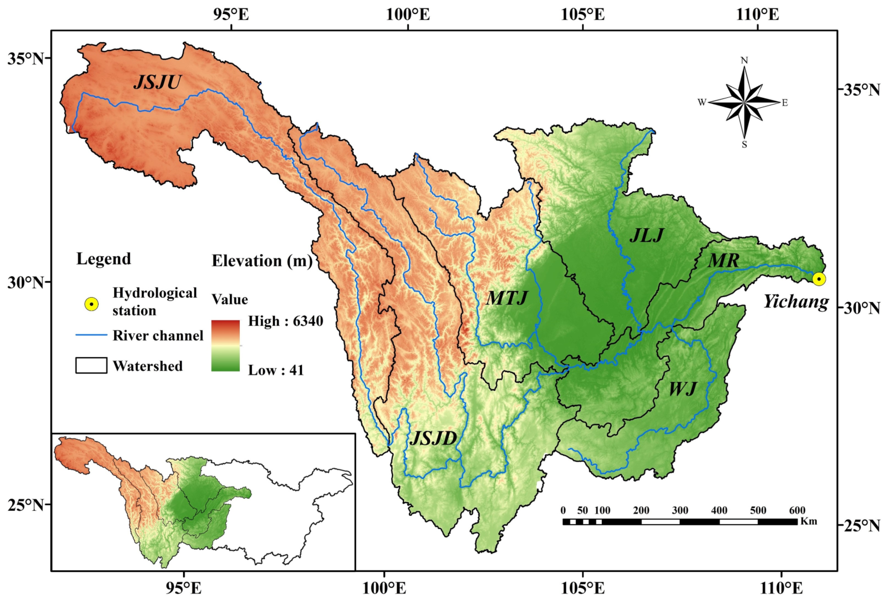
2.1. Study Area

The UYRB covers the region from the source to Yichang in Hubei province, which is nearly 1.00 million km2 [35,36] (Figure 1). The UYRB is characterized by a complex topography with varying slopes and a gradual decrease in elevation from west to east. Due to diverse landscapes and the obstructive effect of the plateau on the monsoon, a variety of climates have developed in the study area, including subtropical and humid climates in the east, arid climates in the northwest, and subtropical monsoon climates in the south. Precipitation is unevenly distributed during the year and concentrated in summer, with a gradual increase from northwest to southeast [35].
The spatial distribution of meteorological stations in the UYRB is shown in Figure 1. Yichang hydrological station, at the outlet of the UYRB, is located approximately 40 km downstream of the Three Gorges Dam [35]. The UYRB is divided into six sub-watersheds (Figure 1), including the Jinshajing River upstream (JSJU), the Jinshajiang River downstream (JSJD), the MinTuojiang River (MTJ), the Jialingjiang River (JLJ), the Wujiang River (WJ), and the Main River (MR).

2.2. Data Sources

The necessary data of the InVEST model include precipitation (PRE), potential evapotranspiration (PET), land use/cover, digital elevation model (DEM), plant available water capacity (PAWC), soil data, and biophysical tables. Runoff observations from the Yichang hydrological station were used to calibrate the water yield module. In addition, the normalized difference vegetation index (NDVI), the annual average temperature (TMP), and the relative humidity (RHU) were collected to analyze the potential driving factors of WCF. The details are shown in Table 1.

2.3. Methods

The flowchart of the investigation is shown in Figure 2. It consists of three parts, including calculation of WCF, spatiotemporal heterogeneity analysis, and driving factors analysis. The specific methods are presented below in detail.

2.3.1. The InVEST Water Yield Model

The InVEST is a collection of models used to evaluate multiple ecosystem services [19,39]. The water yield model is an important module of the InVEST model, which utilizes a raster cell and is founded on the Budyko hydrothermal coupling equilibrium. Water yield is calculated using input data such as precipitation, evapotranspiration, plant water availability content, soil depth, and land use/ land cover. The formula is as follows:
Y ( x ) = ( 1 A E T ( x ) P ( x ) ) × P ( x )
where Y ( x ) (mm) denotes the annual water yield for pixel x; A E T ( x ) (mm) denotes the annual actual evapotranspiration for pixel x, and P ( x ) (mm) denotes the annual precipitation on pixel x. A E T ( x ) P ( x ) is based on the expression of the Budyko curve proposed by Fu [40] and Zhang et al. [41]:
A E T ( x ) P ( x ) = 1 + P E T ( x ) P ( x ) [ 1 + ( P E T ( x ) P ( x ) ) ω ] 1 / ω
where P E T ( x ) (mm) denotes the potential evapotranspiration, and ω ( x ) denotes a nonphysical parameter that characterizes the natural climate–soil properties. Furthermore, the details are shown as follows:
P E T ( x ) = K c × E T 0 ( x )
where E T 0 ( x ) (mm) denotes the reference evapotranspiration, and Kc denotes the plant (vegetation) evapotranspiration coefficient associated with LULC x:
E T 0 ( x ) = 0.0023 × R a × ( T m e a n + 17.8 ) × T max T min
where Ra [MJ/(m2·d)] denotes radiation at the top of the atmosphere, Tmean (°C) denotes the mean temperature, Tmax (°C) denotes the maximum temperature, and Tmin (°C) denotes the minimum temperature [42]:
ω ( x ) = Z × A W C ( x ) P ( x ) + 1.25
where Z (1–30), known as the “seasonality factor”, denotes the synthesis of hydrogeological features and regional precipitation characteristics [3,4]. AWC(x) denotes the plant’s available water content (mm) for pixel x and is obtained by calculating the PAWC, the vegetation rooting depth (root.depth), and root restricting layer depth (rest.layer.depth). The equation is as follows:
A W C ( x ) = M i n ( r o o t . d e p t h . r e s t , r e s t . l a y e r . d e p t h ) × P A W C
The biophysical coefficients used in the InVEST model are shown in Table 2.
The accuracy of the model was assessed using the root mean square error (RMSE) and Nash–Sutcliffe efficiency (NSE) [4,43]. Generally, 0.75 < NSE ≤ 1.00 indicates very good results; 0.65 < NSE ≤ 0.75 indicates good results [43].

2.3.2. Calculation of WCF

Water yields can be obtained through the water yield module in the InVEST model, and then WCF (Retention) is calculated based on the topographic index (TI), the velocity coefficient (Velocity), and the saturated soil hydraulic conductivity (Ksat). The important grades of WCF were assessed based on the natural break method [44]. The WCF is defined as follows:
R e t e n t i o n = m i n ( 1 , 249 V e l o c i t y ) × m i n ( 1 , 0.9 × T I 3 ) × m i n ( 1 , K s a t 300 ) × Y i e l d

2.3.3. Emerging Hot Spot Analysis (EHSA)

EHSA is a geospatial tool, which integrates temporal column information into general hot spot analysis [21,45], that could identify the spatial and temporal heterogeneity of WCF more accurately and comprehensively. EHSA requires a space–time cube, which is a netCDF file containing x, y, and z (time) dimensions. The yearly data in each geographic grid were combined to generate a space–time cube that is used to operate EHSA. Then, the neighborhood distance and timestep parameters were set to the desired values, and Getis–Ord Gi* statistics were computed for each bar. The geographic resolution of the supplied data determines the neighborhood distance, and the timestep is shown for each year. Finally, the hot (or cold) spot trends were determined using the Mann–Kendall trend test [46]. Via EHSA, the spatiotemporal trends are displayed as hot (cold) spots. Up to 17 patterns are further summarized to distinguish whether the hot (cold) spots are new, persistent, sporadic, intensifying, consecutive, diminishing, oscillating, historical, or no pattern detected. EHSA is helpful for clarifying the aggregation patterns of WCF, and it is performed using ArcGIS Pro 2.5.

2.3.4. Geographical Detector Model (GDM)

The GDM is a novel spatial variation analysis method for discovering spatially stratified heterogeneity and detecting potential driving factors [30,47]. The fundamental theoretical assumption of its theory is that if independent variables have a substantial impact on the dependent variable, they ought to have a comparable geographical distribution. GDM was applied to detect the driving factors of the WCF in UYRB. Factor detection is used to rank the explanatory degree of individual factors. Furthermore, interaction detection identifies the joint effect of different factors.
The factor detector is evaluated according to the q statistic:
q = 1 h = 1 L N h σ h 2 N σ 2
where h = 1 , , L denotes the strata of variable Y or factor X; Nh refers to the numbers of units in strata h; N refers to the numbers of units in the entire region; σ h 2 denotes the variance in Y for strata h; σ 2 denotes the variance in Y for the entire region. The value range of q is [0, 1], and the explanatory power of X for Y increases with the value of q [48].
The interaction detector makes it possible to identify whether driving factors X1 and X2 function jointly to increase the explanatory degree of dependent variable Y or whether their effects on Y are independent of one another [32]. The interaction categories and relationships of the two factors are shown in Table 3.

3. Results

3.1. Simulation and Validation of the InVEST

When the calculated water yield and observed runoff fit together the best and the model’s simulation effect was at its best (NSE = 0.76, RMSE = 2.51), the Z value was calibrated to 1.10 (Figure 3). Based on the criteria, the validity and suitability of the InVEST model for this investigation were confirmed.

3.2. Spatial Patterns of Multi-Year Average WCF

The geographical patterns of WCF and multi-year average water yield from 1991 to 2020 were similar. A decreasing tendency from the southeast to the northwest was visible in the average annual WCF during the 1991–2020 period, and the difference between the maximum value and the minimum value is 1326.22 mm (Figure 4b). The average annual (1991–2020) water yield, precipitation, and actual evapotranspiration (AET) had highly variable regional distribution patterns that were comparable to the WCF, indicating an inclination to increase from the northwest to the southeast (Figure 4a,c,d). The MR watershed, WJ watershed, and downstream of the MTJ watershed contained most of the high-value regions, where rainfall was abundant, and the agricultural acreage was relatively wide, resulting in the easy formation of runoff. The median-value areas were located in the middle of the sub-watershed, with higher forest coverage. Lower water production is the result of precipitation being intercepted by the forest canopy, deadfall layer, and soil layer. The source section of the sub-watershed was where the low-value regions were concentrated, with a small amount of precipitation (the minimum precipitation was 229.18 mm) and steep terrain.
Figure 5 presents the regional distribution and area proportion of the WCF’s important grades. The largest proportion is grade II and grade III, 30.63% and 28.12%, respectively. The center of the study area is where the intermediate-grade regions are located. The smallest proportion, 7.98%, of grade IV is located downstream of the study area. For a more detailed understanding, the distribution within each sub-watershed was analyzed. The majority of areas within the JSJU watershed were grade I and grade II. In the MR and WJ watersheds, grade IV and grade V were dominant. The JSJD, MTJ, and JLJ watersheds, which make up the study area’s central region, were primarily dominated by grade II and grade III. However, the fact that the lower portions of the MTJ watershed include a sizable percentage of grade V cannot be ignored. The regions with low water conservation importance grades provide important water resources for economic and social development, which should be protected with emphasis.

3.3. Inter-Annual Variation of WCF

Figure 6 exhibits the average annual WCF of the UYRB and six sub-watersheds from 1991 to 2020. The average annual WCF of the UYRB displays an increasing trend. The average annual increase rate was 1.48 mm, with the highest value of 454.27 mm (1998) and the lowest value of 280.65 mm (2006). There was an elevated trend in all watersheds, except for the JSJD watershed. The JLJ watershed showed the fastest increase with a rate of 3.99 mm/a, while the JSJD watershed was the only sub-watershed that showed a declining trend, decreasing at a rate of 0.45 mm/a. In addition, the inter-annual variation in the WCF of each watershed was significant. The high values frequently occurred in 1993, 1998, 2008, and 2015, while the low values were in 2006, 2011, and 2019.
The temporal trends of WCF from 1991 to 2020 were analyzed using the inter-annual variation slope (Figure 7). In the downstream of JLJ and MTJ watersheds, the slope reached over 3 mm/a, which indicates a considerable increase in WCF in this region during the previous 30 years. Despite the fact that the WCF in the majority of the UYRB exhibited an upward trend, there were variations in the increased amplitude of certain watersheds and even a drop in certain watersheds, especially in the JSJD watershed. In addition, at the Yangtze River’s source area, the WCF showed a relatively obvious trend of increase. This may be ascribed to the Three-River Headwater Region’s ecological protection effort (e.g., returning pasture to grass, returning farmland to forest, and ecological transplantation).
The coefficient of variation (Cv) values of the WCF are shown in Figure 8. The Cv values of the MTJ and MR watersheds were relatively low, which indicated that these regions experienced slight variations during the past 30 years. In contrast, the high Cv values (>2) occurred in the source area of the Yangtze River, which represented a greater degree of fluctuation. Interestingly, both the high-value area of Cv and slope occurred in the Yangtze River’s source area. This showed that the WCF was significantly influenced by human activities, such as ecological restoration projects. In addition, since the Cv value is characterized as the standard deviation to mean ratio, it is inevitably affected by the average WCF. Therefore, Cv exhibited its maximum value at the source of the UYRB, where the average WCF was low. At the sub-watershed scale, the JSJU watershed had the largest Cv value. The JSJD and JLJ watersheds exhibited Cv values that fell in the middle. The large areas with small Cv values existed in MTJ, MR, and WJ watersheds. It can be demonstrated that the spatial distribution of Cv values was similar to that of WCF, which indicates that the average WCF has a non-negligible influence on the Cv value.

3.4. Spatiotemporal Heterogeneity of WCF

In the EHSA, low WCF values are aggregated as a cold spot, while high WCF values are aggregated as a hot spot. The spatial patterns and statistical analysis results for each pattern are depicted in Figure 9 and Figure 10. The distribution of cold spots and hot spots is relatively independent. The hot spots were primarily located in the east, while the cold spots were mostly located in the west. In addition, the upper reaches of the MTJ and JLJ watersheds also exhibited cold spot aggregations (Figure 9). We detected a total of 16 EHSA patterns, except for “New Hot Spot”.
Among the hot spot patterns, “Persistent Hot Spot” (125.13‰) and “Sporadic Hot Spot” (104.86‰) accounted for the majority. The MR, WJ, and lower MTJ watersheds were characterized by a “Persistent Hot Spot”, which showed statistically significant lower WCFs. The adjacent areas of the JLJ, MTJ, and MR watersheds showed an “Intensifying Hot Spot” (28.39‰), which indicated that the high WCF gradually increased. A “Sporadic Hot Spot” was distributed in the eastern region of the research area dispersedly. Cold spot patterns were located in the western region, including “Intensifying Cold Spot”, “Persistent Cold Spot”, “Diminishing Cold Spot”, “Sporadic Cold Spot”, and “Oscillating Cold Spot” patterns. The upper reaches of the three watersheds (JSJU, MTJ, and JLJ) were covered by a “Persistent Cold Spot” (124.06‰). In the center sections of the Jinshajiang River basin, a “Sporadic Cold Spot” (170.06‰) indicated weak WCF but was not statistically significant. However, an “Intensifying Cold Spot” (32.51‰) represented the yearly decline in the WCF. The lower JSJD watershed was characterized by an “Oscillating Cold Spot” (30.12‰), indicating that these areas were the lower-value regions in the UYRB despite having some higher-value periods. The source area of the JSJU watershed was covered by a large number of “Diminishing Cold Spots” (38.24‰), meaning that the WCF of this area, although weak, had been slowly increasing during the 1991–2020 period. Approximately one-third of the study area was detected as “No Pattern Detected” (341.92‰), indicating the absence of any statistically significant changes. The WCF of the UYRB exhibited strong spatiotemporal heterogeneity, with cold spot patterns (395.07‰) accounting for more than the hot spot patterns (263.02‰). Hence, it is worthwhile to conduct further attribution analysis.

3.5. Analysis of Driving Factors on WCF

The inter-annual trend of driving factors is shown in Figure 11. With an overall fluctuating increasing tendency and an average rate of 2.23 mm/a, the multi-year average precipitation was 829.84 mm. The average mean temperature of the UYRB ranged between 6.85 °C and 8.08 °C, increasing significantly at a rate of 0.28 °C/10a (1991–2020). The average relative humidity was 68.97, representing a clear increasing trend. The potential evapotranspiration and actual evapotranspiration exhibited increasing trends at rates of 1.16 mm/a and 0.38 mm/a, respectively. In detail, the ratio of actual evapotranspiration to precipitation was approximately 0.46, indicating that nearly half of the area’s precipitation was directly returned to the atmosphere via evapotranspiration. For NDVI, the increasing trend was the most pronounced, with annual averages between 0.56 and 0.69, indicating that the UYRB is becoming “greener” year by year.
In general, the agglomeration pattern of WCF is driven by a combination of many driving factors. GDM was employed to identify the driving factors and their explanatory power relative to WCF. Since the driver factors applied in GDM must be categorical variables, the natural breaks classification method was used to transform the original dependent variables (including PRE, RHU, DEM, TMP, PET, AET, NDVI, SD, PAWC, Ksat, and TI) from numerical variables to categorical variables. Figure 12 shows the q-values of driving factors for the WCF in the UYRB from 1991 to 2020. The rank of q-statistic values was as follows: PRE (0.701) > RHU (0.527) > DEM (0.409) > TMP (0.387) > PET (0.311) > AET (0.254) > NDVI (0.250) > SD (0.132) > PAWC (0.106) > Ksat (0.086) > TI (0.061), with q-values significant at the 1% level (p < 0.01). The WCF was overwhelmingly determined by PRE, RHU, and DEM.
Furthermore, the interaction detection results for the WCF of UYRB in 1991–2020 are illustrated in Figure 13. As we summarized from the graph, every detection factor was not independent. Further information showed that the q-values of double factors were larger than those of individual factors, which suggested that each pair of factors contributes to the WCF in an interactive way [39]. When Ksat was analyzed in combination with additional driving factors, the q-value was more than the sum of the two single factors’ q-values, representing nonlinear enhancements. The q-value of each pair of factor interactions for other driving factors was higher than the q-value of any single factor, but it was lower than the total of the q-values of the two single factors. Therefore, the interaction relationships of these driving factors exhibited bivariate enhanced properties when affecting the WCF. In detail, the interaction effect of PRE and Ksat, q(PRE∩Ksat), exhibited the maximum value (q = 0.84), indicating that the combined force is the strongest, followed by the combination of PRE and AET, q(PRE∩AET) = 0.78, and the combination of PRE and TMP, q(PRE∩TMP) = 0.75. Hence, the interactions between PRE and other factors were the strongest, indicating that PRE was the most crucial driving factor. In conclusion, the interaction effect of two driving factors played a more crucial role in influencing WCF than the single factor separately.

4. Discussion

4.1. Spatiotemporal Heterogeneity of the WCF in the UYRB

WCF provides water resources for the ecosystem internally and externally by storing precipitation in the forest canopy, deadfall, and soil layer at a specific spatiotemporal scale [4]. In the UYRB, the WCF shows low patterns in the northwest and high patterns in the southeast, with an increasing trend from 1991 to 2020. It is worth noting that the research region is mountainous in the west, and the “Sichuan basin” is located in the east, which also contributes to the spatial distribution of WCF. The excellent hydrothermal conditions at low-elevation areas allow for lush and well-rooted vegetation, which complements the relatively gentle terrain and will benefit water conservation [4]. However, the fragile ecological structure and cold climate at high altitudes make surface water highly susceptible to loss and low water conservation potential [49]. The areas with a high WCF, including the WJ watershed, MR watershed, and downstream of the MTJ watershed and JLJ watershed, were characterized by relatively higher proportions of vegetation cover and abundant precipitation [50]. Moreover, high-value regions are characterized by the presence of extensive forests and grasslands with greater soil depths, as well as vegetation and deadfall layers that effectively intercept and store precipitation [51]. On the contrary, the regions with low WCF had poor precipitation and vegetation cover conditions and shallow soil depths, resulting in a weak ability to conserve water. In mountainous areas with shallow soil depths and sparse vegetation, precipitation easily forms runoffs rather than be stored [52]. In areas with limited precipitation and cold temperatures, where alpine meadows are the predominant community, the WCF is weaker. High-elevation soils have shallower soils and a poorer ability to retain water due to the low temperature that restricts plant growth and soil formation [5]. This has also resulted in low WCF in the western part of the UYRB.
Our analysis revealed that the WCF of the Three-River Headwater Region, situated in the research area’s source region, showed the most significant change (Figure 7 and Figure 8) and exhibited an increasing trend [18]. This suggests that the national policy may potentially encourage an increase in WCF. The Overall Planning of Ecological Protection and Construction of the Three-River Headwaters Nature Reserve in Qinghai Province, approved in 2005, involves various plans, such as returning pasture to grass [18], returning farmland to forest, and ecological transplantation. The WCF has substantially improved since the Three-River Headwater source’s ecological preservation initiative was put into action, which is in accordance with the findings of previous investigations [49,53]. On the other hand, the worsening warming of the climate has led to an increase in glacier meltwater [54], and the implementation of measures such as artificial rainfall has also increased precipitation [55]. After 2005, the climatic characteristics of the source area have tended to be warmer and more humid [56]. Here, the amplifying effects [57] of climate change and human activities contribute to the improvements in WCF. Therefore, the improvements in WCF in the western region require more attention. Rigorous forest protection and light anthropogenic disturbance (e.g., cultivation of cropland and overgrazing) will help improve WCF [58]. Additionally, the suitable plant type and rational ecological design (selecting logging and thinning) could improve the ability of ecosystems to combat climate change [57] and thus improve the stability of WCF.

4.2. Main Driving Factors of WCF Change

WCF refers to storing water resources [13] and, at the same time, replenishing groundwater and runoff during dry periods [4]. Therefore, WCF involves multiple water cycle processes and is influenced by multiple drivers. The most significantly correlated drivers were PRE, RHU, DEM, and TMP [3,4]. Generally, compared to single-factor analysis, multifactor analysis is typically more logical and scientific. Via interaction detection analysis, it was observed that PRE and Ksat had the greatest effect on WCF when they affected WCF together (Figure 13). Apparently, higher precipitation in conjunction with a higher Ksat leads to greater infiltration of water into the soil, resulting in increased water storage [59]. Moreover, the combination of PRE and evapotranspiration also had a prominent impact on WCF. Due to the participation in terrestrial water cycle processes, strong evapotranspiration can lead to less efficient conversion of precipitation into water. Both PRE and evapotranspiration significantly affected the WCF according to the water balance [60], which was verified in this study (Figure 12). On the other hand, TMP also affects WCF by influencing multiple processes (e.g., water cycle and plant growth). Good hydrothermal conditions contribute to the growth of vegetation [61,62]. Studies have revealed that climatic warming hastens the breakdown of soil organic and lengthens the vegetative growth cycle [62]. Meanwhile, the increase in TMP accelerated the thawing of glaciers [63] and the melting of ground ice [28] in the study region, leading to enhanced recharge, which is beneficial to the improvement of WCF. However, anomalous atmospheric warming can lead to catastrophic debris flow that disrupt overall ecosystem services [7]. NDVI, as a reflection of vegetation condition, also influences WCF along with other driving factors. Regions covered with vegetation, such as grasslands and forests, can intercept more water due to the presence of branches and roots [17]. Long-term vegetative cover also facilitates soil evolution, which in turn benefits water absorption and storage [64]. Hence, PRE, TMP, and NDVI have comprehensive effects on the WCF. In addition, WCF may be affected by species, forest types, climate types, and hydrological regimes [65]. Soil moisture, as an important water resource component, has a direct impact on the WCF. The current high-resolution soil moisture products generated by remote sensing satellites provide new ideas for assessing and analyzing the WCF and offer an efficient data source for large-scale and high temporal resolution assessments [66,67,68,69]. Therefore, improving WCF requires maintaining a healthy forest structure and a wide variety of species [57]. In conclusion, the WCF of the UYRB is complexly influenced by multiple driving factors [5,18]. We could gradually deepen our understanding of the driving mechanism by continuously analyzing the underlying influencing factors.

4.3. Limitations and Uncertainties

Although this study analyzed the spatiotemporal evolution and driving factors of the WCF in the UYRB based on emerging and comprehensive methods, there were still some limitations and uncertainties. (1) First, despite the InVEST model’s proven validity in assessing the WCF [19,39], the exclusion of glaciers and frozen soil may have an impact on the calculation of WCF [18]. Although the resolution of the input data used in this study (1000 m × 1000 m) proved to be a satisfactory performance resolution for the model [70], high-precision materials may provide better results. (2) Second, GDM needs to discretize the input data using classifications, such as natural break points [31], the standard deviation method [71], or equal spacing methods [72]. Different methods may result in different input errors. (3) Third, the analysis of the driving factors and their interactions with WCF was carried out statistically in this study, and specific mechanistic explanations require further research. Given the limitations, future research should explore the specific influence process and mechanism of the driver factors on WCF using more comprehensive and detailed monitoring data.

5. Conclusions

This study aims to investigate the spatiotemporal heterogeneity of the WCF in UYRB and its driving factors. For this goal, the WCF was assessed using the InVEST model, and its cold (hot) aggregation patterns were detected via EHSA. Furthermore, the driving factors of WCF and their interactions were explored scientifically based on GDM. The application of EHSA allows us to detect the state of the WCF at specific locations and its temporal patterns, and GDM helps us to analyze the interactive effects of different driving factors on WCF. This study can provide a basis for the development of differentiated water resources management measures. The key conclusions are as follows.
(1)
The inter-annual variation of the WCF in UYRB was significant. During the 1991–2020 period, the WCF of the study region showed a slight increase integrally, with a growth rate of 1.48 mm/a. The areas with the fastest growing rate were located in the JLJ and MR watersheds, reaching 3.99 mm/a and 3.15 mm/a, respectively. The JSJD watershed showed a decreasing trend at a rate of −0.85 mm/a, indicating that measures are needed for alleviation. The JSJU watershed had a significant improvement in WCF, with high slope and Cv values.
(2)
The WCF of UYRB exhibited significant spatial heterogeneity that gradually increased from the northwest to the southeast. Specifically, in the eastern region, the WCF was strong and belonged to the hot spots. On the contrary, the fragile area of the WCF was located in the western portion of the study region, including the JSJU watershed, the JSJD watershed, the headwaters of the MTJ watershed, and the JLJ watershed. The western region is a priority area for implementing WCF enhancement strategies.
(3)
Among all selected driving factors, PRE (q-value = 0.701) was the factor with the highest level of explanatory power affecting the spatial differentiation of WCF in the UYRB, followed by RHU (q-value = 0.527), DEM (q-value = 0.409), TMP (q-value = 0.387), and PET (q-value = 0.311). Moreover, the explanatory power of the factor’s interactions relative to the spatial heterogeneity of WCFs was higher than the single-factor results. The interactions of multiple driving factors should be considered in improving WCF.

Author Contributions

C.L.; methodology, software, investigation, data analysis, writing—original draft, review, and editing. L.Z. (Lei Zou); methodology, resources, conceptualization, supervision, writing—review and editing. J.X.; formal analysis, methodology. X.C.; writing—review and editing. L.Z. (Lingfeng Zuo); writing—review and editing. J.Y.; writing—review and editing. All authors have read and agreed to the published version of the manuscript.

Funding

This research was funded by the Strategic Priority Research Program of the Chinese Academy of Sciences (No. XDA23040304), the National Natural Science Foundation of China (No. 41890823, 42101043), and the Special Fund for Science and Technology Innovation Strategy of Guangdong Province (sky2023-05). We are very grateful to the editors and the anonymous reviewers for their constructive suggestions that helped us to improve the manuscript.

Data Availability Statement

The data presented in this study are available on request from the corresponding author.

Conflicts of Interest

The authors declare no conflict of interest.

References

  1. Daily, G.C.; Matson, P.A. Ecosystem services: From theory to implementation. Proc. Natl. Acad. Sci. USA 2008, 105, 9455–9456. [Google Scholar] [CrossRef] [PubMed]
  2. Wallace, K.J. Classification of ecosystem services: Problems and solutions. Biol. Conserv. 2007, 139, 235–246. [Google Scholar] [CrossRef]
  3. Li, M.; Liang, D.; Xia, J.; Song, J.; Cheng, D.; Wu, J.; Cao, Y.; Sun, H.; Li, Q. Evaluation of water conservation function of Danjiang River Basin in Qinling Mountains, China based on InVEST model. J. Environ. Manag. 2021, 286, 112212. [Google Scholar] [CrossRef] [PubMed]
  4. Wang, Y.; Ye, A.; Peng, D.; Miao, C.; Di, Z.; Gong, W. Spatiotemporal variations in water conservation function of the Tibetan Plateau under climate change based on InVEST model. J. Hydrol. Reg. Stud. 2022, 41, 101064. [Google Scholar] [CrossRef]
  5. Xu, H.-j.; Zhao, C.-y.; Wang, X.-p.; Chen, S.-y.; Shan, S.-y.; Chen, T.; Qi, X.-l. Spatial differentiation of determinants for water conservation dynamics in a dryland mountain. J. Clean. Prod. 2022, 362, 132574. [Google Scholar] [CrossRef]
  6. Sun, G.; Zhang, L.; Wang, Y. On accurately defining and quantifying the water retention services of forests. Acta Ecol. Sin. 2023, 43, 9–25. (In Chinese) [Google Scholar] [CrossRef]
  7. Shugar, D.H.; Jacquemart, M.; Shean, D.; Bhushan, S.; Upadhyay, K.; Sattar, A.; Schwanghart, W.; McBride, S.; Van Wyk de Vries, M.; Mergili, M.; et al. A massive rock and ice avalanche caused the 2021 disaster at Chamoli, Indian Himalaya. Science 2021, 373, 300–306. [Google Scholar] [CrossRef] [PubMed]
  8. Mahmoud, S.H.; Gan, T.Y. Impact of anthropogenic climate change and human activities on environment and ecosystem services in arid regions. Sci. Total Environ. 2018, 633, 1329–1344. [Google Scholar] [CrossRef]
  9. Cheng, H.; Hu, Y.; Zhao, J. Meeting China’s water shortage crisis: Current practices and challenges. Environ. Sci. Technol. 2009, 43, 240–244. [Google Scholar] [CrossRef]
  10. Wen, X.; Theau, J. Spatiotemporal analysis of water-related ecosystem services under ecological restoration scenarios: A case study in northern Shaanxi, China. Sci. Total Environ. 2020, 720, 137477. [Google Scholar] [CrossRef]
  11. Yang, D.; Liu, W.; Tang, L.; Chen, L.; Li, X.; Xu, X. Estimation of water provision service for monsoon catchments of South China: Applicability of the InVEST model. Landsc. Urban Plan. 2019, 182, 133–143. [Google Scholar] [CrossRef]
  12. Lai, M.; Wu, S.; Dai, E.; Yin, Y.; Zhao, D. The Indirect Value of Ecosystem Services in the Three-River Headwaters Region. J. Nat. Resour. 2013, 28, 39–50. (In Chinese) [Google Scholar]
  13. Zhang, B.; Li, W.; Xie, G.; Xiao, Y. Water conservation of forest ecosystem in Beijing and its value. Ecol. Econ. 2010, 69, 1416–1426. [Google Scholar] [CrossRef]
  14. Abouabdillah, A.; White, M.; Arnold, J.G.; De Girolamo, A.M.; Oueslati, O.; Maataoui, A.; Lo Porto, A. Evaluation of soil and water conservation measures in a semi-arid river basin in Tunisia using SWAT. Soil Use Manag. 2014, 30, 539–549. [Google Scholar] [CrossRef]
  15. Wu, Q.; Song, J.; Sun, H.; Huang, P.; Jing, K.; Xu, W.; Wang, H.; Liang, D. Spatiotemporal variations of water conservation function based on EOF analysis at multi time scales under different ecosystems of Heihe River Basin. J. Environ. Manag. 2023, 325, 116532. [Google Scholar] [CrossRef]
  16. Nie, Y. A Study of the Water Conservation of Qilian Mountains based on surface energy and SCS model. Earth Sci. Front. 2010, 17, 269–275. (In Chinese) [Google Scholar]
  17. Jia, G.; Hu, W.; Zhang, B.; Li, G.; Shen, S.; Gao, Z.; Li, Y. Assessing impacts of the Ecological Retreat project on water conservation in the Yellow River Basin. Sci. Total Environ. 2022, 828, 154483. [Google Scholar] [CrossRef]
  18. Xue, J.; Li, Z.; Feng, Q.; Gui, J.; Zhang, B. Spatiotemporal variations of water conservation and its influencing factors in ecological barrier region, Qinghai-Tibet Plateau. J. Hydrol. Reg. Stud. 2022, 42, 101164. [Google Scholar] [CrossRef]
  19. Dennedy-Frank, P.J.; Muenich, R.L.; Chaubey, I.; Ziv, G. Comparing two tools for ecosystem service assessments regarding water resources decisions. J. Environ. Manag. 2016, 177, 331–340. [Google Scholar] [CrossRef]
  20. Daneshi, A.; Brouwer, R.; Najafinejad, A.; Panahi, M.; Zarandian, A.; Maghsood, F.F. Modelling the impacts of climate and land use change on water security in a semi-arid forested watershed using InVEST. J. Hydrol. 2021, 593, 125621. [Google Scholar] [CrossRef]
  21. Fan, P.Y.; Chun, K.P.; Mijic, A.; Tan, M.L.; Yetemen, O. Integrating the Budyko framework with the emerging hot spot analysis in local land use planning for regulating surface evapotranspiration ratio. J. Environ. Manag. 2022, 316, 115232. [Google Scholar] [CrossRef] [PubMed]
  22. Fan, P.Y.; Chun, K.P.; Mijic, A.; Tan, M.L.; He, Q.; Yetemen, O. Quantifying land use heterogeneity on drought conditions for mitigation strategies development in the Dongjiang River Basin, China. Ecol. Indic. 2021, 129, 107945. [Google Scholar] [CrossRef]
  23. Wan, C.; Roy, S.S. Geospatial characteristics of fire occurrences in southern hemispheric Africa and Madagascar during 2001–2020. J. For. Res. 2022, 34, 553–563. [Google Scholar] [CrossRef]
  24. Khan, S.D.; Gadea, O.C.A.; Tello Alvarado, A.; Tirmizi, O.A. Surface Deformation Analysis of the Houston Area Using Time Series Interferometry and Emerging Hot Spot Analysis. Remote Sens. 2022, 14, 3831. [Google Scholar] [CrossRef]
  25. Satalova, B.; Kenderessy, P. Assessment of water retention function as tool to improve integrated watershed management (case study of Poprad river basin, Slovakia). Sci. Total Environ. 2017, 599–600, 1082–1089. [Google Scholar] [CrossRef] [PubMed]
  26. Chen, J.; Zhang, J.; Peng, J.; Zou, L.; Fan, Y.; Yang, F.; Hu, Z. Alp-valley and elevation effects on the reference evapotranspiration and the dominant climate controls in Red River Basin, China: Insights from geographical differentiation. J. Hydrol. 2023, 620, 129397. [Google Scholar] [CrossRef]
  27. Hu, W.; Li, G.; Li, Z. Spatial and temporal evolution characteristics of the water conservation function and its driving factors in regional lake wetlands—Two types of homogeneous lakes as examples. Ecol. Indic. 2021, 130, 108069. [Google Scholar] [CrossRef]
  28. Wu, J.; Sheng, Y.; Wu, Q.; Li, J.; Zhang, X. Discussion on possibilities of taking ground ice in permafrost as water sources on the Qinghai-Tibet Plateau during climate warming. Sci. Cold Arid. Reg. 2009, 1, 322–328. [Google Scholar]
  29. Hu, W.; Li, G.; Gao, Z.; Jia, G.; Wang, Z.; Li, Y. Assessment of the impact of the Poplar Ecological Retreat Project on water conservation in the Dongting Lake wetland region using the InVEST model. Sci. Total Environ. 2020, 733, 139423. [Google Scholar] [CrossRef]
  30. Wang, J.F.; Li, X.H.; Christakos, G.; Liao, Y.L.; Zhang, T.; Gu, X.; Zheng, X.Y. Geographical Detectors-Based Health Risk Assessment and its Application in the Neural Tube Defects Study of the Heshun Region, China. Int. J. Geogr. Inf. Sci. 2010, 24, 107–127. [Google Scholar] [CrossRef]
  31. Ding, Y.; Zhang, M.; Qian, X.; Li, C.; Chen, S.; Wang, W. Using the geographical detector technique to explore the impact of socioeconomic factors on PM2.5 concentrations in China. J. Clean. Prod. 2019, 211, 1480–1490. [Google Scholar] [CrossRef]
  32. Xu, M.; Bao, C. Quantifying the spatiotemporal characteristics of China’s energy efficiency and its driving factors: A Super-RSBM and Geodetector analysis. J. Clean. Prod. 2022, 356, 131867. [Google Scholar] [CrossRef]
  33. Feng, R.; Wang, F.; Wang, K. Spatial-temporal patterns and influencing factors of ecological land degradation-restoration in Guangdong-Hong Kong-Macao Greater Bay Area. Sci. Total Environ. 2021, 794, 148671. [Google Scholar] [CrossRef] [PubMed]
  34. Kong, L.; Wang, Y.; Zheng, H.; Xiao, Y.; Xu, W.; Zhang, L.; Xiao, Y.; Ouyang, Z. A method for evaluating ecological space and ecological conservation redlines in river basins: A case of Yangtze River Basin. Acta Ecol. Sin. 2019, 39, 835–843. (In Chinese) [Google Scholar] [CrossRef]
  35. Wang, A.; Yang, D.; Tang, L. Spatiotemporal variation in nitrogen loads and their impacts on river water quality in the upper Yangtze River basin. J. Hydrol. 2020, 590, 125487. [Google Scholar] [CrossRef]
  36. Wang, T.; Shi, R.; Yang, D.; Yang, S.; Fang, B. Future changes in annual runoff and hydroclimatic extremes in the upper Yangtze River Basin. J. Hydrol. 2022, 615, 128738. [Google Scholar] [CrossRef]
  37. Gupta, S.; Lehmann, P.; Bonetti, S.; Papritz, A.; Or, D. Global Prediction of Soil Saturated Hydraulic Conductivity Using Random Forest in a Covariate-Based GeoTransfer Function (CoGTF) Framework. J. Adv. Model. Earth Syst. 2021, 13, e2020MS002242. [Google Scholar] [CrossRef]
  38. Zhou, W.; Liu, G.; Pan, J.; Feng, X. Distribution of available soil water capacity in China. J. Geogr. Sci. 2005, 15, 3–12. [Google Scholar] [CrossRef]
  39. Cong, W.; Sun, X.; Guo, H.; Shan, R. Comparison of the SWAT and InVEST models to determine hydrological ecosystem service spatial patterns, priorities and trade-offs in a complex basin. Ecol. Indic. 2020, 112, 106089. [Google Scholar] [CrossRef]
  40. Fu, B. On the calculation of the evaporation from land surface. Chin. J. Atmos. Sci. 1981, 1, 23–32. (In Chinese) [Google Scholar]
  41. Zhang, L.; Hickel, K.; Dawes, W.R.; Chiew, F.H.S.; Western, A.W.; Briggs, P.R. A rational function approach for estimating mean annual evapotranspiration. Water Resour. Res. 2004, 40. [Google Scholar] [CrossRef]
  42. Peng, S.; Ding, Y.; Wen, Z.; Chen, Y.; Cao, Y.; Ren, J. Spatiotemporal change and trend analysis of potential evapotranspiration over the Loess Plateau of China during 2011–2100. Agric. For. Meteorol. 2017, 233, 183–194. [Google Scholar] [CrossRef]
  43. Luo, K. Response of hydrological systems to the intensity of ecological engineering. J. Environ. Manag. 2021, 296, 113173. [Google Scholar] [CrossRef]
  44. Xiao, S.; Zou, L.; Xia, J.; Dong, Y.; Yang, Z.; Yao, T. Assessment of the urban waterlogging resilience and identification of its driving factors: A case study of Wuhan City, China. Sci. Total Environ. 2023, 866, 161321. [Google Scholar] [CrossRef] [PubMed]
  45. Harris, N.L.; Goldman, E.; Gabris, C.; Nordling, J.; Minnemeyer, S.; Ansari, S.; Lippmann, M.; Bennett, L.; Raad, M.; Hansen, M.; et al. Using spatial statistics to identify emerging hot spots of forest loss. Environ. Res. Lett. 2017, 12, 024012. [Google Scholar] [CrossRef]
  46. ESRI. How Emerging Spatiotemporal Hot Spot Analysis Works. Available online: https://desktop.arcgis.com/zh-cn/arcmap/10.3/tools/space-time-pattern-mining-toolbox/learnmoreemerging.htm (accessed on 22 October 2022).
  47. Wang, J.-F.; Zhang, T.-L.; Fu, B.-J. A measure of spatial stratified heterogeneity. Ecol. Indic. 2016, 67, 250–256. [Google Scholar] [CrossRef]
  48. Wang, J.; Xu, C. Geodetector: Principle and Prospective. Acta Geogr. Sin. 2017, 72, 116–134. (In Chinese) [Google Scholar] [CrossRef]
  49. Wu, D.; Shao, Q.; Liu, J.; Cao, W. Assessment of Water Regulation Service of Forest and Grassland Ecosystem in Three-River Headwaters Region. Bull. Soil Water Conserv. 2016, 36, 207–210. (In Chinese) [Google Scholar] [CrossRef]
  50. Yi, L.; Sun, Y.; Yin, S.; Wei, X.; Ouyang, X. Spatial-temporal variations of vegetation coverage and its driving factors in the Yangtze River Basin from 2000 to 2019. Acta Ecol. Sin. 2023, 43, 798–811. [Google Scholar] [CrossRef]
  51. Zagyvai-Kiss, K.A.; Kalicz, P.; Szilágyi, J.; Gribovszki, Z. On the specific water holding capacity of litter for three forest ecosystems in the eastern foothills of the Alps. Agric. For. Meteorol. 2019, 278, 107656. [Google Scholar] [CrossRef]
  52. Wosten, J.H.M.; Pachepsky, Y.A.; Rawls, W.J. Pedptransfer functions: Bridging the gap between available basic soil data and missing soil hydraulic characteristics. J. Hydrol. 2001, 251, 123–150. [Google Scholar] [CrossRef]
  53. Jiang, Y.; Du, W.; Huang, J.; Zhao, H.; Wang, C. Analysis of vegetation changes in the Qilian Mountains during 2000–2015. J. Glaciol. Geocryol. 2017, 39, 1130–1136. (In Chinese) [Google Scholar] [CrossRef]
  54. Jiang, Y.; Li, S.; Shen, D.; Chen, W. Climate Change and Its Impact on the Regional Environment in the Source Regions of the Yangtze, Yellow and Lantsang Rivers in Qinghai-Tibetan Plateau during 1971–2008. J. Mt. Sci. 2012, 30, 461–469. (In Chinese) [Google Scholar] [CrossRef]
  55. Gong, j.; Zhang, Y.; Wang, Q.; Zhu, S.; Guo, S.; He, Y. Analysis on Artificial Precipitation Enhancement Potential of Aerial Cloud Water Resources and lts lmpact on the Ecological Environment in Sanjiangyuan. J. Qinghai Environ. 2020, 30, 82–90. (In Chinese) [Google Scholar]
  56. Yao, X.; Xie, Q.; Huang, Y. Advances and prospects on the study of precipitation in the Three-River-Source Region in China. Trans. Atmos. Sci. 2022, 45, 688–699. (In Chinese) [Google Scholar] [CrossRef]
  57. Zhang, M.; Liu, S.; Jones, J.; Sun, G.; Wei, X.; Ellison, D.; Archer, E.; McNulty, S.; Asbjornsen, H.; Zhang, Z.; et al. Managing the forest-water nexus for climate change adaptation. For. Ecol. Manag. 2022, 525, 120545. [Google Scholar] [CrossRef]
  58. Mina, M.; Bugmann, H.; Cordonnier, T.; Irauschek, F.; Klopcic, M.; Pardos, M.; Cailleret, M.; Brando, P. Future ecosystem services from European mountain forests under climate change. J. Appl. Ecol. 2017, 54, 389–401. [Google Scholar] [CrossRef]
  59. Maurya, S.; Srivastava, P.K.; Gupta, M.; Islam, T.; Han, D. Integrating Soil Hydraulic Parameter and Microwave Precipitation with Morphometric Analysis for Watershed Prioritization. Water Resour. Manag. 2016, 30, 5385–5405. [Google Scholar] [CrossRef]
  60. Or, D.; Lehmann, P. Surface Evaporative Capacitance: How Soil Type and Rainfall Characteristics Affect Global-Scale Surface Evaporation. Water Resour. Res. 2019, 55, 519–539. [Google Scholar] [CrossRef]
  61. Wang, J.; Rich, P.M.; Price, K.P. Temporal responses of NDVI to precipitation and temperature in the central Great Plains, USA. Int. J. Remote Sens. 2010, 24, 2345–2364. [Google Scholar] [CrossRef]
  62. Ren, Z.; Tian, Z.; Wei, H.; Liu, Y.; Yu, Y. Spatiotemporal evolution and driving mechanisms of vegetation in the Yellow River Basin, China during 2000–2020. Ecol. Indic. 2022, 138, 108832. [Google Scholar] [CrossRef]
  63. Liu, S.; Zhang, Y.; Zhang, Y.; Ding, Y. Estimation of glacier runoff and future trends in the Yangtze River source region, China. J. Glaciol. 2017, 55, 353–362. [Google Scholar] [CrossRef]
  64. Zhang, Y.; Du, J.; Guo, L.; Sheng, Z.; Wu, J.; Zhang, J. Water Conservation Estimation Based on Time Series NDVI in the Yellow River Basin. Remote Sens. 2021, 13, 1105. [Google Scholar] [CrossRef]
  65. Zheng, X.; Chen, L.; Gong, W.; Yang, X.; Kang, Y. Evaluation of the Water Conservation Function of Different Forest Types in Northeastern China. Sustainability 2019, 11, 4075. [Google Scholar] [CrossRef]
  66. Das, N.N.; Entekhabi, D.; Dunbar, R.S.; Chaubell, M.J.; Colliander, A.; Yueh, S.; Jagdhuber, T.; Chen, F.; Crow, W.; O’Neill, P.E.; et al. The SMAP and Copernicus Sentinel 1A/B microwave active-passive high resolution surface soil moisture product. Remote Sens. Environ. 2019, 233, 111380. [Google Scholar] [CrossRef]
  67. Balenzano, A.; Mattia, F.; Satalino, G.; Lovergine, F.P.; Palmisano, D.; Peng, J.; Marzahn, P.; Wegmüller, U.; Cartus, O.; Dąbrowska-Zielińska, K.; et al. Sentinel-1 soil moisture at 1 km resolution: A validation study. Remote Sens. Environ. 2021, 263, 112554. [Google Scholar] [CrossRef]
  68. Muhuri, A.; Goïta, K.; Magagi, R.; Wang, H. Soil Moisture Retrieval During Crop Growth Cycle Using Satellite SAR Time Series. IEEE J. Sel. Top. Appl. Earth Obs. Remote Sens. 2023, 16, 9517–9534. [Google Scholar] [CrossRef]
  69. Qiu, J.; Huang, T.; Yu, D. Evaluation and optimization of ecosystem services under different land use scenarios in a semiarid landscape mosaic. Ecol. Indic. 2022, 135, 108516. [Google Scholar] [CrossRef]
  70. Al-Khafaji, M.; Saeed, F.H.; Al-Ansari, N. The Interactive Impact of Land Cover and DEM Resolution on the Accuracy of Computed Streamflow Using the SWAT Model. Water Air Soil Pollut. 2020, 231, 416. [Google Scholar] [CrossRef]
  71. Zhao, Y.; Wu, Q.; Wei, P.; Zhao, H.; Zhang, X.; Pang, C. Explore the Mitigation Mechanism of Urban Thermal Environment by Integrating Geographic Detector and Standard Deviation Ellipse (SDE). Remote Sens. 2022, 14, 3411. [Google Scholar] [CrossRef]
  72. Han, J.; Wang, J.; Chen, L.; Xiang, J.; Ling, Z.; Li, Q.; Wang, E. Driving factors of desertification in Qaidam Basin, China: An 18-year analysis using the geographic detector model. Ecol. Indic. 2021, 124, 107404. [Google Scholar] [CrossRef]
Figure 1. The overview of the UYRB.
Remotesensing 15 05246 g001
Figure 2. The flowchart of investigation.
Remotesensing 15 05246 g002
Figure 3. Simulation results of the InVEST model.
Remotesensing 15 05246 g003
Figure 4. Spatial distribution of average annual (a) water yield, (b) WCF, (c) precipitation, and (d) actual evapotranspiration on the UYRB from 1991 to 2020.
Remotesensing 15 05246 g004
Figure 5. Spatial distribution of WCF’s important grade of the UYRB. Grade I: generally important, 0–200 mm; grade II: slightly important, 200–343 mm; grade III: moderately important, 343–490 mm; grade IV: highly important, 490–670 mm; grade V: extremely important, >670 mm (670–1326 mm).
Remotesensing 15 05246 g005
Figure 6. Inter-annual WCF variations averaged from 1991 to 2020 over the UYRB (a) and JSJU (b), JSJD (c), MTJ (d), JLJ (e), WJ (f), and MR (g).
Remotesensing 15 05246 g006
Figure 7. Slope of WCF from 1991 to 2020.
Remotesensing 15 05246 g007
Figure 8. The Cv values of WCF at different watersheds.
Remotesensing 15 05246 g008
Figure 9. Spatiotemporal heterogeneity of WCF.
Remotesensing 15 05246 g009
Figure 10. Spatial distribution and proportion of 16 EHSA patterns.
Remotesensing 15 05246 g010
Figure 11. Inter-annual variations of annual (a) precipitation, (b) temperature, (c) relative humidity, (d) potential evapotranspiration, (e) actual evapotranspiration, and (f) NDVI.
Remotesensing 15 05246 g011
Figure 12. The results of the factor detector.
Remotesensing 15 05246 g012
Figure 13. The results of the interaction factor detector (“**” indicates that bilinear enhancement; without “**” indicates that nonlinear enhancement).
Remotesensing 15 05246 g013
Table 1. Datasets description, processing, and sources.
TypeDateDescriptionProcessing and Sources
meteorologicalprecipitation1 km (1991–2020)bilinear interpolation, clipping,
http://www.geodata.cn/, accessed on 29 July 2022.
temperature1 km (1991–2020)bilinear interpolation, clipping,
http://www.geodata.cn/, accessed on 31 July 2022.
potential
evapotranspiration
1 km (1991–2020)calculated by the modified Hargreaves equation, clipping, http://www.geodata.cn/, accessed on 28 July 2022.
relative humidity1 km (1991–2020)statistical and spatial interpolation (thin plate spline), clipping, http://www.geodata.cn/, accessed on 20 July 2022.
hydrologicalrunoff observationsYichang station
(1991–2009)
hydrological yearbook
remote sensingDEMdigital elevation model, 1 kmclipping, https://www.resdc.cn/, accessed on 1 August 2022.
land use/land cover1 km (1990, 1995, 2000, 2005, 2010, 2015, 2020)clipping, https://www.resdc.cn/, accessed on 7 August 2022.
NDVI5 km (1991–2020)clipping, http://www.geodata.cn/, accessed on 27 July 2022.
soilsoil data1 kmClipping, http://vdb3.soil.csdb.cn/, including soil depth (SD) and soil texture (sand%, silt%, clay%, organic%), accessed on 3 August 2022.
saturated soil hydraulic conductivity (Ksat)1 kmClipping, https://doi.org/10.5281/znodo.3934853 [37], accessed on 5 August 2022.
plant available water capacity1 kmPAWC = 54.509 – 0.132sand% – 0.003(sand%)2
–0.055silt% – 0.006(silt%)2 – 0.738(clay%)2
+0.007(clay%)2 – 2.688OM% + 0.501(OM%)2 [38]
Table 2. Biophysical parameters table.
DescriptionLucodeUsle_cUsle_pLoad_pEff_pCrit_len_pRoot_depthKcLULC_veg
Farmland10.41213.570.481510000.6501
Woodland20.02511.360.672035001.0081
Grassland30.03410.930.603020000.8601
Water40.00010.000.401511.0000
Residential area50.99012.100.261510.3000
Unused land61.00010.790.26152000.5001
No data00.00000.000.00000.0000
Table 3. Interaction categories of two factors and the interaction relationship.
Judgment BasisInteraction
q(X1X2) < Min(q(X1), q(X2))Nonlinear attenuation; bivariate
Min(q(X1), q(X2)) < q(X1X2) < Max(q(X1), q(X2))Nonlinear attenuation; univariate
q(X1X2) > Max(q(X1), q(X2))Bilinear enhancement; bivariate
q(X1X2) = q(X1) + q(X2)Independent
q(X1X2) > q(X1) + q(X2)Nonlinear enhancement; bivariate
Note: Min(q(X1), q(X2)) represents the minimum value among q(X1) and q(X2); Max(q(X1), q(X2)) represents the maximum value among q(X1) and q(X2); q(X1) + q(X2) is the sum of q(X1) and q(X2); and q(X1X2) represents interaction of q(X1) and q(X2).
Disclaimer/Publisher’s Note: The statements, opinions and data contained in all publications are solely those of the individual author(s) and contributor(s) and not of MDPI and/or the editor(s). MDPI and/or the editor(s) disclaim responsibility for any injury to people or property resulting from any ideas, methods, instructions or products referred to in the content.

