Article

Sensing Human Activity of the Guangdong–Hong Kong–Macao Greater Bay Area by Ambient Seismic Noise

1
CAS Key Laboratory of Ocean and Marginal Sea Geology, South China Sea Institute of Oceanology, Chinese Academy of Sciences, Guangzhou 510301, China
2
University of Chinese Academy of Sciences, Beijing 100049, China
*
Author to whom correspondence should be addressed.
Remote Sens. 2023, 15(22), 5340; https://doi.org/10.3390/rs15225340
Submission received: 31 August 2023 / Revised: 14 October 2023 / Accepted: 18 October 2023 / Published: 13 November 2023
(This article belongs to the Special Issue Urban Sensing Methods and Technologies II)

Abstract

:
Effective monitoring of human activity in urban areas is essential for social stability and urban development. Traditional monitoring methods include wearable devices, survey sensor networks, and satellite remote sensing, which may be affected by privacy and weather conditions. Ambient seismic noise recorded by seismometers contains rich information about human activity and exhibits significant temporal and spatial variations, which provides valuable insights into social mobility. In this study, we investigated the correlation between human activity and ambient seismic noise in the Guangdong–Hong Kong–Macao Greater Bay Area (GBA) using the data recorded by 138 seismometers. Our results indicate that ambient seismic noise produced by human activity in the GBA is mainly concentrated between 2 and 20 Hz. The spatial distribution of ambient seismic noise exhibits a strong correlation with population and economy. Our results show that the analysis of ambient seismic noise can reveal the spatial and temporal impacts of different factors on human activity in the GBA, such as day and night, holidays, weather changes, national policies, and the coronavirus disease 2019 (COVID-19) pandemic. Furthermore, the analysis of 12-year-long ambient seismic noise at the Hong Kong seismic station shows a close connection between long-term changes in ambient seismic noise and local social development. This study suggests that the analysis of ambient seismic noise represents a novel method to gather critical information about human activity. Seismometers, which are widely deployed worldwide, have great potential as innovative tools for sensing human activity.

1. Introduction

Over the past few decades, urbanization has been a significant global process. As reported, the world’s total population reached 7.7 billion as of 2020, with 56.2% of the population living in urban areas. Over the next ten years, the world will further urbanize, and the urban population will reach 60.4% by 2030 [1]. As the number of urban dwellers continues to grow, effective monitoring of human activity in urban areas is essential for social stability and urban development. Human activity monitoring encompasses two levels: macro-level collective human activity sensing and individual-specific recognition. Macro-level collective human activity sensing refers to the monitoring and analysis of aggregated data on the activities of a large population of people, which focuses on capturing and understanding patterns of human behavior at a broader scale, such as cities or organizations. By analyzing data collected from various sources, such as social media [2], mobile devices [3], survey sensor networks [4], satellite remote sensing [5], and public records [6], researchers and organizations can gain insights into collective behavior, social dynamics, and environmental impacts. On the other hand, individual-specific recognition refers to the tracking and analysis of an individual’s physical and cognitive activities throughout the day, which can provide valuable insights into an individual’s daily habits, including their level of physical activity, sleep pattern, heart rate, and more [3,7,8]. The main methods for individual-specific recognition include wearable devices, mobile apps, and machine learning algorithms [8,9,10], etc. The main distinctions between the two levels are the differences in the research targets and the timeliness of the data analysis. Individual-level research emphasizes nuanced analysis of single activities to achieve extremely microscopic distinctions, which greatly requires real-time analysis [11]. Macro-level analysis focuses on the research of human behavior patterns at a broader scale, which usually lags behind data acquisition. In addition, macro and individual analysis can be organically combined. For example, Wi-Fi technology can be classified into conducting macroscopic human activity research, and also be used to carry out efficient, wide-area, and safe accurate recognition of individual activities [12]. However, it is worth noting that some human activity sensing methods can raise privacy and ethical considerations, as they involve analyzing large-scale data that may contain personal information from social media, wearable devices, and public records, etc. Moreover, satellite remote sensing and survey sensor networks can be affected by adverse weather conditions such as cloud cover, haze, or rainfall, which can reduce data quality or prevent data acquisition altogether.
Recently, a new approach to human activity monitoring has emerged, utilizing ambient seismic noise recorded by seismometers [13,14,15]. This method has the ability to detect different types of human activity and understand the spatial and temporal impact of specific events on human activity. Seismometers sense environment changes by capturing the vibrations from various objects, which involves fewer privacy concerns and minimal weather interference. Therefore, it is expected to provide an effective complement to traditional methods of human activity monitoring, offering near-real-time and continuous human activity monitoring.
Since the early era of seismic instrumentation, it became clear that seismometers were capable of recording a wide variety of natural and human-made phenomena [16]. In the second half of the 19th century, seismologists established the link between meteorology and ambient seismic noise [17]. As reported by Díaz [16], Wiechert proposed that low-frequency ambient seismic noise was mainly generated by coastal waves in 1904 [18], and Zoeppritz linked ambient seismic noise to moving offshore storm systems in 1908 [19]. In order to know the characteristics of ambient seismic noise, numerous theoretical and experimental studies have been conducted on the components and generation mechanisms of ambient seismic noise. Based on different generation mechanisms, ambient seismic noise can be classified into three main types: (1) self-noise, which is generated by seismometers and their recording systems [20]; (2) natural seismic noise, which originates from natural environmental changes such as ocean waves [21], wind [22], and air pressure [23], and is mostly a low-frequency signal below 1 Hz; (3) cultural seismic noise, which is generated by human activities such as recreational activities [14], transportation [15], and industrial production [24], and typically comprises high-frequency signals greater than 1 Hz.
Seismology has benefited from a surge in seismic data volume, computational power, and corresponding methodological development. These advances have enabled seismologists to extract rich information about the vibration sources and subsurface media from ambient seismic noise. In the past decades, researchers have used natural seismic noise as a tool to observe ocean wave intensity [25,26,27], track storms [28,29,30], decipher ice sheet processes [31,32,33], and image high-precision subsurface structures [34,35,36,37]. Recently, seismologists have deciphered a wealth of information about human activity from cultural seismic noise, such as football games [38], nuclear tests [39], transportation [40], etc. Especially during the coronavirus disease 2019 (COVID-19) pandemic, the studies of cultural seismic noise worldwide revealed the impact of the epidemic on different regions [13,41,42,43,44,45]. However, most cultural seismic noise studies have been limited to a small number of seismic stations, failing to provide information on the spatial variability of human activity.
The Guangdong–Hong Kong–Macao Greater Bay Area (GBA), which has a large population and dense urban clusters, is the fourth largest bay area in the world after the New York Bay Area, San Francisco Bay Area, and Tokyo Bay Area [46]. In 2017, the GBA had a population of about 70 million and a GDP of RMB 10 trillion (about USD 1.5 trillion), accounting for 12.2% of China’s GDP [47]. As an emerging and rapidly growing economic region in China, comprehensive monitoring of human activity in the GBA is crucial for regional social stability and urban development. In the GBA, the Guangdong Earthquake Agency has built several intensive seismic networks for a long time to monitor seismic activity and geological hazards. In addition, several intensive mobile seismic networks have been developed by various researchers to obtain the fine geological structure of the GBA [48,49,50]. These seismic stations record abundant cultural seismic noise data generated by human activity. Therefore, using these data to monitor human activity in the GBA can enrich approaches for monitoring human activity in urban agglomerations and provide an effective complement to traditional methods. Moreover, the study of cultural seismic noise in the GBA can provide an important case for future human activity monitoring in different regions using local seismic observation networks.
In this study, we used cultural seismic noise collected from local seismic stations to analyze the spatial and temporal characteristics of human activities in the GBA during different periods. By analyzing the signal characteristics and energy spectrum trends of cultural seismic noise, we examined the spatial and temporal effects of daily human activity, the COVID-19 pandemic, and social development in the GBA. Furthermore, we explored the potential of cultural seismic noise as an innovative technology for sensing human activity in urban areas.

2. Data and Method

2.1. Data

We used seismic noise data recorded by 138 seismometers deployed in the GBA to study the correlation between human activity and ambient seismic noise (Figure 1). The dataset contains three parts: (1) The data were recorded by a dense temporary seismic array consisting of 109 portable short-period seismometers (5 s–50 Hz) from November 2019 to May 2020 (triangles in Figure 1). Three instruments failed to record usable data due to malfunctions. The stations were spaced at an average interval of 15 km, and the sampling rate was fixed at 100 Hz. Each station recorded seismic noise for an average of four months; (2) the data recorded by the Guangdong permanent seismic stations from 15 December 2019 to 20 January 2020 (circles in Figure 1). We selected 9 broadband seismometers (60 s–50 Hz) and 19 short-period seismometers (5 s–50 Hz) in the GBA, all with a sampling rate of 100 Hz, and (3) the data from the Hong Kong seismic station (pentagon in Figure 1). This station is a broadband seismometer (120 s–50 Hz) with a sampling rate of 100 Hz. It joined the global seismic network in 2010 and has been in operation to date. We used 12-year-long continuous seismic data from 2010 to 2022. Overall, these seismic stations covered all regions of the GBA, including different environments such as urban and rural areas.

2.2. Method

2.2.1. Power Spectral Density

The quality of the seismic data was assessed by calculating the power spectral density (PSD). To determine the seismic noise levels at different stations, we calculated the PSD of each station using the method of McNamara and Buland [51], which can effectively quantify seismic noise levels across different frequency bands. Before the PSD calculation, we performed the demean, detrend, and instrument response corrections for all data. The PSD was calculated using the seismological open source software ObsPy 1.4.0 [52], and specific data processing was based on the open source SeismoRMS package [53]. When calculating the PSD, we set the parameters to 50% overlap and a time window of 30 min. The processing principle of each noise segment was based on Welch’s method [54]. The PSD values were expressed in decibels (dB) with a unit of m2 s−4 Hz−1, in the frequency domain. The specific calculation process for the PSD is as follows.
The method computes the PSD via a finite-range FFT of the original data and is advantageous for its computational efficiency, where x ( t ) is the time series. The Fourier transform of the time series can be expressed as
X ( f , T l ) = 0 T l x ( t ) e i 2 π f t d t
where T l is the length of the time series segment, and f is the frequency.
In discrete frequency values ( f k ) , the Fourier transform can be expressed as
X k = X ( f k , T l ) Δ t
In the formula, f k = k / ( N Δ t ) , k = 1 ,   2 ,   3 , ,   N 1 , where Δ t is the sample interval and N is the number of sampling points in the intercepted period, which can be expressed as N = T l / Δ t .
Hence, using the Fourier components as defined, the total PSD estimate is defined as
P k = 2 Δ t N | X k | 2
As is apparent from Equation (3), the total power P k is simply the square of the amplitude spectrum with a normalization factor of 2 Δ t / N . It is critical to apply this standard normalization when comparing PSD estimates with the high-noise model and low-noise model (NHNM, NLNM) proposed by Peterson [55].
Finally, the seismometer instrument response is removed by dividing the PSD estimate by the instrument transfer function to acceleration, in the frequency domain. For direct comparison to the NLNM, the PSD estimate is converted into decibels with respect to acceleration (meters/second2)2/Hertz.
In addition, previous studies indicated that observing variations in ground displacement can provide a more accurate reflection of human activity [13,42,56]. To calculate the seismic noise level in the ground displacement, we converted the PSD of acceleration in dB into the displacement power spectrum ( D i s p p o w ) using the following conversion equation:
P a [ d B ] = 10 log 10 [ P a / 1 × ( m / s 2 ) / H z ]
D i s p p o w = 10 ( P a [ d B ] / 10 ) / ( 2 π f ) 2
The root mean square (rms) of the time domain displacement ( d rms ) in the selected frequency band is then related to D i s p p o w via Parseval’s identity:
d rms ( t ) = f m i n f m a x D i s p p o w ( f ) d f

2.2.2. Probability Density Function

To further understand the variation in seismic noise at each station, it is important to conduct a probability density function (PDF) analysis of the PSD. This method provides insights into the statistical properties of seismic noise in the frequency domain distribution, including the median, mean, and modal PSD information [51]. When performing the PDF analysis of seismic noise, we preferred to select the median PSD to represent the noise level of the station in different frequency domains (Figure 2). This step can exclude data anomalies such as earthquakes, system transients, instrumental glitches, and calibration pulses [42]. The specific calculation process for the PDF is as follows.
When evaluating the ambient noise at seismic stations in this study, the 30 min PSD unit is utilized to generate multiple smoothed PSD curves. Subsequently, the PDF of seismic noise at the stations is calculated. In order to adequately sample the PSD, we resampled the entire frequency range at intervals of 0.125 octaves. The power values are averaged between short periods ( T s ) and long periods ( T b ) . The corresponding period is the collective average in the octave range.
T b = 2 T s
T c = T s T b
T s calculates the average density of the power spectrum for the next interval by increasing the octave by 0.125.   T s = T s × 2 0.125 and the values of T s and T b are recalculated. This is used to calculate the average value of the PSD in the period range of the next central period. Then, the probability statistics are obtained in units of 1 dB between −40 dB and −200 dB, and the PDF is expressed as
P ( f , d B ) = N d B N f
N d B is the number of PSD values at a certain frequency, and N f is the number of all PSD values with f as the central frequency. After the above steps, the probability distribution of the PSD approximately from −40 dB to −200 dB is obtained (Figure 2).

3. Results

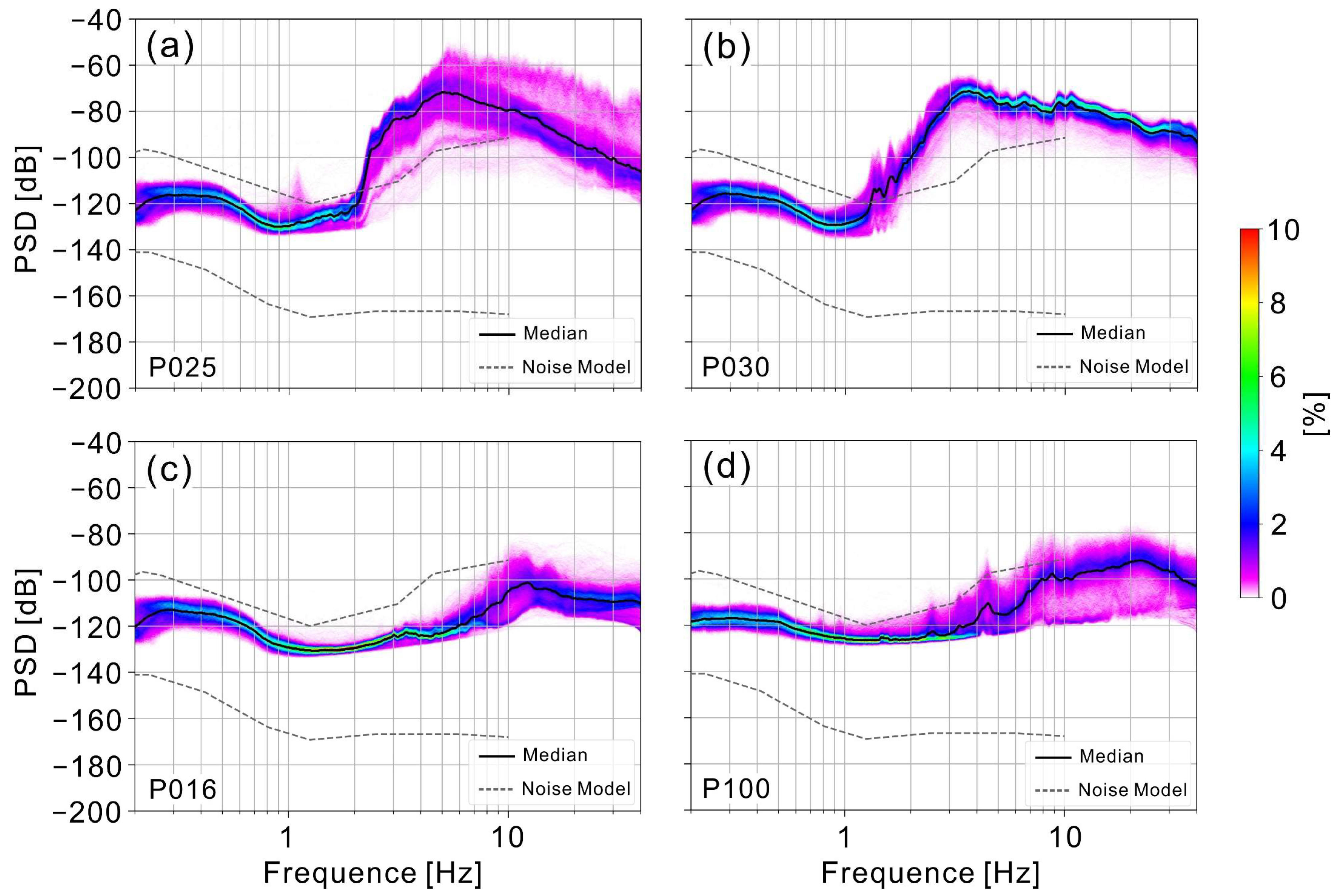
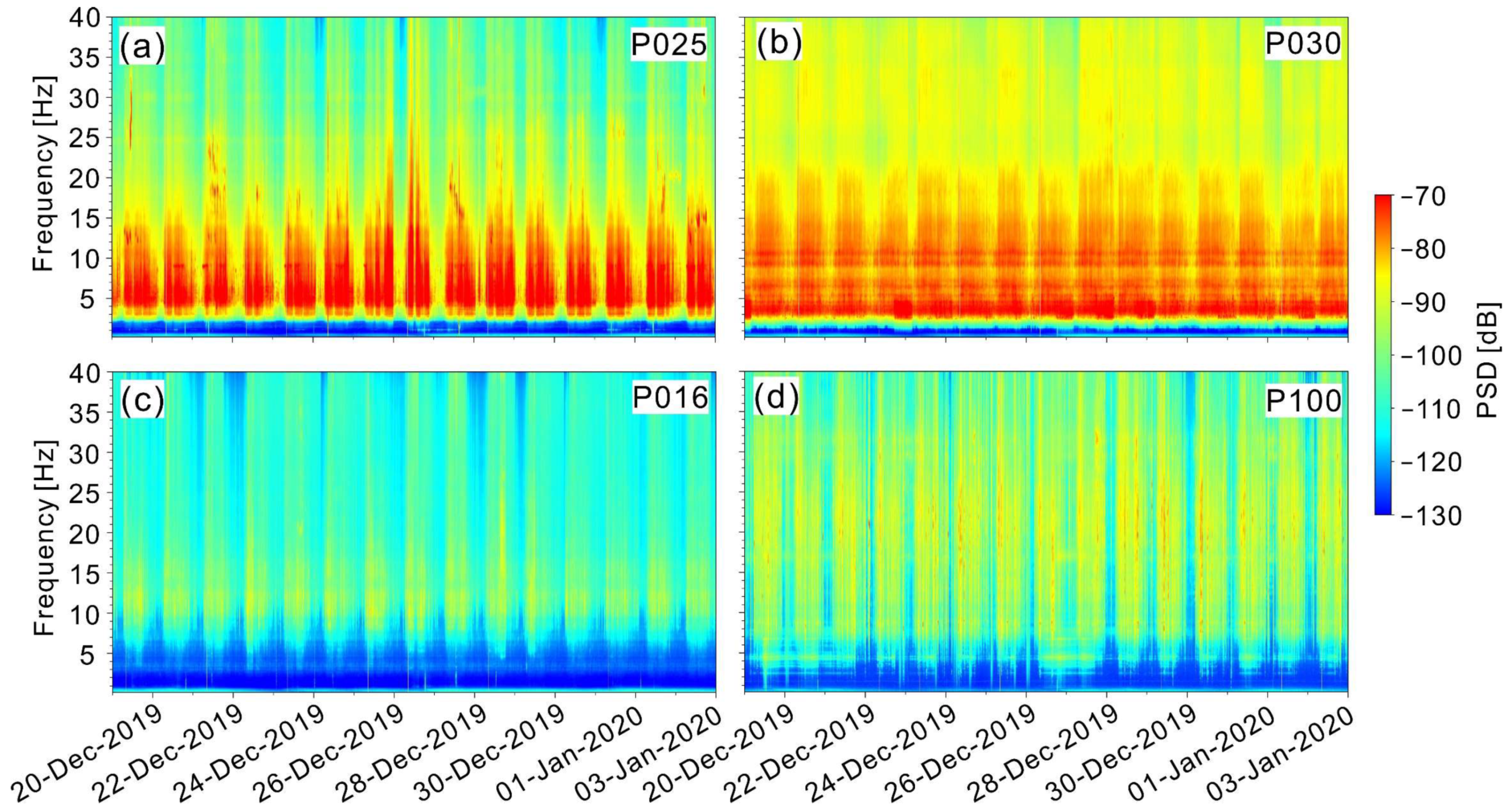
3.1. Characteristics of Cultural Seismic Noise in the GBA

Previous studies have shown that seismic noise in different frequency bands has different sources and generation mechanisms [16,57]. Seismic noise with a frequency greater than 1 Hz is primarily produced by human activity. These activities generate vibrational energy that is coupled to the Earth and propagates through high-frequency surface waves, attenuating within a few kilometers of the noise source [58,59]. Therefore, based on the frequency characteristics of cultural seismic noise, we focused on seismic noise greater than 1 Hz.
We calculated the PSD-PDFs and spectrograms for the vertical components at each station (Figure 2, Figure 3 and Figure 4). We analyzed seismic noise data from November 2019 to 24 January 2020 (before the COVID-19 pandemic outbreak), aiming to minimize the effects of the pandemic on human activities and learning about the characteristics of cultural seismic noise in the GBA before the pandemic. The impact of the COVID-19 pandemic on GBA is discussed in Section 4.2. In this study, we selected four representative stations located at different settings in the GBA (Figure 1). P025 and P030 were located in densely populated urban areas with abundant human activity. The PSDs of the vertical components at these stations exhibited a rapid increase at approximately 2 Hz and soon exceeded the high-noise model proposed by Peterson [55] as the frequency increased (Figure 2a,b). P016 and P100 were located in sparsely populated rural areas with limited human activity. The PSDs of these stations were basically between the high-noise model and low-noise model (Figure 2c,d). The PDF diagrams of all the stations show a clear “separation” or “dispersion” phenomenon in the frequency band above 2 Hz, which corresponds to the day and night variations in human activities [59]. This result indicates that all stations have recorded different levels of cultural seismic noise.
To compare the noise levels among different stations, we calculated the median PSD of each station, which represented the noise levels at different frequencies (black solid line in Figure 2). This approach has been widely used in various regions [42,59,60]. Figure 3 shows the median PSDs of the vertical components for all stations. The median PSDs of 49 stations significantly exceeded the high-noise model proposed by Peterson [55]. The peak frequency of cultural seismic noise was mainly concentrated between 2 and 20 Hz (Figure 3, blue circles). Furthermore, Figure 3 indicates that the level of cultural seismic noise in the GBA ranges between −160 dB and −60 dB, with a change of up to 100 dB at different stations. The red solid line in Figure 3 represents the average curve of the median PSDs for all stations, revealing that cultural seismic noise begins to increase rapidly at frequencies greater than 2 Hz, and the peak frequency is approximately 14 Hz.
By analyzing the spectrogram of each station, we identified the dominant frequency bands of cultural seismic noise in the GBA (Figure 4). Previous studies have demonstrated that cultural seismic noise typically exhibits a diurnal pattern corresponding to people’s daily routines, with greater intensity during the day than at night and weaker intensity on weekends than on weekdays [14,61,62]. Consequently, we examined the spectrograms for each station based on this feature. For stations in urban areas, cultural seismic noise was primarily concentrated in the range of 2–20 Hz. Although seismic noise greater than 20 Hz exhibited a diurnal pattern, its intensity was relatively weak (Figure 4a,b). The stations in rural areas showed similar characteristics but with weaker intensities compared to the stations in urban areas (Figure 4c,d). Moreover, the peak frequencies of cultural seismic noise in the GBA, as shown in Figure 3, were mainly concentrated in the range of 2–20 Hz (Figure 3). Thus, we proposed that the 2–20 Hz range is the dominant frequency band for cultural seismic noise in the GBA. Next, we explored the relationship between cultural seismic noise and human activities in this frequency band.

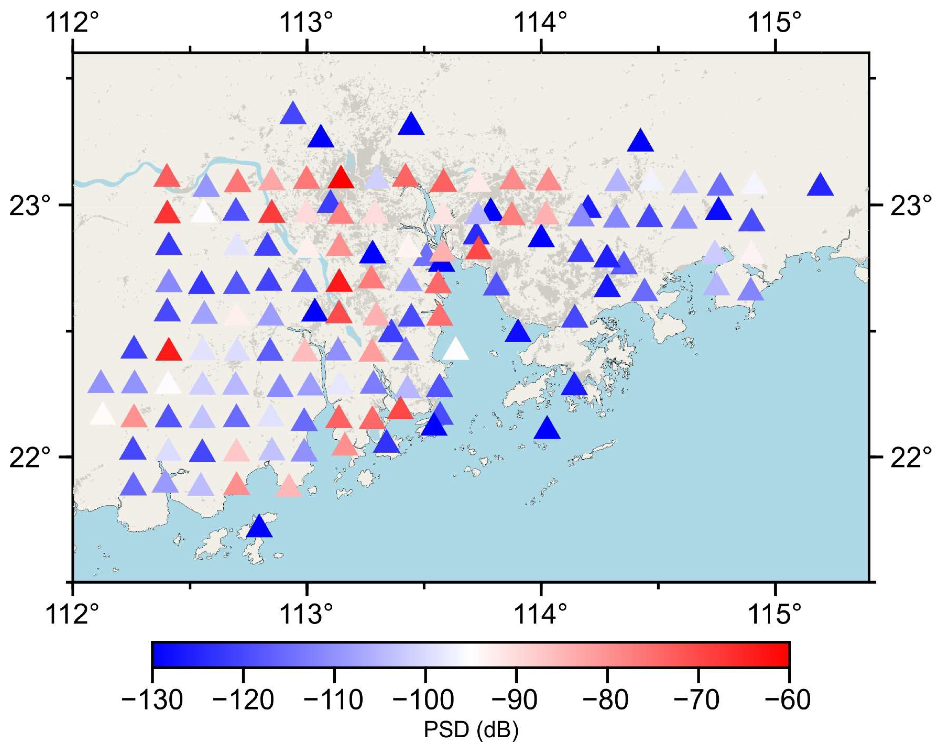
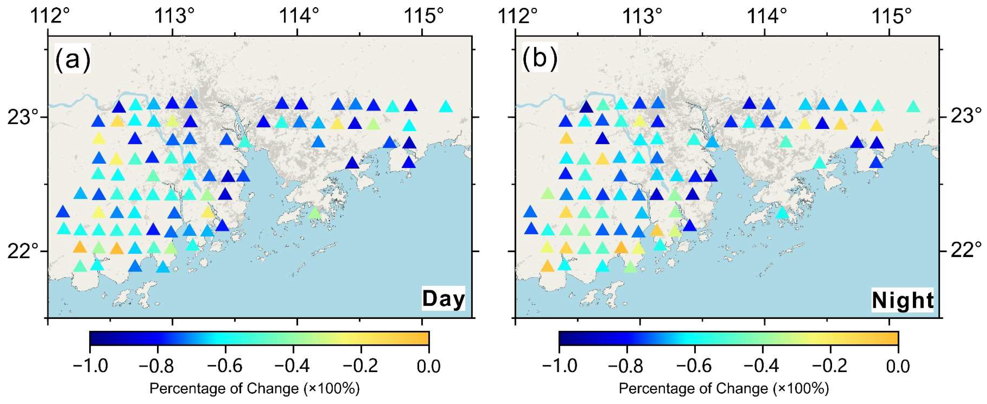
3.2. Spatial Distribution of Cultural Seismic Noise in the GBA

Previous studies have shown that cultural seismic noise levels are closely related to regional population density and economic development [44,63,64]. Consequently, we analyzed the correlation between cultural seismic noise and population density [65] as well as gross domestic product (GDP) [66,67] in the GBA (Figure 5 and Figure 6). Figure 6a,b illustrate the spatial distribution of population density and GDP in the GBA, respectively. Overall, population density and GDP had similar spatial distributions, both exhibiting higher values in Guangzhou, Shenzhen, Foshan, and Hong Kong (Figure 1 and Figure 6a,b). As the cultural seismic noise in the GBA was concentrated at 2–20 Hz, we calculated the average noise level in this band based on the median PSD of each station. Figure 5 shows the spatial distribution of cultural seismic noise in the GBA. High noise levels were mainly concentrated in Guangzhou, Foshan, Dongguan, and Zhongshan, which corresponded to the distributions of population density and GDP. However, Shenzhen and Hong Kong exhibited different features due to the limited number of stations (Figure 1, Figure 5 and Figure 6a,b). On average, cultural seismic noise in urban areas was approximately 30 dB higher than that in rural areas (Figure 5), indicating the impact of population and economy on local cultural seismic noise. To further investigate, we calculated the average population density and GDP within a 10 km radius of each station. The correlation analysis revealed a correlation coefficient of 0.32 between cultural seismic noise and population density and a correlation coefficient of 0.27 between cultural seismic noise and GDP. The linear relationships between these parameters are shown in Figure 6c,d.

4. Discussion

4.1. Daily Human Activity
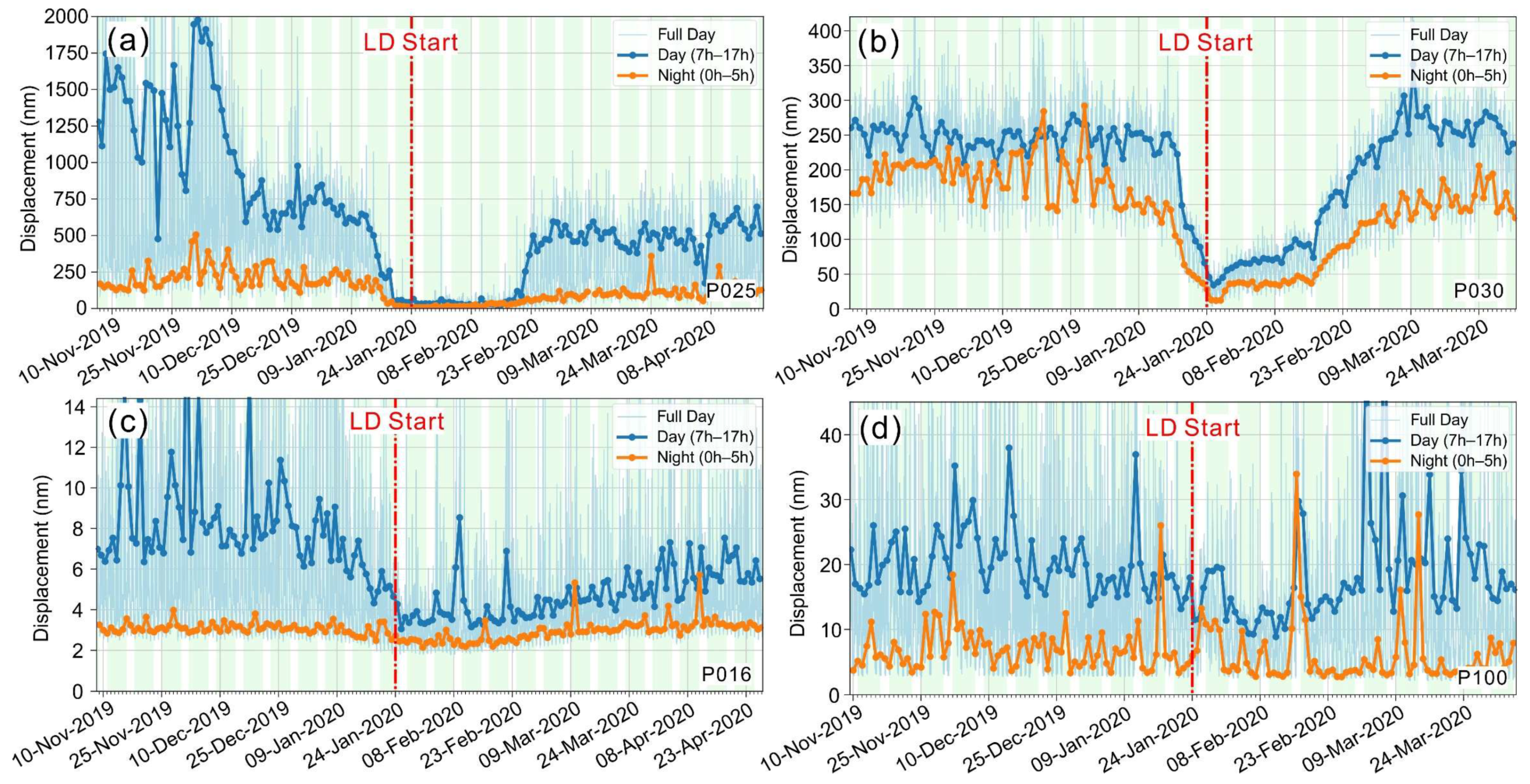
A multitude of human activities occur at or near the Earth’s surface at various times and locations. Seismometers in urban environments record daily human activity as near-continuous signals. These intricate signals are generally stronger during the day than at night, less intense on weekends than on weekdays, and more pronounced in urban areas than in rural areas [13,61,62]. Moreover, human activities can be influenced by inclement weather or traditional festivals [64,68,69]. As mentioned previously, the dominant frequency of cultural seismic noise ranges from 2 to 20 Hz in the GBA. Consequently, in our subsequent analysis, we specifically focused on seismic noise within this frequency band to explore the characteristics of daily human activity in the GBA.

4.1.1. Day/Night

Diurnal variation is the most significant feature of human activity [61,62,63]. Owing to regional differences in human activity, the daily cultural seismic noise exhibited distinct patterns at each station. We can learn about the work and rest schedules of local residents by analyzing the daily fluctuations in cultural seismic noise [14,44,62]. In this study, we calculated the daily variation of cultural seismic noise at each station in the GBA. Figure 7 shows two representative stations. Generally, cultural seismic noise reached its minimum between 0 a.m. and 5 a.m., then rapidly increased, peaking between 7 a.m. and 10 a.m. It temporarily decreased between 11 a.m. and 2 p.m. and later swiftly recovered and persisted until approximately 5 p.m. local time. Subsequently, the cultural seismic noise rapidly declined until midnight (Figure 7a,c). In addition, some urban environmental stations maintained relatively high noise levels during the night, which correlated with the city’s nightlife (Figure 7a). Interestingly, a few stations, such as P003, exhibited higher noise levels at night. We suggested that this phenomenon might be attributable to the traffic conditions near the station. There is a highway located approximately 80 m northwest of P003. We surmised that the traffic flow on this highway might be greater at night than during the day, which could potentially explain the stronger nighttime noise level at P003 (Figure 8). To comprehend the diurnal variation characteristics of human activity in the GBA, we calculated the daytime (7 a.m.–5 p.m.) and nighttime (0 a.m.–5 a.m.) noise levels at each station. The results indicated that 95% of the stations in the GBA exhibited day and night variations in noise levels associated with human activities (Figure 9a). The average nighttime noise level in the GBA decreased by 40.4% compared to the daytime noise level, with stations in urban areas experiencing significant changes (Figure 9a).

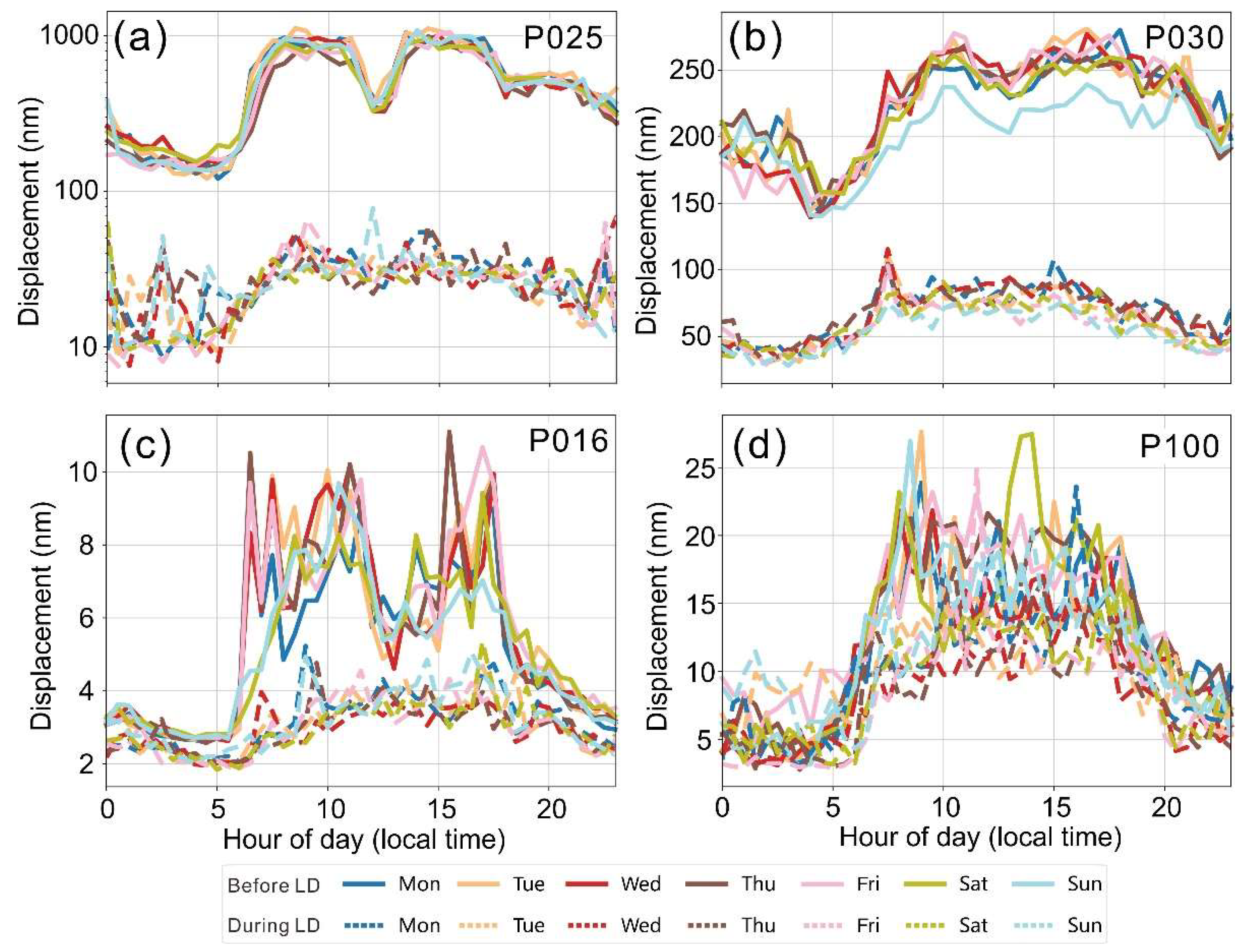
4.1.2. Weekdays/Weekends

Another notable aspect of human activity is the distinction between weekdays and weekends [14,63,70]. In contrast to the obvious variation in day and night, the difference between weekdays and weekends’ cultural seismic noise in the GBA was relatively minimal and not universally observed across all stations (Figure 7 and Figure 9b). Generally, the noise levels on weekdays were higher than those on weekends, and the main differences occurred during the daytime hours (Figure 7a). However, the noise levels in rural areas remained virtually identical on weekdays and weekends (Figure 7c). To examine the variation in cultural seismic noise in the GBA between weekdays and weekends, we calculated the average noise level for both weekdays and weekends during the daytime hours (7 a.m.–5 p.m.) at each station. On average, the noise level in the GBA was approximately 1.8% lower during the weekends. Furthermore, the stations with decreased seismic noise were predominantly located in urban areas (Figure 9b), highlighting the differences in living patterns between urban and rural populations in the GBA.

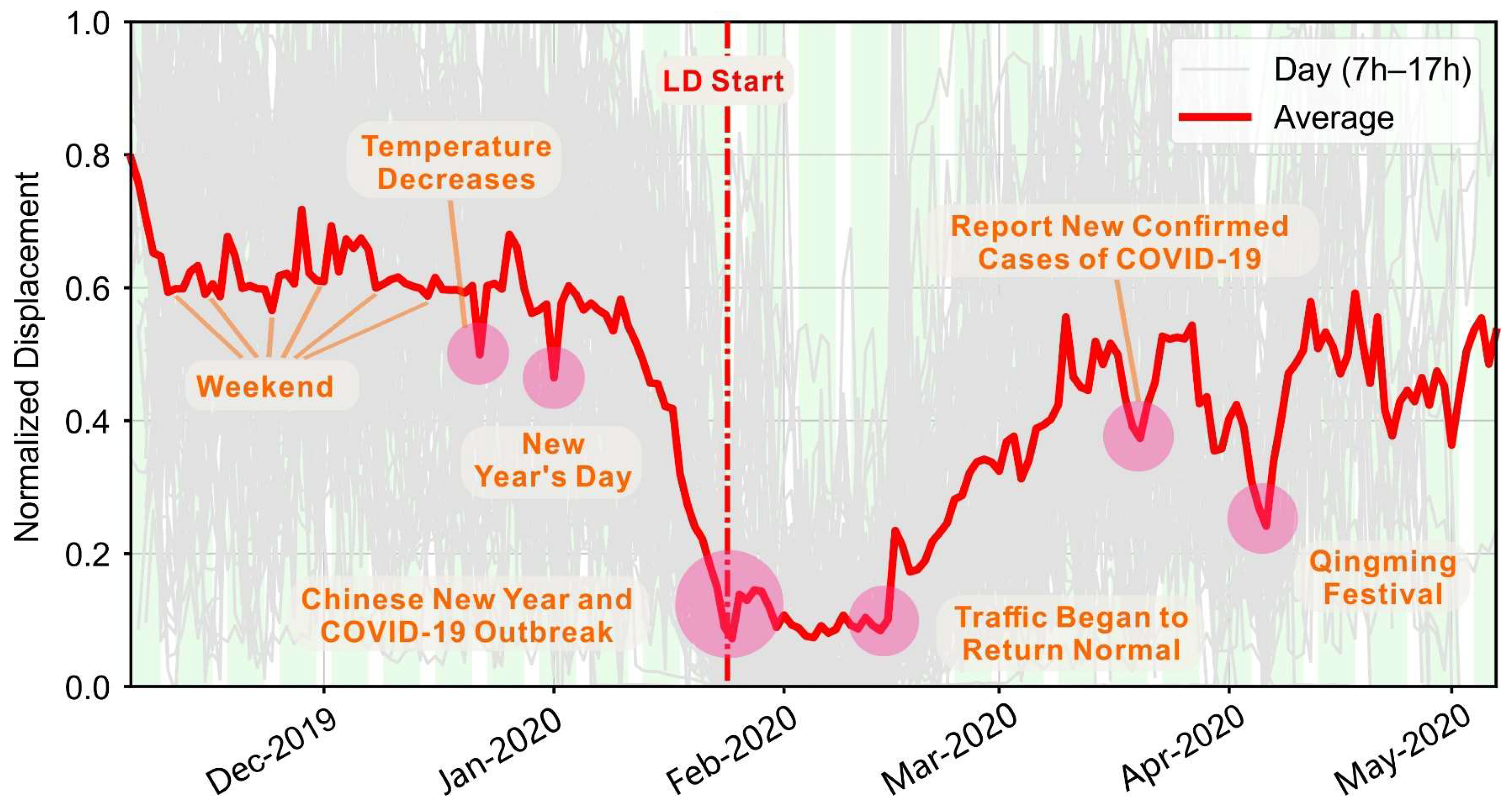
4.1.3. Traditional Festival

Previous studies have shown that cultural seismic noise changes significantly during traditional festivals such as the Chinese Spring Festival [44,64], Christmas [13,69], and others. In our dataset, 120 stations recorded cultural seismic noise during the New Year’s Days, a three-day holiday for Chinese citizens. Due to factory closures and school vacations, cultural seismic noise levels on New Year’s Day were considerably lower than usual (Figure 7b and Figure 10). To investigate the variations in cultural seismic noise within the GBA on New Year’s Day, we computed the average noise levels at each station during this period. The results showed that 77% of the stations experienced a reduction in noise levels (Figure 9c). The average noise level in the GBA decreased by approximately 8.1% on New Year’s Day, indicating a more substantial reduction and broader impact than those observed on weekends (Figure 9b,c).

4.1.4. Temperature Drop

Daily weather changes also affect human activity [68]. In our dataset, two significant decreases in cultural seismic noise occurred before the COVID-19 pandemic outbreak (Figure 10). We believed that one decrease resulted from the impact of New Year’s Day, based on the timing of its occurrence. However, what caused the other drop in cultural seismic noise before New Year’s Day? Upon further investigation, we inferred that weather conditions were the most likely influencing factors. According to a report from the Guangdong Provincial Meteorological Bureau, the average temperature across the entire province dropped by 6–8 °C from 18 to 23 December in 2019 due to cold air and local rainfall (Figure 7b,d). This sudden temperature drop reduced people’s willingness to travel, leading to changes in the cultural seismic noise recorded by the stations. To assess the impact of this temperature drop on cultural seismic noise in the GBA, we calculated the average noise level at each station during this period. However, as this coincided with a weekend, we compared the results with the average noise levels on other weekends to exclude the influence of weekends on cultural seismic noise. The results revealed that 64% of stations experienced a reduction in cultural seismic noise (Figure 9d). The average noise level in the GBA decreased by approximately 5% due to the temperature drop. Interestingly, the affected stations were primarily located in rural areas, while the urban areas remained largely unaffected (Figure 9d). The two representative stations, as depicted in Figure 7, exhibited distinct characteristics. P030, which is situated in an urban area, primarily displayed differences between weekdays and weekends, with no impact from weather changes on its recorded cultural seismic noise. In contrast, P100, which is located in a rural area, was more prone to changes induced by weather (Figure 7b,d).

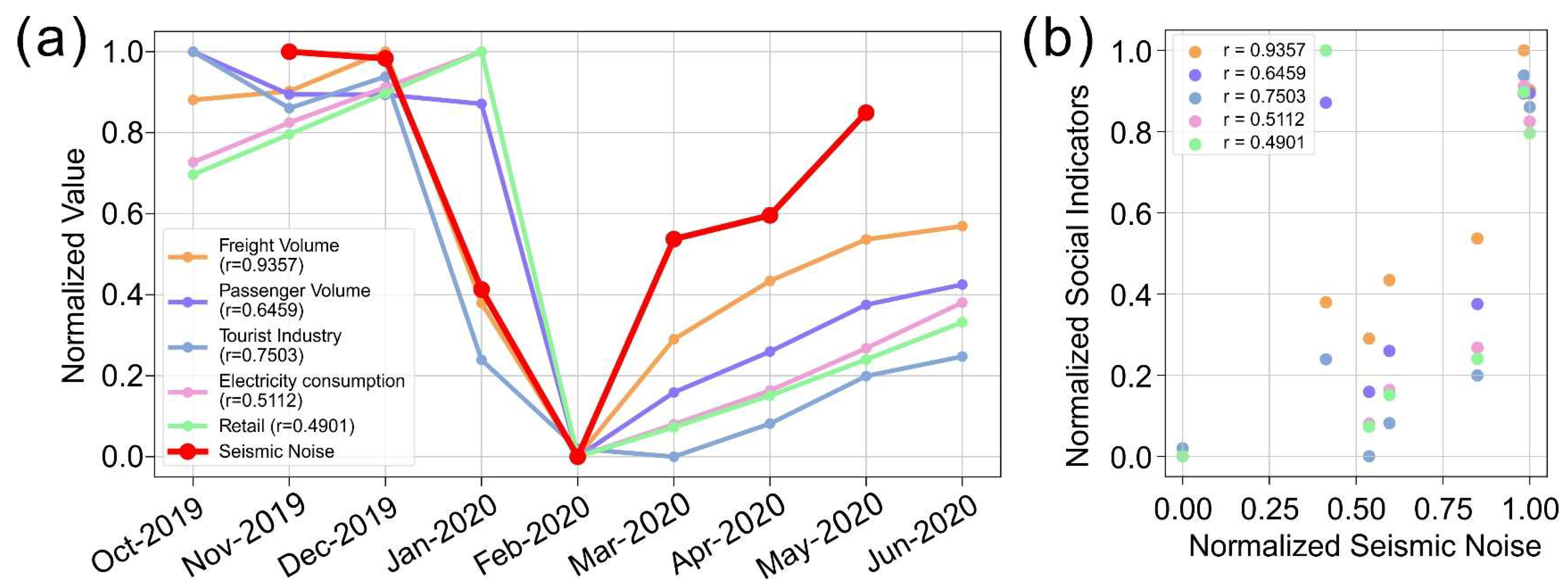
4.2. Impact of COVID-19 Pandemic on GBA

The World Health Organization declared the coronavirus disease 2019 (COVID-19) outbreak a global health emergency in January 2020 and a pandemic in March 2020 [71]. After the COVID-19 pandemic outbreak, China firstly implemented emergency lockdown measures and restricted all non-essential human activities. Schools, shopping malls, factories, and other public places were successively closed to mitigate the spread of the virus [72]. Subsequently, other countries also implemented lockdown measures [13,41,73]. Although the COVID-19 pandemic has been brought under control, the lockdown measures have significantly affected people’s daily lives, industrial production, and other human activities. During the COVID-19 pandemic, cultural seismic noise studies worldwide have revealed a significant reduction in global high-frequency seismic noise owing to the decrease in human activity [13,42,43]. Since the first case was reported in Guangdong Province on 19 January 2020, the number of infected individuals in Guangdong has rapidly increased. On 24 January, Guangdong Province initiated a Level 1 response to this major public health event by implementing lockdown measures and restricting all non-essential human activities. Subsequently, national and local governments adopted dynamic measures depending on the number of new cases. On 24 February 2020, Guangdong Province adjusted the response level to Level 2 and lifted the lockdown measures. To investigate the impact of the COVID-19 pandemic on human activity in the GBA, we examined the spatial and temporal characteristics of cultural seismic noise in the GBA during this period.
In our dataset, 88 stations recorded cultural seismic noise during the COVID-19 pandemic. In this study, we assessed the impact of the lockdown measures on cultural seismic noise during the pandemic. The results show that 79 stations experienced a significant decrease in cultural seismic noise during the COVID-19 pandemic (Figure 11). Cultural seismic noise in the GBA began to decline around 17 January 2020, coinciding with the approach of the Spring Festival, during which factories, schools, and other establishments successively closed (Figure 11). Cultural seismic noise reached its minimum level around 24 January (Spring Festival), the same day when Guangdong Province initiated the lockdown measures to restrict all non-essential social activities. Subsequently, most stations underwent a “quiet period” lasting approximately 24 days, until about February 17 when cultural seismic noise began to gradually recover (Figure 11).
Figure 12 shows the variation characteristics of cultural seismic noise at four typical stations in different environments. For stations located in urban areas, such as P025 and P030, a significant reduction in cultural seismic noise was observed during the lockdown period. These stations experienced a “quiet period” of approximately 24 days until February 17, 2020, when the cultural seismic noise began to rise rapidly and then returned to the pre-lockdown noise levels in a short time (Figure 12a,b). During the lockdown, the daytime cultural seismic noise decreased by 94% in P025 and 65% in P030, whereas the nighttime cultural seismic noise decreased by 91% in P025 and 78% in P030. However, for the stations in rural areas, such as P016 and P100, the reduction in cultural seismic noise was less or remained relatively stable during the lockdown (Figure 12c,d). At station P016, the cultural seismic noise decreased by 54% and 19% during the daytime and nighttime, respectively, and gradually recovered after the lockdown ended (Figure 12c). At station P100, the cultural seismic noise remained relatively stable before and after the lockdown, decreasing by 20% and 10% during the daytime and nighttime, respectively (Figure 12d). Overall, during the lockdown period, the daytime and nighttime cultural seismic noise in the GBA average decreased by 61% and 57%, respectively, and the stations with larger decreases were basically located in urban areas (Figure 13). These results suggest that urban areas have been more severely affected by the pandemic than rural areas.
After the outbreak of the COVID-19 pandemic, the pattern of human activity in the GBA changed significantly owing to the implementation of the lockdown measures. Figure 14 shows the variation in cultural seismic noise throughout the day at four typical stations in different environments before and after the lockdown. Firstly, before the lockdown, some stations exhibited higher cultural seismic noise levels on weekdays than on weekends. However, after the lockdown, this difference diminished, as observed at station P030 (Figure 14b). Secondly, during the lockdown period, some stations no longer displayed a slight decrease in cultural seismic noise during lunchtime (11 a.m.–2 p.m.), such as stations P025 and P016 (Figure 14a,c). Finally, the lockdown measures changed people’s night lives. For example, before the lockdown, the nighttime cultural seismic noise at station P030 remained at a high level and lasted until midnight, but this phenomenon disappeared after the lockdown (Figure 14b). Notably, not all stations experienced changes in cultural seismic noise after the lockdown, such as some stations in rural areas where the cultural seismic noise level and pattern remained essentially the same before and after the lockdown (Figure 14d). Thus, these results suggest that the cultural seismic noise recorded by stations can reflect changes in people’s lifestyles during the COVID-19 pandemic.
Here, we aimed to analyze the factors that contributed to the changes in cultural seismic noise observed in the GBA during different periods (Figure 15). As mentioned above, the variation in cultural seismic noise between weekdays and weekends was small before the COVID-19 pandemic outbreak, and two significant decreases in cultural seismic noise were observed owing to the temperature drop and New Year’s Day. As the Spring Festival approached, the overall cultural seismic noise in the GBA began to decline rapidly as factories, schools, and other establishments closed sequentially, and then reached its lowest point on 24 January 2020. The COVID-19 pandemic outbreak and subsequent lockdown measures coincided with the Spring Festival. During the lockdown period, all non-essential human activities were restricted in the GBA to reduce the spread of the virus. As a result, most areas experienced a “quiet period” of approximately 24 days. Interestingly, the recovery of cultural seismic noise began on 17 February 2020, even before the lockdown measures were lifted. Upon further investigation, we discovered that the Chinese government implemented a national toll road-free access policy on 17 February 2020, which led to a gradual return of traffic flow and subsequent recovery of cultural seismic noise in the GBA. This finding suggests that the cultural seismic noise recorded by the stations mainly originated from vehicles. By mid-March 2020, the cultural seismic noise in the GBA returned to near pre-pandemic levels, followed by several significant decreases. We speculated that the first decline in cultural seismic noise was due to the sudden increase in the number of people infected with the virus, leading to a reduction in people’s activities outside for health. The second significant decline occurred during the Qingming Festival, a traditional Chinese festival during which Chinese people have a three-day holiday and memorialize their ancestors. During this period, cultural seismic noise dropped approximately twice as much as on New Year’s Day before the COVID-19 pandemic outbreak. We inferred that the main reason for this phenomenon was that the Chinese government called on the public to reduce travel arrangements and avoid the movement of people during holidays influenced by the COVID-19 pandemic. As a result, it enhanced the decline in cultural seismic noise during the festival. Based on the characteristics of cultural seismic noise changes before and after the COVID-19 pandemic in the GBA, it is evident that monitoring and analyzing cultural seismic noise over time can provide valuable insights into human activity during different periods.
Furthermore, we compared the variations in cultural seismic noise with other social statistical data from the GBA (Figure 16). Transportation, industrial production, tourism, and retail trade in the GBA have been greatly affected by the COVID-19 pandemic. As expected, there were strong correlations between cultural seismic noise and these social statistical data, and all exhibited a considerable decline during the pandemic. Among these, freight volume shows the highest correlation coefficient of 0.9357 (Figure 16). Notably, significant differences were observed among the various data types. For instance, cultural seismic noise rebounded swiftly following the lifting of the lockdown, and noise levels in May 2020 approached those before the COVID-19 pandemic outbreak. Conversely, the social statistical data exhibited a more gradual recovery, and in June 2020, they had not yet returned to their pre-pandemic levels (Figure 16a).

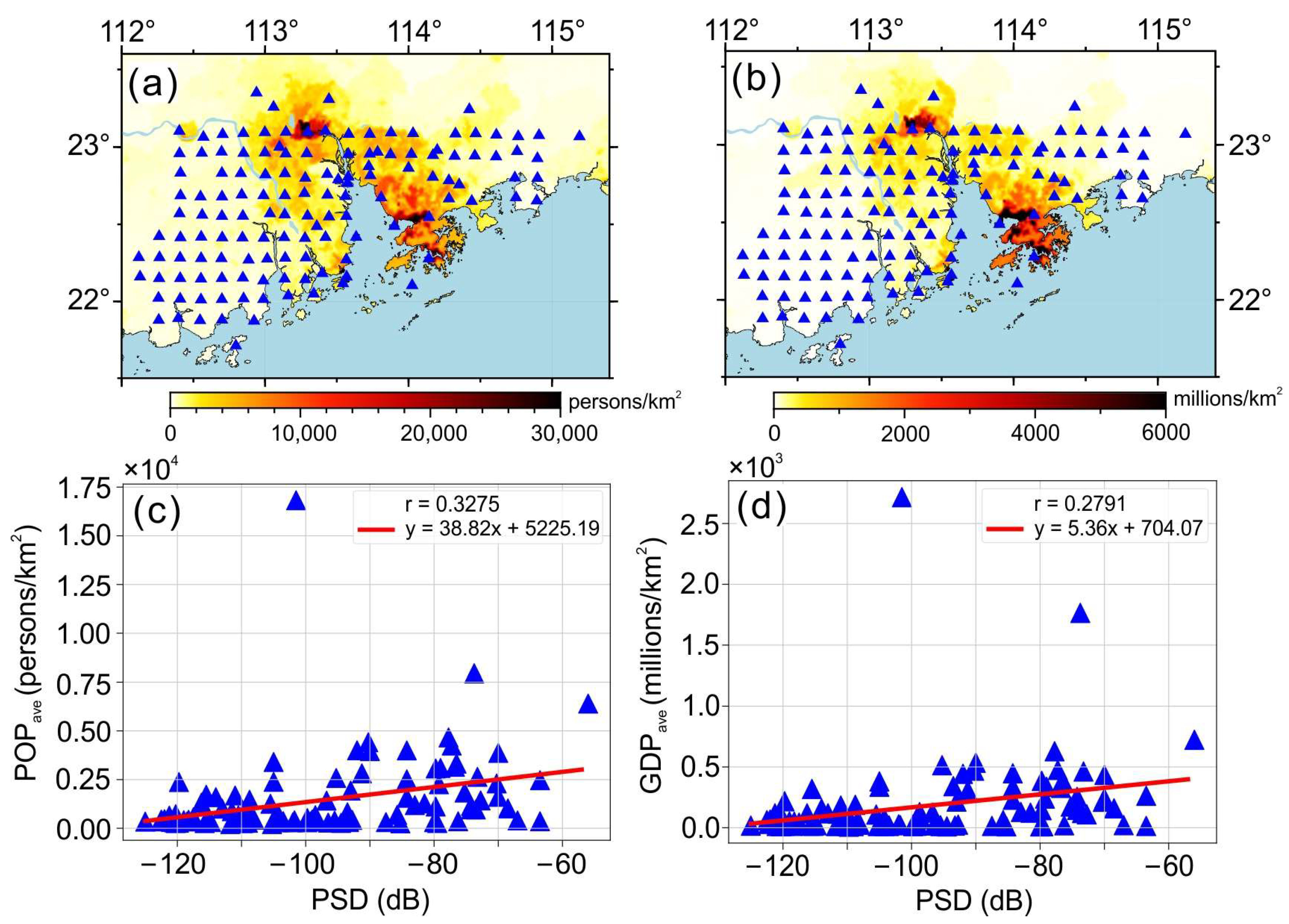
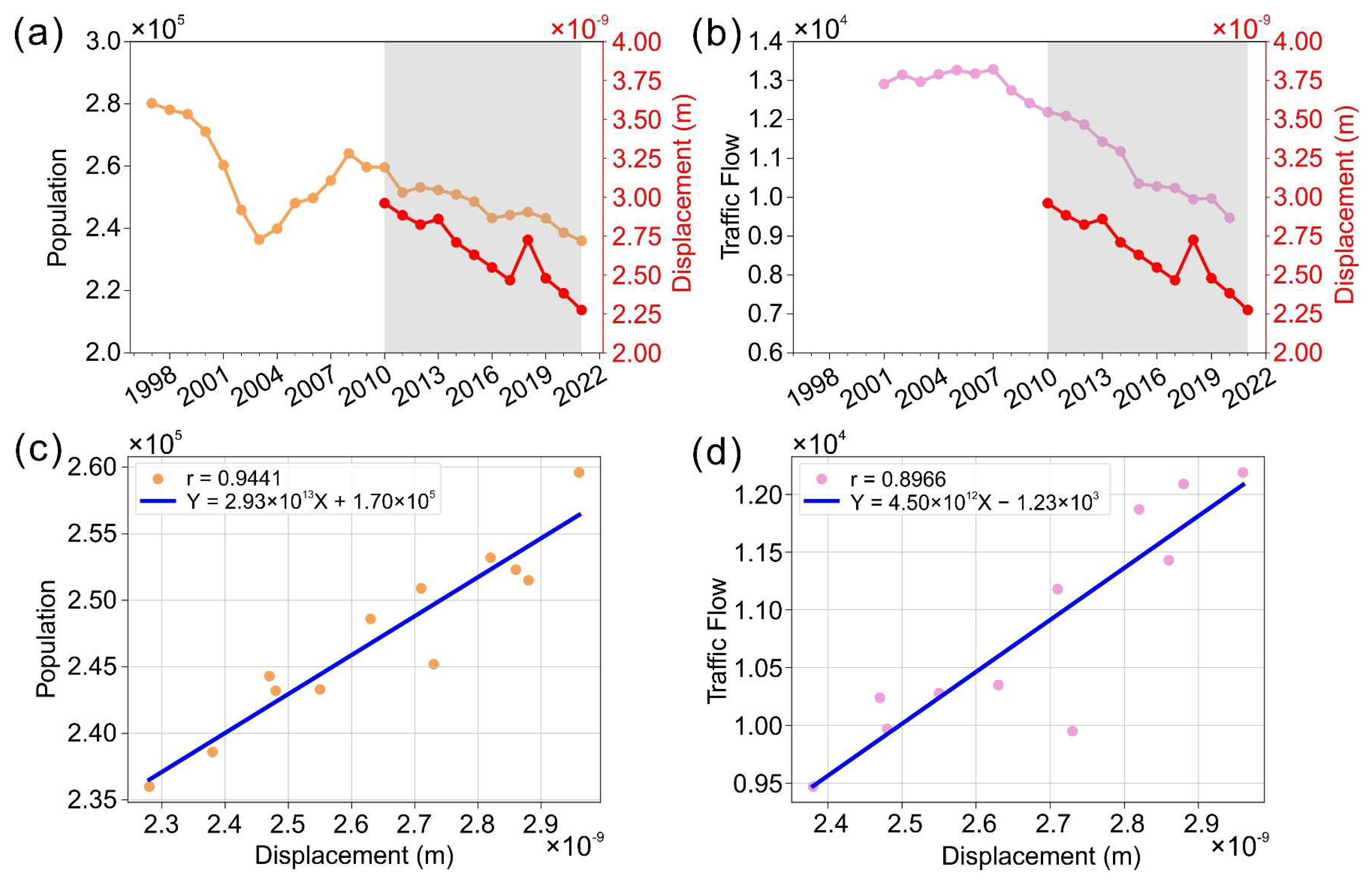
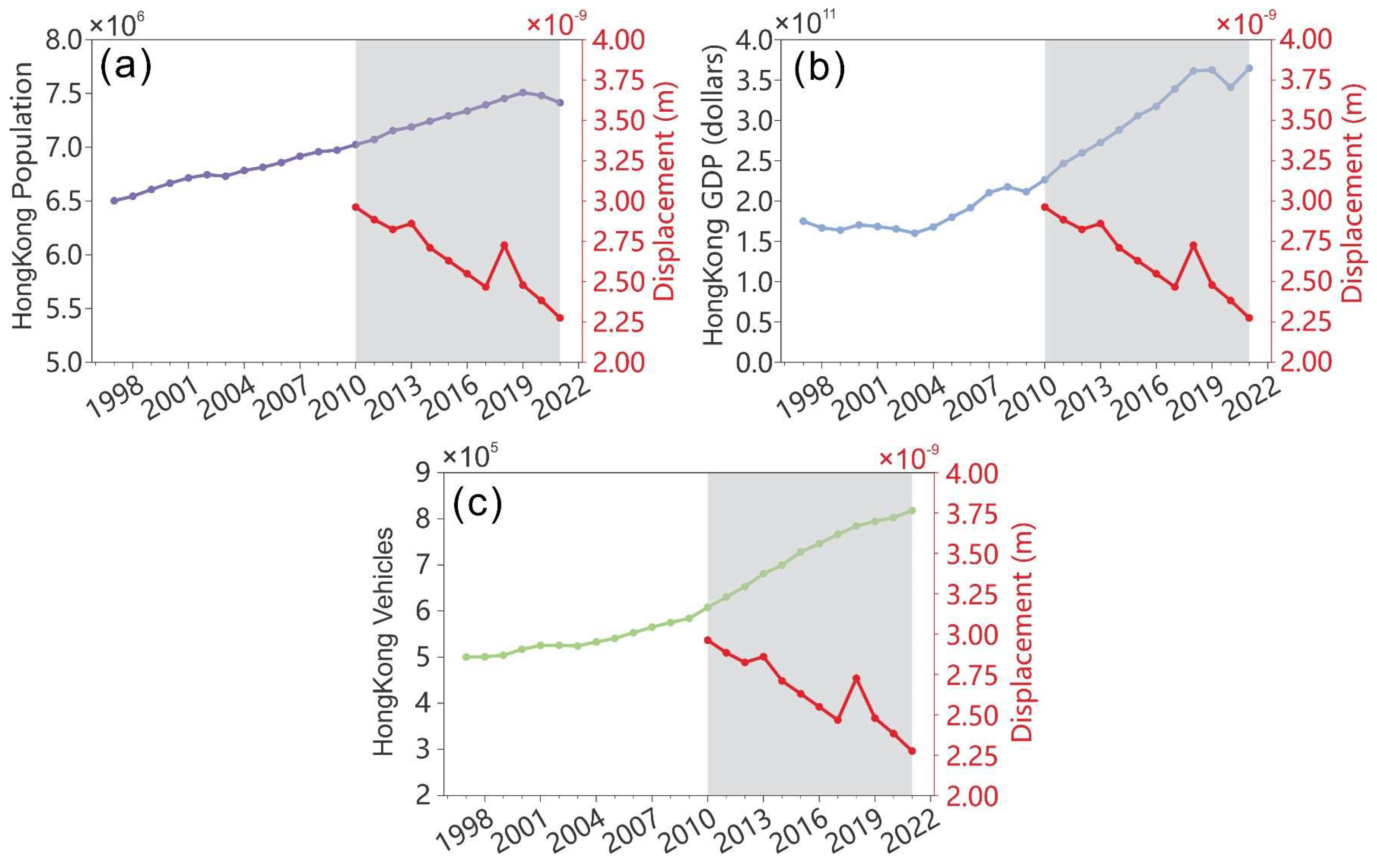
4.3. Human Society Development

Over the past few decades, the global economy and population have experienced continuous growth, and cultural seismic noise has also changed. In this study, we used 12-year-long seismic data from the Hong Kong seismic station (HKPS) to analyze the relationship between long-term cultural seismic noise changes and social development in Hong Kong. The HKPS seismic station is located in the Central and Western District of Hong Kong, which has a population of approximately 240,000 people and is among the first areas to be developed in Hong Kong. Here, we analyzed the daytime (7 a.m.–5 p.m.) cultural seismic noise between 2 and 20 Hz at this station. The results showed a decreasing trend in cultural seismic noise over the 12 years, with a 23% decrease compared to the noise levels measured in 2010 (Figure 17a,b). Concurrently, when comparing the changes in population and traffic flow in Hong Kong’s Central and Western District from 2010 to 2021, it was observed that the local population declined by 9%, and road traffic declined by 22.3% over the past 12 years (Figure 17a,b). Correlation analysis revealed that the correlation coefficients between cultural seismic noise and population, as well as road traffic in the Central and Western District, were 0.9441 and 0.8966, respectively, and the linear relationships were depicted in the graphs (Figure 17d,c). Interestingly, when comparing the changes in population, GDP, and vehicles for the entire Hong Kong region, the results were the opposite. Over the past 12 years, the population, GDP, and vehicles in Hong Kong increased by 5.5%, 61.1%, and 34.6%, respectively (Figure 18). These results show a completely different trend from the variation in cultural seismic noise, indicating that long-term analysis of cultural seismic noise can be another potential way of understanding local social development.

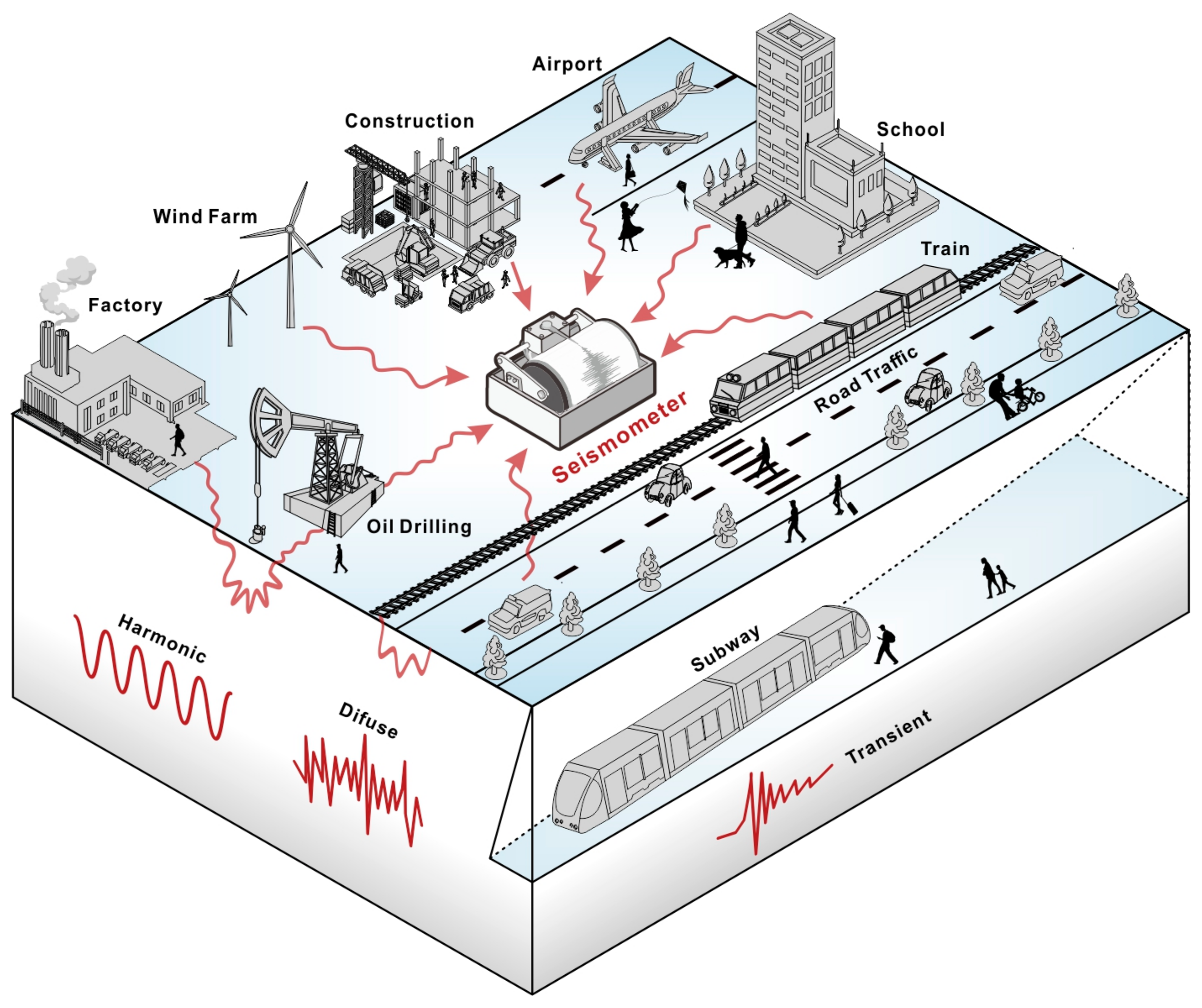
4.4. Sensing Human Activity by Seismometer

Our planet vibrates constantly, sometimes with remarkable intensity but more often with imperceptible intensity. Conventional seismology typically relies on rare large earthquakes to decipher vibration sources and path effects. However, human activities on the Earth’s surface also generate seismic waves, which can be detected by seismometers at great distances. Whether the source is transient (recreational; individual cars, trains, or airplanes), harmonic (wind turbines, machinery), or diffuse (railroads, highways) (Figure 19), seismometers can record vibrations in everything [74]. Everyday human activity is recorded as a near-continuous signal, especially on seismometers in urban environments. These complicated signals are the superposition of a wide variety of activities happening at different times and places at or near Earth’s surface (Figure 19) [13]. By analyzing these signals using seismological techniques, we can learn about the spatial and temporal characteristics of human activity. However, ambient seismic noise recorded by seismometers currently offers only an indirect and coarse measure of human activity intensity due to the spatial variation and temporal overlap of multiple noise sources. Therefore, many seismologists are currently committed to studying the signal characteristics of different human and natural activities in order to achieve specific target monitoring [15,75,76]. Although there are currently some limitations to this tool, ambient seismic noise monitoring has several notable advantages. For example, seismometers are relatively easy to install and maintain, and a mature system for real-time data transmission already exists. Furthermore, seismic data can be collected and utilized with minimal potential privacy concerns and without being affected by weather conditions. Moreover, with the development of fiber-optic distributed acoustic sensing technology, numerous communication fibers distributed underground in cities will likely replace seismometers for collecting ambient seismic noise data. These advantages pave the way for the systematic utilization of seismic sensors as tools for monitoring human activity in urban areas.

5. Conclusions

In this study, we investigated the relationship between human activity and ambient seismic noise using continuous waveform data recorded by 138 seismometers deployed in the GBA. Our results indicate that cultural seismic noise generated by human activity in the GBA is mainly concentrated in the range of 2–20 Hz. The spatial distribution of cultural seismic noise is strongly correlated with population and economy, which is characterized by higher noise levels in densely populated areas.
Through the analysis of cultural seismic noise during different periods, we successively studied the effects of daily human activity, the COVID-19 pandemic, and long-term social development on cultural seismic noise in the GBA. Research on cultural seismic noise before the COVID-19 pandemic outbreak demonstrated that monitoring cultural seismic noise could reveal the daily pattern of human activity. Both the diurnal variation in human activity and the distinction between weekdays and weekends were well represented in cultural seismic noise. Notably, we observed the spatial and temporal effects of New Year’s Day and a temperature drop on human activities.
As expected, cultural seismic noise in the GBA significantly decreased during the COVID-19 pandemic. The daytime and nighttime cultural seismic noise decreased by 61% and 57%, respectively. The stations with larger decreases were predominantly concentrated in urban areas, indicating that these areas were more severely affected by the pandemic. Concurrently, people’s daily routines were changed due to the pandemic’s impact, which was also evident in cultural seismic noise. By examining the variations in cultural seismic noise in the GBA before and after the pandemic outbreak, we discovered that abnormal fluctuations corresponded well with the large-scale human activity changes caused by holidays, national policies, and pandemic conditions. Furthermore, a strong correlation is found when comparing cultural seismic noise with various social statistical data in the GBA. The analysis of cultural seismic noise during the pandemic indicates that monitoring cultural seismic noise can provide valuable insights into human activity and assess the spatial and temporal impact of a specific event on human activity.
Moreover, the analysis of 12-year-long cultural seismic noise recorded by the HKPS revealed a close relationship between long-term changes in cultural seismic noise and local social development. This finding suggests that long-term changes in cultural seismic noise can serve as potential indicators of local social development.
In conclusion, effective monitoring of human activities is essential for social stability and urban development. Our study highlights that ambient seismic noise contains rich information about human activities and provides a good research case for the systematic use of seismic sensors as a tool for monitoring human activities in urban areas.

Author Contributions

Conceptualization, S.X.; Data curation, S.X.; Formal analysis, L.C. and S.X.; Funding acquisition, S.X.; Investigation, S.X.; Methodology, L.C. and S.X.; Project administration, S.X.; Software, L.C.; Supervision, S.X.; Validation, S.X.; Writing, original draft, L.C. and S.X.; Writing, review and editing, L.C. and S.X. All authors have read and agreed to the published version of the manuscript.

Funding

This research is funded by the National Key Research and Development Program of China, (Grant No. 2022YFC3102200) and the National Natural Science Foundation of China (Grant No. 42076071).

Data Availability Statement

Not applicable.

Acknowledgments

The authors are grateful to the MAGMAN research team members for their participating the field work and data acquisition, and the Guangdong Earthquake Agency (http://www.gddzj.gov.cn, accessed on 6 January 2022.) and Incorporated Research Institutions for Seismology (IRIS; https://www.iris.edu, accessed on 22 October 2022.) for providing partial waveform data. The population data and Gross Domestic Product (GDP) data for Guangdong are from https://www.resdc.cn, accessed on 16 November 2022. Hong Kong’s population, traffic flow and GDP data are from https://www.censtatd.gov.hk, accessed on 3 May 2022. The social statistical data in the GBA are from https://www.stats.gd.gov.cn, accessed on 26 May 2022. The meteorological data are from http://gd.cma.gov.cn/, accessed on 13 April 2022. This work has benefited from open source initiatives such as Obspy [52] and GMT [77]. Data analysis has been carried out using the publicly available SeismoRMS code kindly distributed by Lecocq et al. [53]. We appreciate to the anonymous reviewers and the editors for their thorough examination of the manuscript and their valuable suggestions for improvement.

Conflicts of Interest

The authors declare no conflict of interest.

References

  1. UN-Habitat. World Cities Report 2020: The Value of Sustainable Urbanization; United Nations Human Settlements Programme: Nairobi, Kenya, 2020. [Google Scholar]
  2. Tenkanen, H.; Di Minin, E.; Heikinheimo, V.; Hausmann, A.; Herbst, M.; Kajala, L.; Toivonen, T. Instagram, Flickr, or Twitter: Assessing the usability of social media data for visitor monitoring in protected areas. Sci. Rep. 2017, 7, 17615. [Google Scholar] [CrossRef] [PubMed]
  3. Straczkiewicz, M.; James, P.; Onnela, J.-P. A systematic review of smartphone-based human activity recognition methods for health research. NPJ Digit. Med. 2021, 4, 148. [Google Scholar] [CrossRef] [PubMed]
  4. Shorfuzzaman, M.; Hossain, M.S.; Alhamid, M.F. Towards the sustainable development of smart cities through mass video surveillance: A response to the COVID-19 pandemic. Sustain. Cities Soc. 2021, 64, 102582. [Google Scholar] [CrossRef] [PubMed]
  5. Halder, B.; Bandyopadhyay, J.; Banik, P. Monitoring the effect of urban development on urban heat island based on remote sensing and geo-spatial approach in Kolkata and adjacent areas, India. Sustain. Cities Soc. 2021, 74, 103186. [Google Scholar] [CrossRef]
  6. Hu, T.; Wang, S.; She, B.; Zhang, M.; Huang, X.; Cui, Y.; Khuri, J.; Hu, Y.; Fu, X.; Wang, X.; et al. Human mobility data in the COVID-19 pandemic: Characteristics, applications, and challenges. Int. J. Digit. Earth 2021, 14, 1126–1147. [Google Scholar] [CrossRef]
  7. Liu, H.; Gamboa, H.; Schultz, T. Sensor-Based Human Activity and Behavior Research: Where Advanced Sensing and Recognition Technologies Meet. Sensors 2023, 23, 125. [Google Scholar] [CrossRef]
  8. Yadav, S.K.; Tiwari, K.; Pandey, H.M.; Akbar, S.A. A review of multimodal human activity recognition with special emphasis on classification, applications, challenges and future directions. Knowl. Based Syst. 2021, 223, 106970. [Google Scholar] [CrossRef]
  9. Liu, H.; Schultz, T. How Long Are Various Types of Daily Activities? Statistical Analysis of a Multimodal Wearable Sensor-based Human Activity Dataset. In Proceedings of the 15th International Joint Conference on Biomedical Engineering Systems and Technologies (BIOSTEC 2022)—HEALTHINF, Online, 9–11 February 2022; pp. 680–688. [Google Scholar] [CrossRef]
  10. Ronald, M.; Poulose, A.; Han, D.S. iSPLInception: An Inception-ResNet Deep Learning Architecture for Human Activity Recognition. IEEE Access 2021, 9, 68985–69001. [Google Scholar] [CrossRef]
  11. Liu, H.; Xue, T.; Schultz, T. On a Real Real-Time Wearable Human Activity Recognition System. In Proceedings of the 16th International Joint Conference on Biomedical Engineering Systems and Technologies—WHC, Lisbon, Portugal, 16–18 February 2023; pp. 711–720. [Google Scholar] [CrossRef]
  12. Jannat, M.K.A.; Islam, M.S.; Yang, S.H.; Liu, H. Efficient Wi-Fi-Based Human Activity Recognition Using Adaptive Antenna Elimination. IEEE Access 2023, 11, 105440–105454. [Google Scholar] [CrossRef]
  13. Lecocq, T.; Hicks, S.P.; Van Noten, K.; van Wijk, K.; Koelemeijer, P.; De Plaen, R.S.M.; Massin, F.; Hillers, G.; Anthony, R.E.; Apoloner, M.T.; et al. Global quieting of high-frequency seismic noise due to COVID-19 pandemic lockdown measures. Science 2020, 369, 1338–1343. [Google Scholar] [CrossRef]
  14. Díaz, J.; Ruiz, M.; Sanchez-Pastor, P.S.; Romero, P. Urban Seismology: On the origin of earth vibrations within a city. Sci. Rep. 2017, 7, 15296. [Google Scholar] [CrossRef]
  15. Riahi, N.; Gerstoft, P. The seismic traffic footprint: Tracking trains, aircraft, and cars seismically. Geophys. Res. Lett. 2015, 42, 2674–2681. [Google Scholar] [CrossRef]
  16. Díaz, J. On the origin of the signals observed across the seismic spectrum. Earth Sci. Rev. 2016, 161, 224–232. [Google Scholar] [CrossRef]
  17. Dewey, J.; Byerly, P. The early history of seismometry (to 1900). Bull. Seism. Soc. Am. 1969, 59, 183–227. [Google Scholar]
  18. Wiechert, E. Verhandlungen der zweiten internationalen Seismologischen Konferenz. Gerlands Beitr. Geophys. 1904, 2, 41–43. [Google Scholar]
  19. Zoeppritz, K. Seismische Registrierungen in Göttingen im Jahre 1906. Nachrichten Ges. Wiss. Göttingen Math. Phys. Kl. 1908, 1908, 129–190. [Google Scholar]
  20. Ringler, A.T.; Hutt, C.R. Self-Noise Models of Seismic Instruments. Seismol. Res. Lett. 2010, 81, 972–983. [Google Scholar] [CrossRef]
  21. Longuet-Higgins, M.S. A theory of the origin of microseisms. Philos. Trans. R. Soc. London. Ser. A Math. Phys. Sci. 1950, 243, 1–35. [Google Scholar] [CrossRef]
  22. De Angelis, S.; Bodin, P. Watching the Wind: Seismic Data Contamination at Long Periods due to Atmospheric Pressure-Field-Induced Tilting. Bull. Seism. Soc. Am. 2012, 102, 1255–1265. [Google Scholar] [CrossRef]
  23. Zurn, W.; Exss, J.; Steffen, H.; Kroner, C.; Jahr, T.; Westerhaus, M. On reduction of long-period horizontal seismic noise using local barometric pressure. Geophys. J. Int. 2007, 171, 780–796. [Google Scholar] [CrossRef]
  24. Deng, F.; Dixon, T.H.; Xie, S. Surface Deformation and Induced Seismicity Due to Fluid Injection and Oil and Gas Extraction in Western Texas. J. Geophys. Res. Solid Earth 2020, 125, e2019JB018962. [Google Scholar] [CrossRef]
  25. Stutzmann, E.; Schimmel, M.; Patau, G.; Maggi, A. Global climate imprint on seismic noise. Geochem. Geophys. Geosystems 2009, 10. [Google Scholar] [CrossRef]
  26. Ardhuin, F.; Stutzmann, E.; Schimmel, M.; Mangeney, A. Ocean wave sources of seismic noise. J. Geophys. Res. Ocean. 2011, 116. [Google Scholar] [CrossRef]
  27. Ardhuin, F.; Gualtieri, L.; Stutzmann, E. How ocean waves rock the Earth: Two mechanisms explain microseisms with periods 3 to 300 s. Geophys. Res. Lett. 2015, 42, 765–772. [Google Scholar] [CrossRef]
  28. Gerstoft, P.; Fehler, M.C.; Sabra, K.G. When Katrina hit California. Geophys. Res. Lett. 2006, 33. [Google Scholar] [CrossRef]
  29. Nishida, K.; Takagi, R. Teleseismic S wave microseisms. Science 2016, 353, 919–921. [Google Scholar] [CrossRef]
  30. Lin, J.; Lin, J.; Xu, M. Microseisms Generated by Super Typhoon Megi in the Western Pacific Ocean. J. Geophys. Res. Ocean. 2017, 122, 9518–9529. [Google Scholar] [CrossRef]
  31. Pettit, E.C.; Lee, K.M.; Brann, J.P.; Nystuen, J.A.; Wilson, P.S.; O’Neel, S. Unusually loud ambient noise in tidewater glacier fjords: A signal of ice melt. Geophys. Res. Lett. 2015, 42, 2309–2316. [Google Scholar] [CrossRef]
  32. Mordret, A.; Mikesell, T.D.; Harig, C.; Lipovsky, B.P.; Prieto, G.A. Monitoring southwest Greenland’s ice sheet melt with ambient seismic noise. Sci. Adv. 2016, 2, e1501538. [Google Scholar] [CrossRef]
  33. Luo, B.; Zhang, S.; Zhu, H. Monitoring Seasonal Fluctuation and Long-Term Trends for the Greenland Ice Sheet Using Seismic Noise Auto-Correlations. Geophys. Res. Lett. 2023, 50, e2022GL102146. [Google Scholar] [CrossRef]
  34. Shapiro, N.M.; Campillo, M.; Stehly, L.; Ritzwoller, M.H. High-resolution surface-wave tomography from ambient seismic noise. Science 2005, 307, 1615–1618. [Google Scholar] [CrossRef] [PubMed]
  35. Yang, Y.; Ritzwoller, M.H.; Levshin, A.L.; Shapiro, N.M. Ambient noise Rayleigh wave tomography across Europe. Geophys. J. Int. 2007, 168, 259–274. [Google Scholar] [CrossRef]
  36. Bao, X.; Song, X.; Li, J. High-resolution lithospheric structure beneath Mainland China from ambient noise and earthquake surface-wave tomography. Earth Planet. Sci. Lett. 2015, 417, 132–141. [Google Scholar] [CrossRef]
  37. Xia, S.; Zhang, C.; Cao, J. Ambient Noise Tomography for Coral Islands. Engineering 2023, 25, 182–193. [Google Scholar] [CrossRef]
  38. Denton, P.; Fishwick, S.; Lane, V.; Daly, D. Football Quakes as a Tool for Student Engagement. Seismol. Res. Lett. 2018, 89, 1902–1907. [Google Scholar] [CrossRef]
  39. Che, I.-Y.; Park, J.; Kim, I.; Kim, T.S.; Lee, H.-I. Infrasound signals from the underground nuclear explosions of North Korea. Geophys. J. Int. 2014, 198, 495–503. [Google Scholar] [CrossRef]
  40. Inbal, A.; Cristea-Platon, T.; Ampuero, J.P.; Hillers, G.; Agnew, D.; Hough, S.E. Sources of Long-Range Anthropogenic Noise in Southern California and Implications for Tectonic Tremor Detection. Bull. Seism. Soc. Am. 2018, 108, 3511–3527. [Google Scholar] [CrossRef]
  41. Nimiya, H.; Ikeda, T.; Tsuji, T. Temporal changes in anthropogenic seismic noise levels associated with economic and leisure activities during the COVID-19 pandemic. Sci. Rep. 2021, 11, 20439. [Google Scholar] [CrossRef]
  42. Roy, K.S.; Sharma, J.; Kumar, S.; Kumar, M.R. Effect of coronavirus lockdowns on the ambient seismic noise levels in Gujarat, Northwest India. Sci. Rep. 2021, 11, 7148. [Google Scholar] [CrossRef]
  43. Piccinini, D.; Giunchi, C.; Olivieri, M.; Frattini, F.; Di Giovanni, M.; Prodi, G.; Chiarabba, C. COVID-19 lockdown and its latency in Northern Italy: Seismic evidence and socio-economic interpretation. Sci. Rep. 2020, 10, 16487. [Google Scholar] [CrossRef]
  44. Xiao, H.; Eilon, Z.C.; Ji, C.; Tanimoto, T. COVID-19 Societal Response Captured by Seismic Noise in China and Italy. Seismol. Res. Lett. 2020, 91, 2757–2768. [Google Scholar] [CrossRef]
  45. Pérez-Campos, X.; Espíndola, V.H.; González-Ávila, D.; Zanolli Fabila, B.; Márquez-Ramírez, V.H.; De Plaen, R.S.M.; Montalvo-Arrieta, J.C.; Quintanar, L. The effect of confinement due to COVID-19 on seismic noise in Mexico. Solid Earth 2021, 12, 1411–1419. [Google Scholar] [CrossRef]
  46. Yang, C.; Li, Q.; Hu, Z.; Chen, J.; Shi, T.; Ding, K.; Wu, G. Spatiotemporal evolution of urban agglomerations in four major bay areas of US, China and Japan from 1987 to 2017: Evidence from remote sensing images. Sci. Total Environ. 2019, 671, 232–247. [Google Scholar] [CrossRef] [PubMed]
  47. Li, J.; Yang, H.; Zha, S.; Yu, N.; Liu, X.; Sun, R. Effects of COVID-19 Emergency Response Levels on Air Quality in the Guangdong-Hong Kong-Macao Greater Bay Area, China. Aerosol Air Qual. Res. 2021, 21. [Google Scholar] [CrossRef]
  48. Liu, Y.; Xia, S.; Zhang, C.; Wang, X. Three-dimensional S-wave velocity structure of the upper crust in the Guangdong-Hong Kong-Macao Greater Bay Area: Insights into the basins structure and genesis of hot springs. J. Oceanol. Limnol. 2023, 41, 575–591. [Google Scholar] [CrossRef]
  49. Wang, S.; Sun, X.; Liu, L.; Zong, J. Sub-surface structures and site effects extracted from ambient noise in metropolitan Guangzhou, China. Eng. Geol. 2020, 268, 105526. [Google Scholar] [CrossRef]
  50. Lü, Z.; Huang, H.; Ye, X.; Lü, J.; Xiong, C. High-Resolution Crustal Shear-Wave Velocity Structure in the Pearl River Delta, South China. Seismol. Res. Lett. 2021, 93, 338–350. [Google Scholar] [CrossRef]
  51. McNamara, D.E.; Buland, R.P. Ambient noise levels in the continental United States. Bull. Seism. Soc. Am. 2004, 94, 1517–1527. [Google Scholar] [CrossRef]
  52. Krischer, L.; Megies, T.; Barsch, R.; Beyreuther, M.; Lecocq, T.; Caudron, C.; Wassermann, J. ObsPy: A bridge for seismology into the scientific Python ecosystem. Comput. Sci. Discov. 2015, 8, 014003. [Google Scholar] [CrossRef]
  53. Lecocq, T.; Massin, F.; Satriano, C.; Vanstone, M.; Megies, T. SeismoRMS–A Simple Python/Jupyter Notebook Package for Studying Seismic Noise Changes; Version 1.0; Zenodo: Honolulu, HI, USA, 2020. [Google Scholar]
  54. Welch, P. The use of fast Fourier transform for the estimation of power spectra: A method based on time averaging over short, modified periodograms. IEEE Trans. Audio Electroacoust. 1967, 15, 70–73. [Google Scholar] [CrossRef]
  55. Peterson, J. Observations and Modeling of Seismic Background Noise; US Geological Survey Reston: Reston, VA, USA, 1993; Volume 93.
  56. Wu, B.; Douilly, R.; Ford, H.A.; Funning, G.; Lee, H.-Y.; Niyogi, S.; Mendoza, M.; Kyriakopoulos, C.; Oglesby, D. Monitoring Human Activity at a Very Local Scale with Ground-Motion Records: The Early Stage of COVID-19 Pandemic in California, U.S.A., New York City, U.S.A., and Mexicali, Mexico. Seismol. Res. Lett. 2021, 92, 3007–3023. [Google Scholar] [CrossRef]
  57. Bonnefoy-Claudet, S.; Cotton, F.; Bard, P.-Y. The nature of noise wavefield and its applications for site effects studies. Earth Sci. Rev. 2006, 79, 205–227. [Google Scholar] [CrossRef]
  58. Havskov, J.; Alguacil, G. Instrumentation in Earthquake Seismology; Springer: Berlin/Heidelberg, Germany, 2004; Volume 358. [Google Scholar]
  59. Díaz, J.; Villasenor, A.; Morales, J.; Pazos, A.; Cordoba, D.; Pulgar, J.; Garcia-Lobon, J.L.; Harnafi, M.; Carbonell, R.; Gallart, J. Background Noise Characteristics at the IberArray Broadband Seismic Network. Bull. Seism. Soc. Am. 2010, 100, 618–628. [Google Scholar] [CrossRef]
  60. Wang, Y.; Yang, T.; Wu, Y.; Liu, D.; Huang, X.; Wang, J.; Zhong, W.; Shou, H.; Zhou, Y.; Chen, Y. A new broad-band ocean bottom seismograph and characteristics of the seismic ambient noise on the South China Sea seafloor based on its recordings. Geophys. J. Int. 2022, 230, 684–695. [Google Scholar] [CrossRef]
  61. Boese, C.M.; Wotherspoon, L.; Alvarez, M.; Malin, P. Analysis of Anthropogenic and Natural Noise from Multilevel Borehole Seismometers in an Urban Environment, Auckland, New Zealand. Bull. Seism. Soc. Am. 2015, 105, 285–299. [Google Scholar] [CrossRef]
  62. Green, D.N.; Bastow, I.D.; Dashwood, B.; Nippress, S.E.J. Characterizing Broadband Seismic Noise in Central London. Seismol. Res. Lett. 2017, 88, 113–124. [Google Scholar] [CrossRef]
  63. Hong, T.-K.; Lee, J.; Lee, G.; Lee, J.; Park, S. Correlation between Ambient Seismic Noises and Economic Growth. Seismol. Res. Lett. 2020, 91, 2343–2354. [Google Scholar] [CrossRef]
  64. Wang, W.; Cai, G.; Lai, G.; Chen, M.; Zhang, L. Ambient Noise Level in Eastern North China from Chin Array and Its Response to COVID-19. Seismol. Res. Lett. 2021, 92, 3586–3601. [Google Scholar] [CrossRef]
  65. Xu, X.L. The kilometer-grid spatial distribution data set of China’s population. In Resource and Environmental Science Data Center; Data Registration and Publishing System; Chinese Academy of Sciences: Beijing, China, 2017. [Google Scholar] [CrossRef]
  66. Liu, H.; Jiang, D.; Yang, X.; Luo, C. Spatialization approach to 1 km grid GDP supported by remote sensing. Geo-Inf. Sci. 2005, 7, 120–123. [Google Scholar]
  67. Xu, X.L. The kilometer-grid spatial distribution data set of China’s GDP. In Resource and Environmental Science Data Center; Data Registration and Publishing System; Chinese Academy of Sciences: Beijing, China, 2017. [Google Scholar] [CrossRef]
  68. Böcker, L.; Dijst, M.; Prillwitz, J. Impact of Everyday Weather on Individual Daily Travel Behaviours in Perspective: A Literature Review. Transp. Rev. 2013, 33, 71–91. [Google Scholar] [CrossRef]
  69. Guenaga, D.L.; Marcillo, O.E.; Velasco, A.A.; Chai, C.; Maceira, M. The Silencing of U.S. Campuses Following the COVID-19 Response: Evaluating Root Mean Square Seismic Amplitudes Using Power Spectral Density Data. Seismol. Res. Lett. 2021, 92, 941–950. [Google Scholar] [CrossRef]
  70. Anthony, R.E.; Ringler, A.T.; Wilson, D.C. Seismic Background Noise Levels across the Continental United States from USArray Transportable Array: The Influence of Geology and Geography. Bull. Seism. Soc Am 2022, 112, 646–668. [Google Scholar] [CrossRef]
  71. Sohrabi, C.; Alsafi, Z.; O’Neill, N.; Khan, M.; Kerwan, A.; Al-Jabir, A.; Iosifidis, C.; Agha, R. World Health Organization declares global emergency: A review of the 2019 novel coronavirus (COVID-19). Int. J. Surg. 2020, 76, 71–76. [Google Scholar] [CrossRef] [PubMed]
  72. Wu, Z.; McGoogan, J.M. Characteristics of and Important Lessons from the Coronavirus Disease 2019 (COVID-19) Outbreak in China: Summary of a Report of 72 314 Cases from the Chinese Center for Disease Control and Prevention. JAMA 2020, 323, 1239–1242. [Google Scholar] [CrossRef]
  73. Kumar, S.; Kumar, R.C.; Roy, K.S.; Chopra, S. Seismic Monitoring in Gujarat, India, during 2020 Coronavirus Lockdown and Lessons Learned. Seismol. Res. Lett. 2021, 92, 849–858. [Google Scholar] [CrossRef]
  74. Denolle, M.A.; Nissen-Meyer, T. Quiet Anthropocene, quiet Earth. Science 2020, 369, 1299–1300. [Google Scholar] [CrossRef]
  75. Díaz, J.; DeFelipe, I.; Ruiz, M.; Andres, J.; Ayarza, P.; Carbonell, R. Identification of natural and anthropogenic signals in controlled source seismic experiments. Sci. Rep. 2022, 12, 3171. [Google Scholar] [CrossRef]
  76. Zhang, X.; Arrowsmith, S.; Tsongas, S.; Hayward, C.; Meng, H.; Ben-Zion, Y. A Data-Driven Framework for Automated Detection of Aircraft-Generated Signals in Seismic Array Data Using Machine Learning. Seismol. Res. Lett. 2021, 93, 226–240. [Google Scholar] [CrossRef]
  77. Wessel, P.; Luis, J.F.; Uieda, L.; Scharroo, R.; Wobbe, F.; Smith, W.H.F.; Tian, D. The Generic Mapping Tools Version 6. Geochem. Geophys. Geosystems 2019, 20, 5556–5564. [Google Scholar] [CrossRef]
Figure 1. Locations of seismic stations in the GBA. The map displays the 138 seismic stations in this study. The red star in the inset represents the location of the study area. Blue triangles and circles denote the short-period seismometers; Orange circles denote broadband seismometers; Black triangles represent faulty stations. Temporary stations, Guangdong permanent stations, and Hong Kong station are denoted by triangles, circles, and pentagons, respectively. The locations of cities are labeled with Guangzhou (GZ), Shenzhen (SZ), Zhuhai (ZH), Foshan (FS), Huizhou (HZ), Dongguan (DG), Zhongshan (ZS), Jiangmen (JM), Zhaoqing (ZQ), and Hong Kong (HK) labeled. Dark gray areas indicate residential areas, and solid gray lines indicate major railroads. The labeled stations are discussed in detail in this study, with P025 and P030 situated in urban areas and P016 and P100 in rural areas.
Remotesensing 15 05340 g001
Figure 2. Probability density function (PDF) analysis for the vertical components of different stations. We analyzed data from November 2019 to 24 January 2020 (before the COVID-19 pandemic outbreak). The black solid line represents the median PSD, and the two gray dashed lines represent the high-noise model and low-noise model (NHNM, NLNM) proposed by Peterson [55]. (ad) correspond to stations P025, P030, P016 and P100, respectively, with P025 and P030 situated in urban areas and P016 and P100 situated in rural areas.
Remotesensing 15 05340 g002
Figure 3. Median PSDs of vertical components for all the stations. We analyzed data from November 2019 to 24 January 2020 (before the COVID-19 pandemic outbreak). Each solid gray line in the figure represents the median PSD of an individual station. The blue circle denotes the peak frequency of cultural seismic noise greater than 1 Hz for each station. The red solid line represents the average curve of the median PSDs of all the stations. The two gray dashed lines in the figure are the high-noise model and low-noise model (NHNM, NLNM) proposed by Peterson (1993) [55].
Remotesensing 15 05340 g003
Figure 4. The vertical component spectrums of the stations are located in different environments. We used data from 19 December 2019 to 3 January 2020 (before the COVID-19 pandemic outbreak). (ad) correspond to stations P025, P030, P016, and P100, respectively, with P025 and P030 situated in urban areas and P016 and P100 situated in rural areas.
Remotesensing 15 05340 g004
Figure 5. Spatial distribution of average cultural seismic noise in 2–20 Hz in the GBA. We used data from November 2019 to 24 January 2020 (before the COVID-19 pandemic outbreak). The red triangles indicate stations with high noise levels. The blue triangles indicate stations with low noise levels.
Remotesensing 15 05340 g005
Figure 6. (a) Spatial distribution of population density in the Guangdong–Hong Kong–Macao Greater Bay Area. (b) Same as (a), but for the gross domestic product (GDP). (c) Average cultural seismic noise in 2–20 Hz of each station, with the average population density within 10 km around each station. (d) Same as (c), but with the average GDP within 10 km around each station. We analyzed data from November 2019 to 24 January 2020 (before the COVID-19 pandemic outbreak). The red solid lines in the figures represent the results of the line fitting of cultural seismic noise with population and GDP, respectively, and r indicates their correlation coefficients.
Remotesensing 15 05340 g006
Figure 7. (a) Hour-wise variation of cultural seismic noise at P030. (c) Same as (a), but representing P100. We analyzed data from November 2019 to 24 January 2020 (before the COVID-19 pandemic outbreak). (b) Daily variation of P030 cultural seismic noise and local air temperature over time. (d) Same as (b) but representing P100. P030 and P100 are located in the urban area and rural area, respectively. Noise levels are expressed in terms of ground displacement. A light green background signifies weekdays, while a white background denotes weekends. All times are presented in local time.
Remotesensing 15 05340 g007
Figure 8. (a) Location of P003. There is an expressway approximately 80 m to the northwest. The red triangle indicates station location. The yellow arrow points to an expressway. (b) Hour-wise variation in cultural seismic noise at P030. We analyzed data from November 2019 to 24 January 2020 (before the COVID-19 pandemic outbreak). It can be seen that the noise level is significantly greater at night than during the day. Noise levels are expressed in terms of ground displacement. All times are presented in local time.
Remotesensing 15 05340 g008
Figure 9. Spatial distribution of cultural seismic noise in the GBA at different periods. The percentage of cultural seismic noise change is calculated based on ground displacement changes. (a) Changes in cultural seismic noise at nighttime (0 a.m.–5 a.m.) compared to daytime (7 a.m.–5 p.m.) with 135 stations available. Blue indicates a decrease in noise level at night. (b) Changes in cultural seismic noise on weekends compared to weekdays, with 135 stations available. Blue indicates a decrease in noise level during the weekends. (c) Changes in cultural seismic noise during New Year’s Day compared to weekdays, with 120 stations available. Blue indicates a decrease in noise level during New Year’s Day. (d) Changes in cultural seismic noise during the temperature decrease (18–23 December 2019) compared to the weekends, with 122 stations available. Blue indicates a decrease in noise level during the temperature decrease.
Remotesensing 15 05340 g009
Figure 10. Changes in cultural seismic noise at all the stations in the GBA before the COVID-19 pandemic outbreak. Each solid gray line represents the change in cultural seismic noise at a station during the daytime hours (7 a.m.–5 p.m.). The thick red line indicates the average of all the stations. Cultural seismic noise level expressed as normalized ground displacement. The light green background denotes weekdays, while a white background indicates weekends.
Remotesensing 15 05340 g010
Figure 11. The variation of cultural seismic noise with time for 88 stations whose recording time covers the COVID-19 pandemic phase. Cultural seismic noise levels are expressed as normalized ground displacement, with the darker color indicating quieter. The red dot-dash line marks the initiation of lockdown measures on 24 January 2020. The label “LD Start” means “Lockdown Start”.
Remotesensing 15 05340 g011
Figure 12. The variation of cultural seismic noise at stations in different environments before and after lockdown. (ad) represent stations P025, P030, P016 and P100, respectively, with P025 and P030 situated in urban areas, and P016 and P100 in rural regions. Cultural seismic noise levels are expressed as ground displacement. The light blue solid line represents the daily cultural seismic noise change, and the blue solid line indicates the daytime (7 a.m.–5 p.m.) cultural seismic noise variation. The orange solid line denotes the nighttime (0 a.m.–5 a.m.) cultural seismic noise variation. The red dot–dash line indicates the start of the lockdown on 24 January 2020. The label “LD Start” means “Lockdown Start”.
Remotesensing 15 05340 g012
Figure 13. Spatial distribution of cultural seismic noise changes at each station in the GBA after the lockdown. (a) displays the change in cultural seismic noise during the daytime (7 a.m.–5 p.m.) after the lockdown. A darker blue indicates a greater decrease in cultural seismic noise. (b) is the same as (a) but represents the change of cultural seismic noise at nighttime (0 a.m.–5 a.m.) after the lockdown.
Remotesensing 15 05340 g013
Figure 14. Hour-wise variation of cultural seismic noise at stations in different environments before and after lockdown. (ad) represent stations P025, P030, P016 and P100, respectively, in which P025 and P030 are located in urban areas and P016 and P100 are located in rural areas. The cultural seismic noise levels are expressed as ground displacement.
Remotesensing 15 05340 g014
Figure 15. The variation of cultural seismic noise at all the stations in the GBA before and after the COVID-19 pandemic outbreak. Each gray solid line represents the change in cultural seismic noise at a station during the daytime hours (7 a.m.–5 p.m.). The solid red line represents the average of all the stations. Cultural seismic noise levels are expressed as normalized ground displacement. The light green background denotes weekdays, and the white background represents weekends. The red dot-dash line marks the initiation of the lockdown on 24 January 2020. The label “LD Start” means “Lockdown Start”. The orange label explains the reason for the change in corresponding cultural seismic noise.
Remotesensing 15 05340 g015
Figure 16. (a) Comparisons between cultural seismic noise and social statistical data in the GBA. The Social statistical data include freight volume, passenger volume, electricity consumption, tourism and retail trade. (b) Scatter plot illustrating the correlation between cultural seismic noise and social statistical data in (a), with r denoting the correlation coefficient. All data utilized for plotting are normalized.
Remotesensing 15 05340 g016
Figure 17. The comparison between long-term cultural seismic noise change and social development. Using 12 years of seismic data from the Hong Kong seismic station (HKPS), we compared the annual cultural seismic noise with the population and traffic flow at the location of the station (Central and Western District, Hong Kong). Cultural seismic noise levels are expressed as ground displacement. (a) The comparison between long-term cultural seismic noise change and population size. (b) Same as (a), but represents the traffic flow. (c) Scatter plot illustrating the correlation between the cultural seismic noise and population size in (a), with a linear relationship calculated between them. (d) Same as (c), but represents the traffic flow.
Remotesensing 15 05340 g017
Figure 18. Comparison of long-term cultural seismic noise changes with the development of Hong Kong society as a whole. Using 12 years of seismic data from the Hong Kong seismic station (HKPS), we compared the annual cultural seismic noise with Hong Kong’s population, GDP and number of vehicles. Cultural seismic noise levels are expressed as ground displacement. (a) The comparison between long-term cultural seismic noise changes and Hong Kong’s population. (b) Same as (a), but representing Hong Kong’s GDP. (c) Same as (a), but represents the number of vehicles in Hong Kong. The cultural seismic noise level shows a decreasing trend over the 12-year period, while the population, GDP and number of vehicles in Hong Kong show an increasing trend.
Remotesensing 15 05340 g018
Figure 19. The conceptual diagram of human activity sensing by seismometer.
Remotesensing 15 05340 g019
Disclaimer/Publisher’s Note: The statements, opinions and data contained in all publications are solely those of the individual author(s) and contributor(s) and not of MDPI and/or the editor(s). MDPI and/or the editor(s) disclaim responsibility for any injury to people or property resulting from any ideas, methods, instructions or products referred to in the content.

