Article

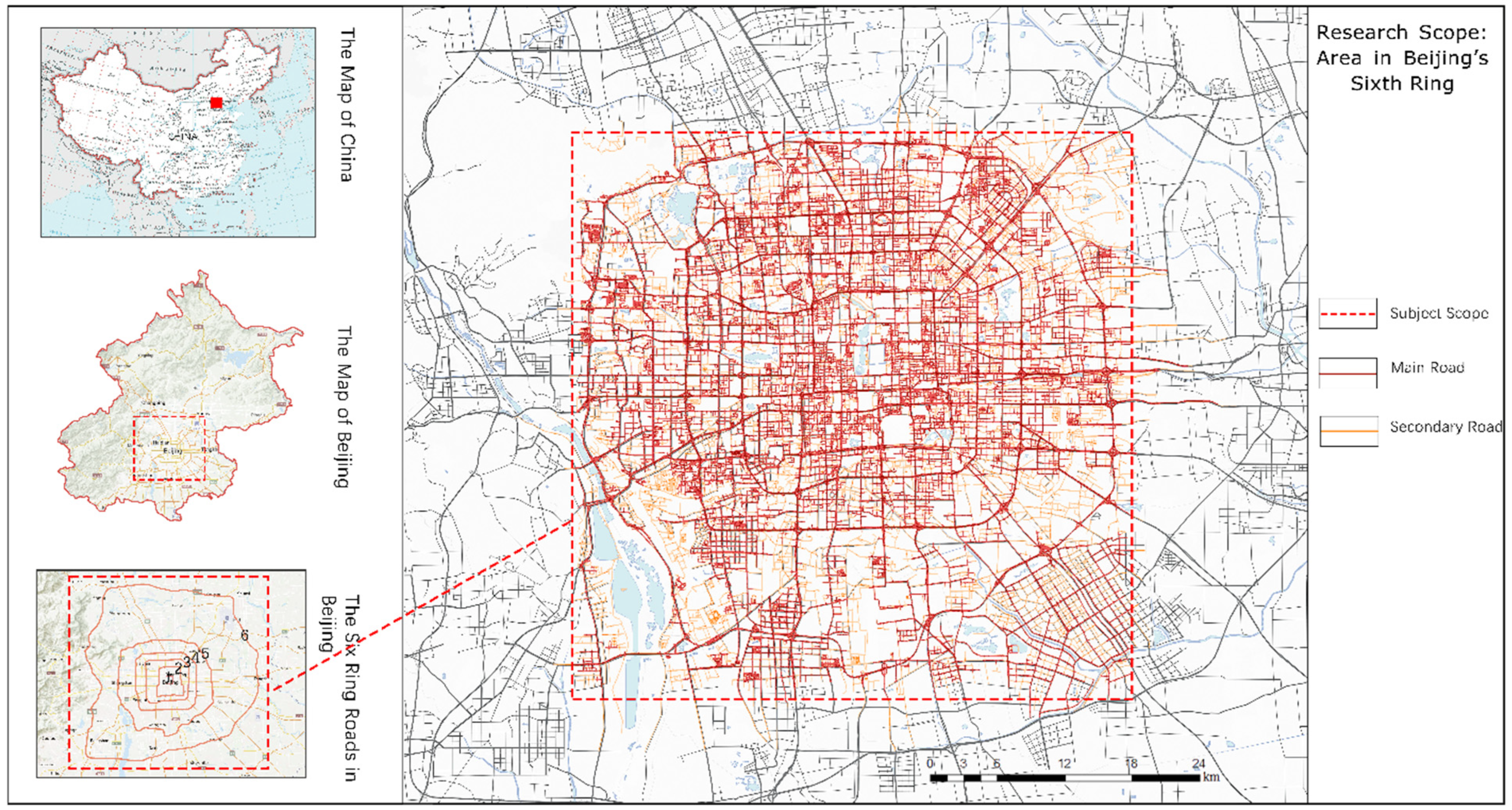
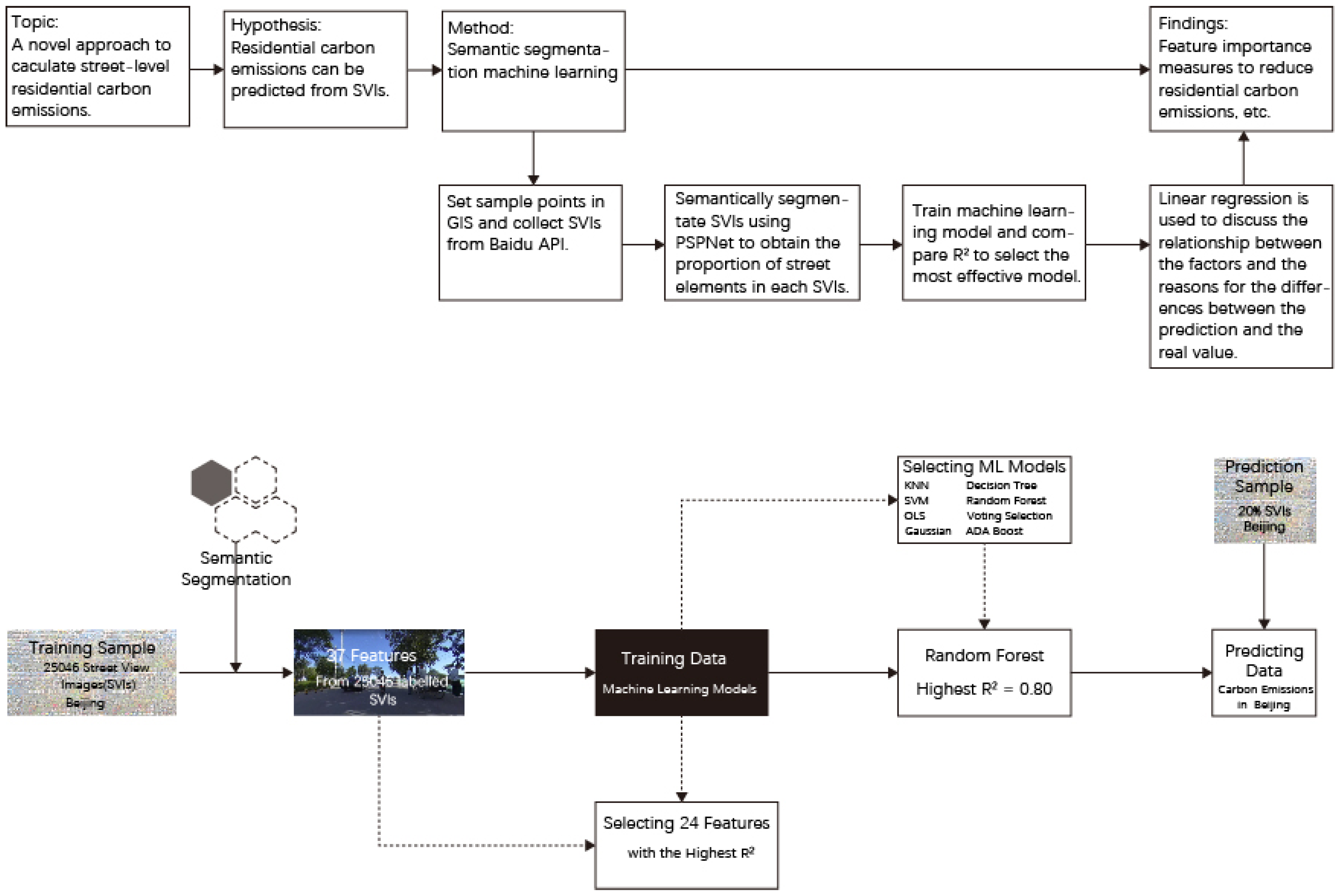
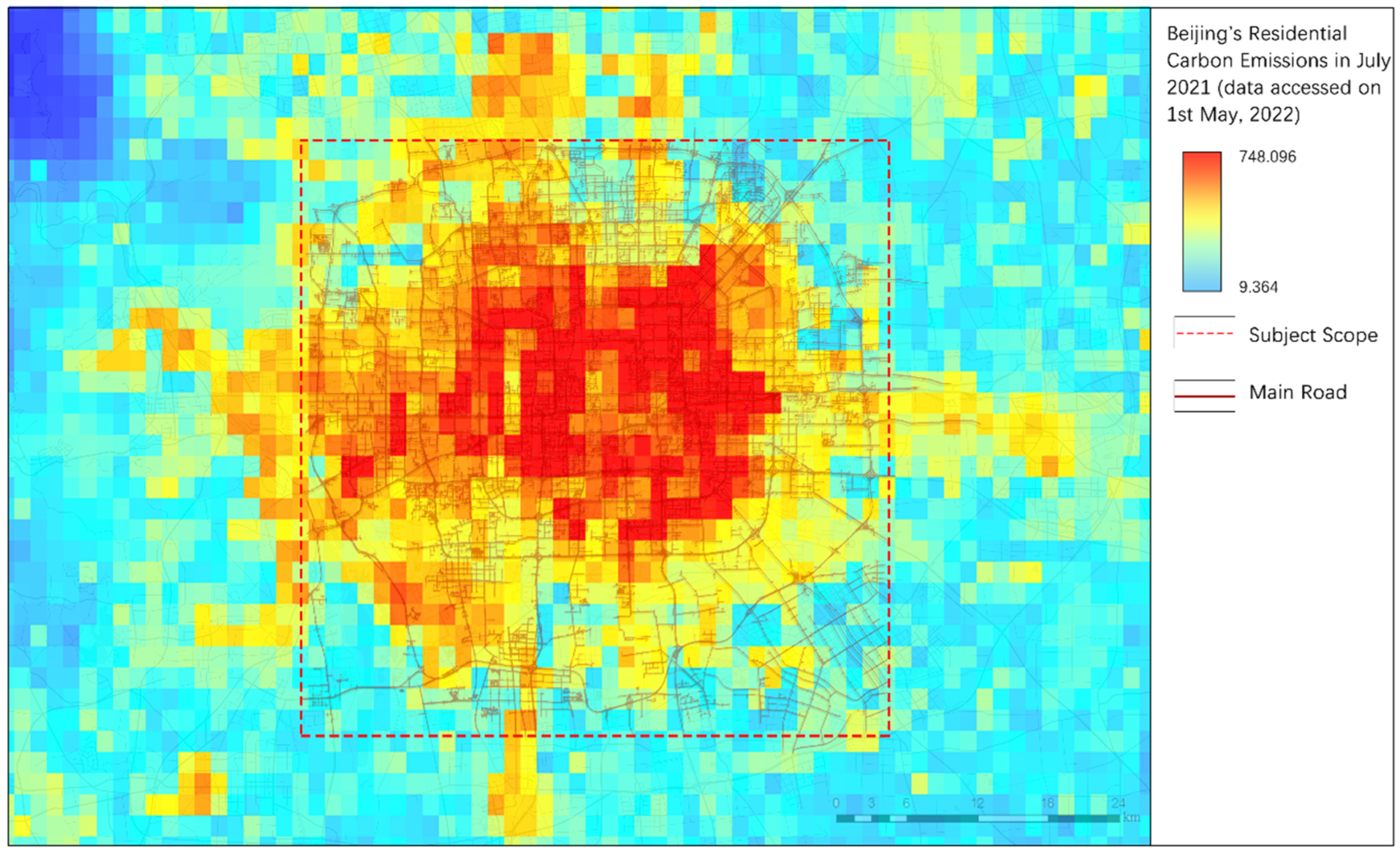
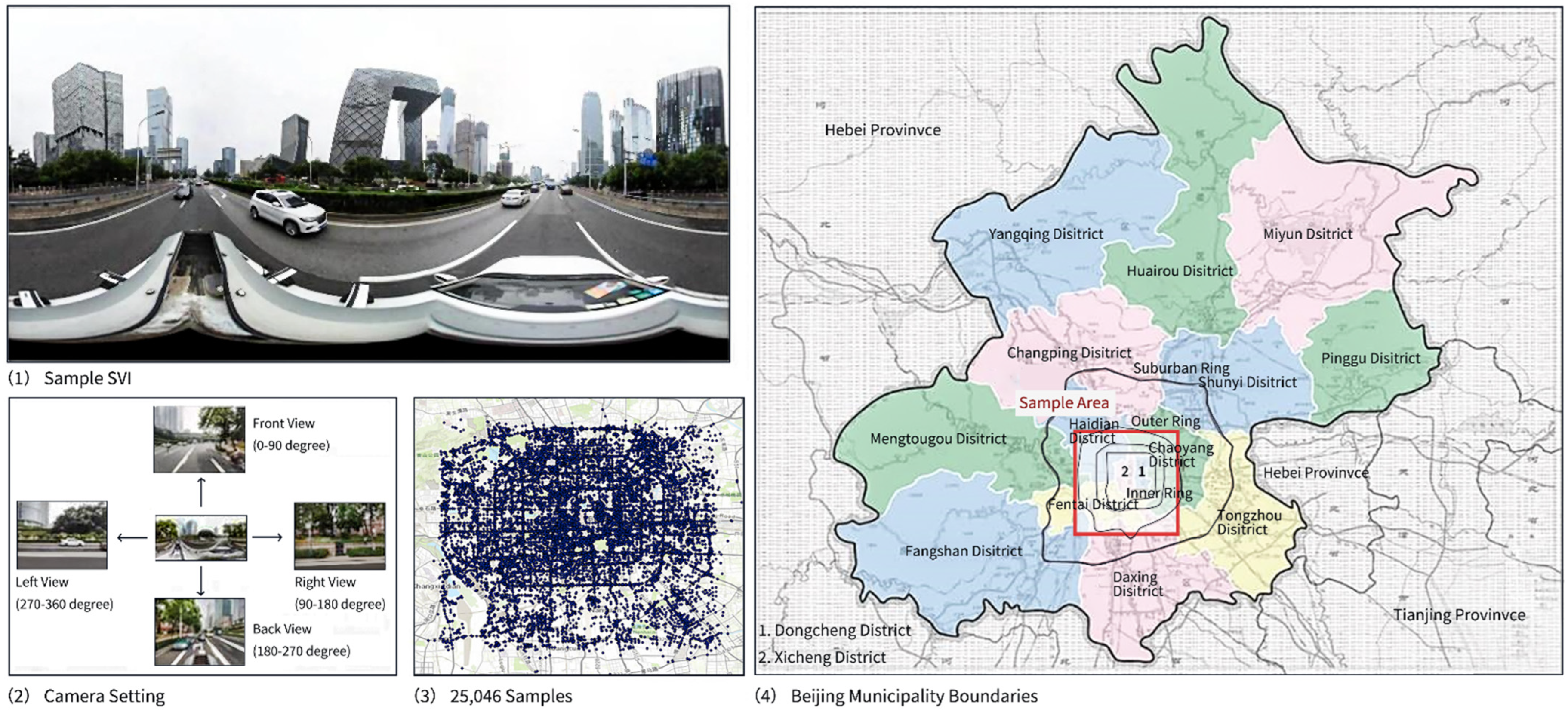
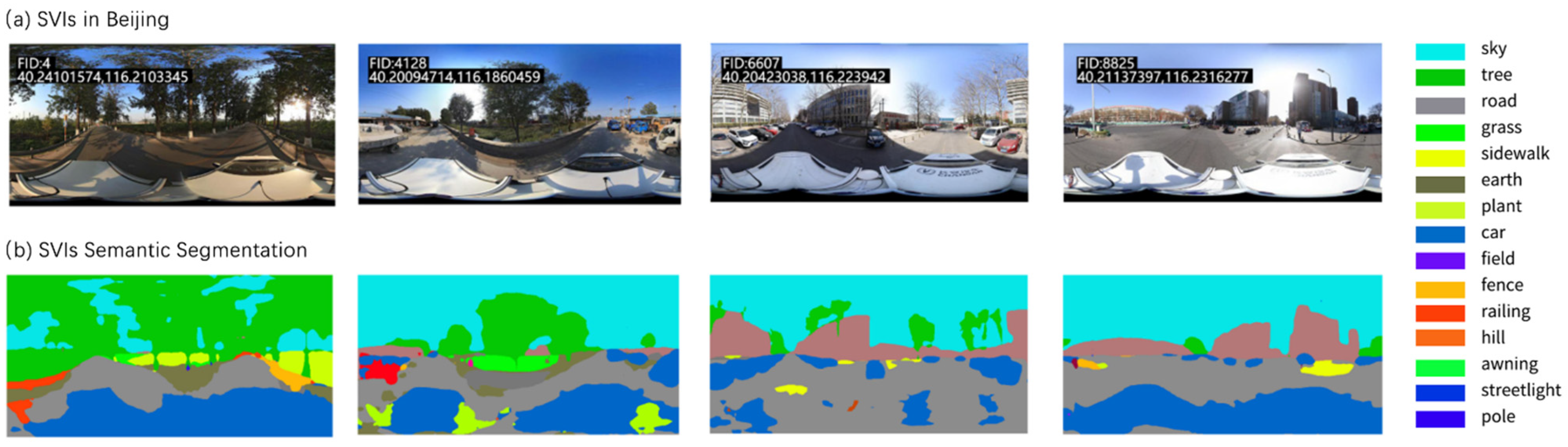
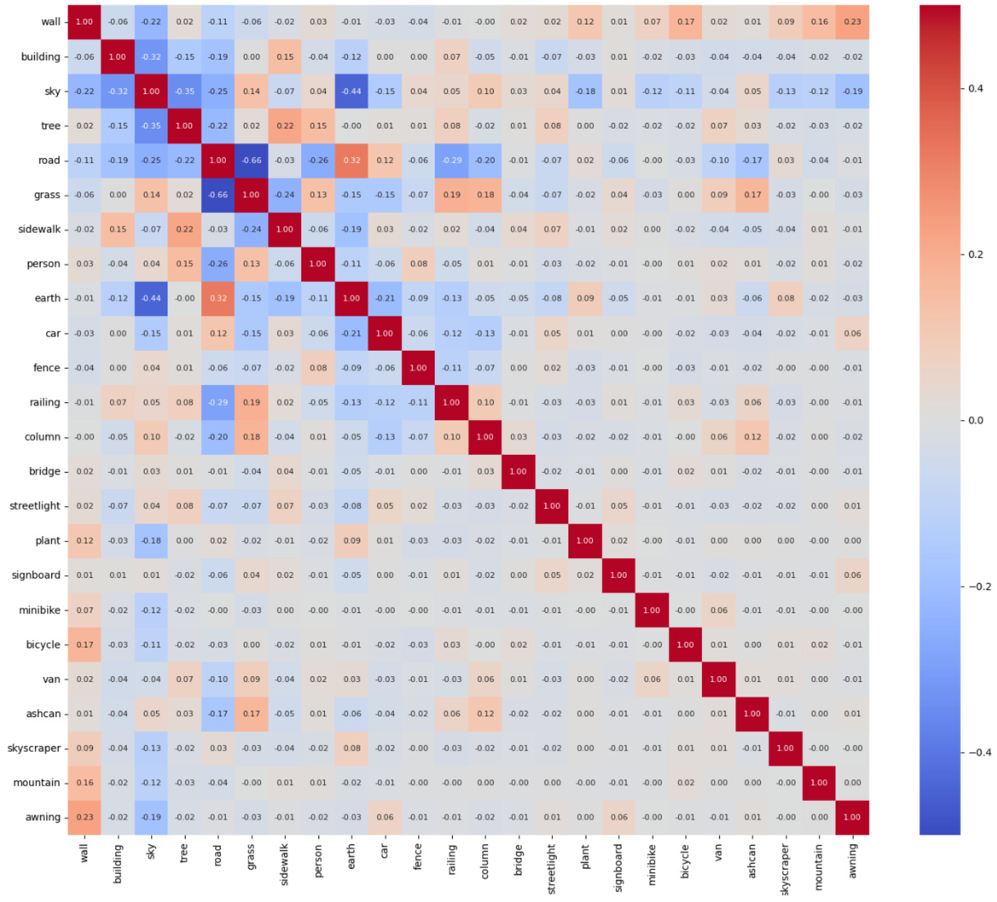
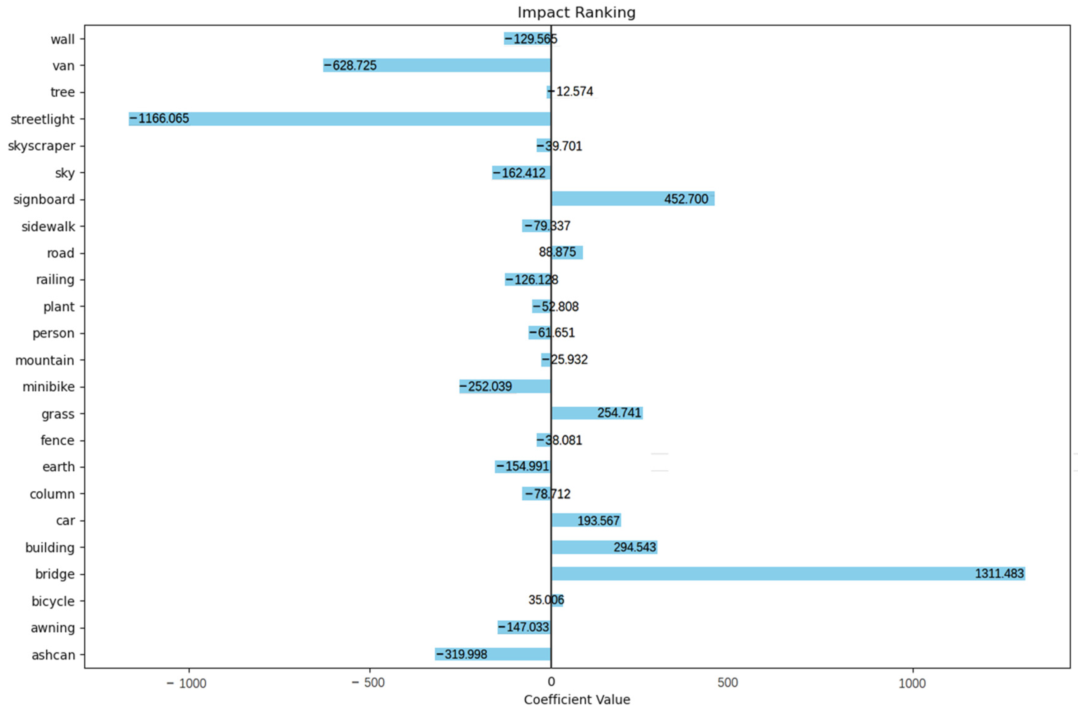
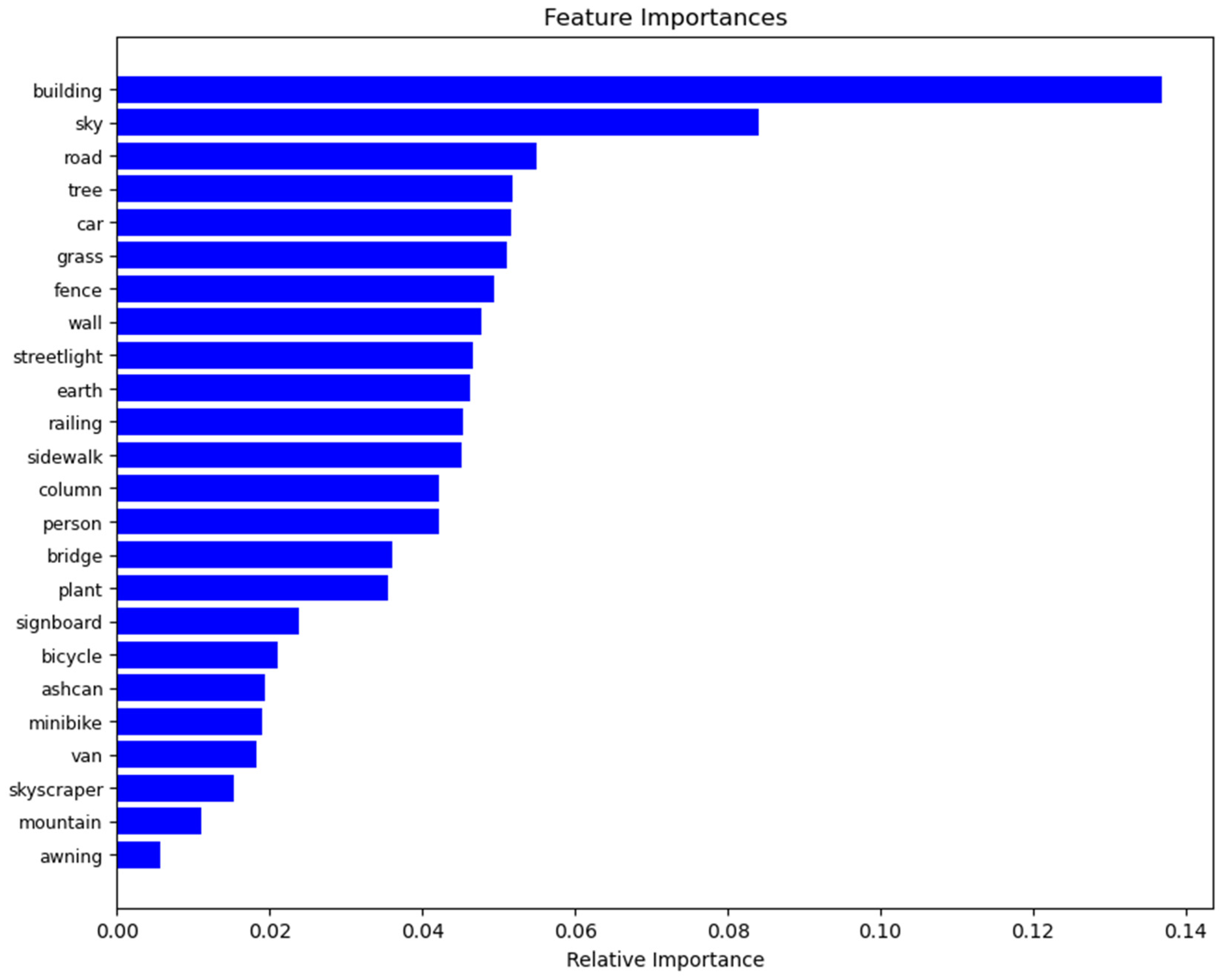
Predicting Neighborhood-Level Residential Carbon Emissions from Street View Images Using Computer Vision and Machine Learning
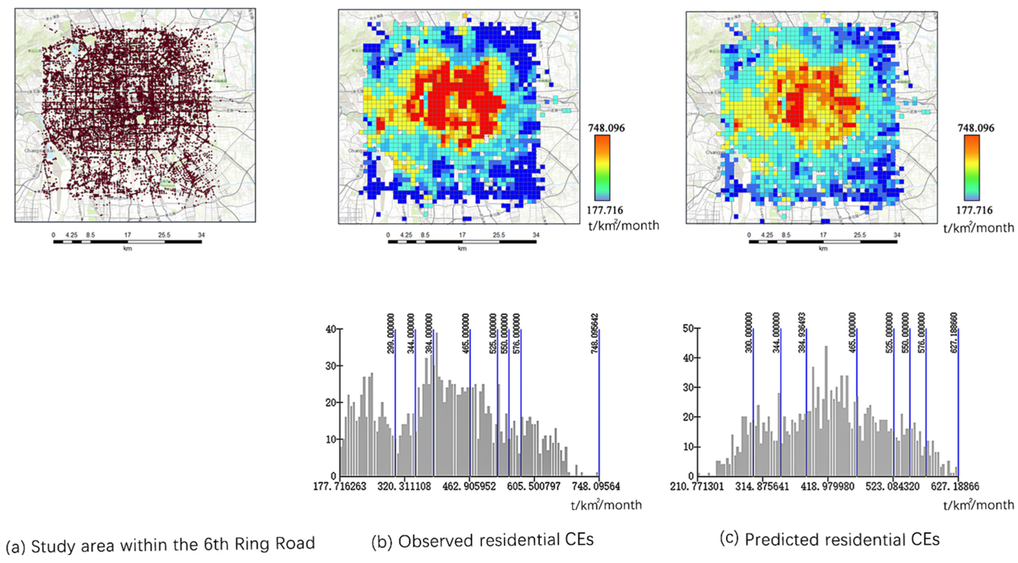
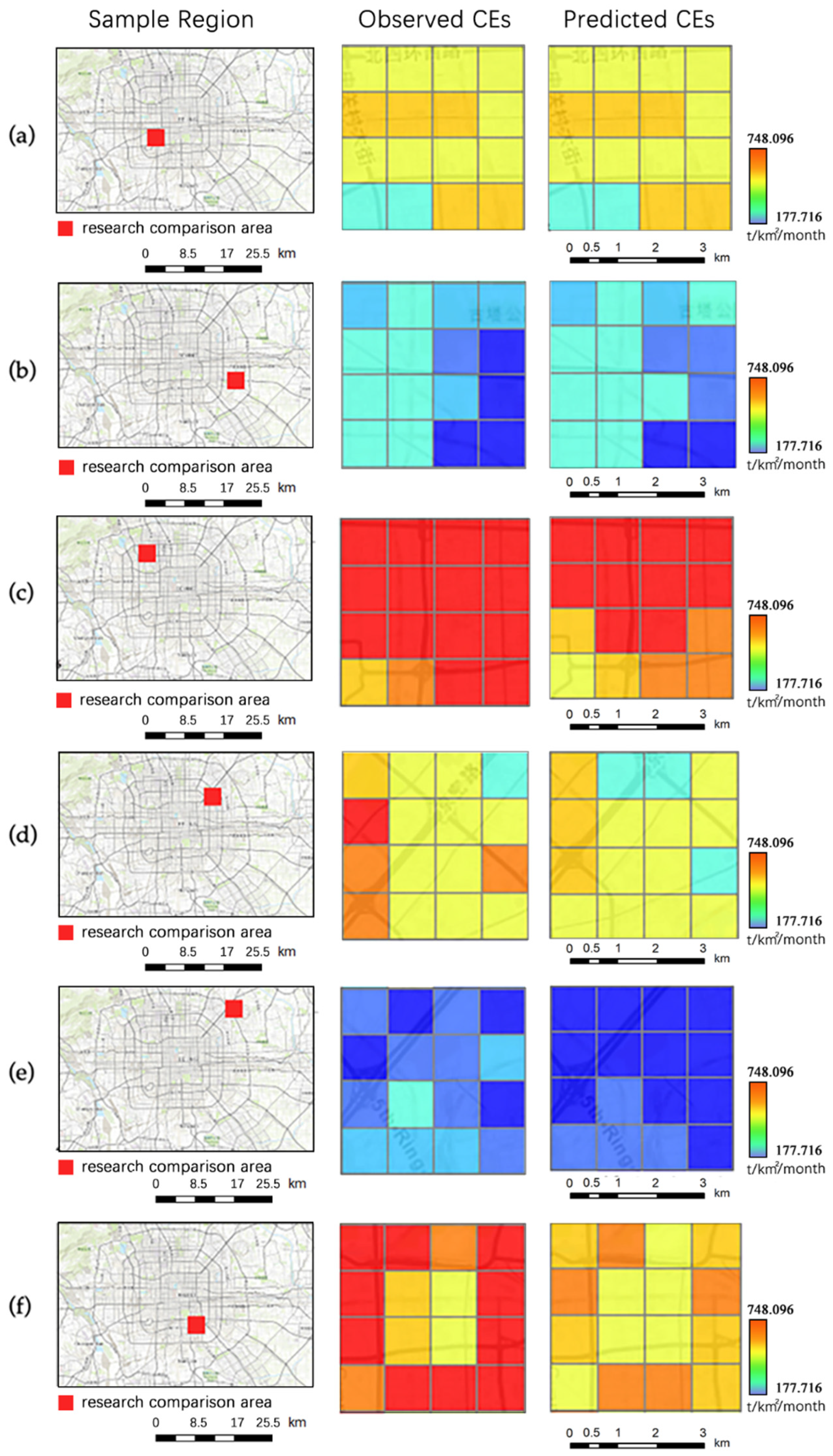
1
School of Architecture, Royal College of Art, London SW7 2EU, UK
2
The Bartlett, UCL Faculty of the Built Environment, University College London, London WC1E 6BT, UK
3
College of Civil Engineering and Architecture, Zhejiang University, Hangzhou 310058, China
4
College of Environmental Design, UC Berkeley, Berkeley, CA 94720, USA
5
Department of Urban Planning and Design, The University of Hong Kong, Hong Kong, China
*
Author to whom correspondence should be addressed.
These authors contributed equally to this work.
Remote Sens. 2024, 16(8), 1312; https://doi.org/10.3390/rs16081312
Submission received: 31 January 2024 / Revised: 1 April 2024 / Accepted: 2 April 2024 / Published: 9 April 2024
(This article belongs to the Special Issue Urban Sensing Methods and Technologies II)

Abstract

:
Predicting urban-scale carbon emissions (CEs) is crucial in drawing implications for various urgent environmental issues, including global warming. However, prior studies have overlooked the impact of the micro-level street environment, which might lead to biased prediction. To fill this gap, we developed an effective machine learning (ML) framework to predict neighborhood-level residential CEs based on a single data source, street view images (SVIs), which are publicly available worldwide. Specifically, more than 30 streetscape elements were classified from SVIs using semantic segmentation to describe the micro-level street environment, whose visual features can indicate major socioeconomic activities that significantly affect residential CEs. A ten-fold cross-validation was deployed to train ML models to predict the residential CEs at the 1 km grid level. We found, first, that random forest (R2 = 0.8) outperforms many traditional models, confirming that visual features are non-negligible in explaining CEs. Second, more building, wall, and fence views indicate higher CEs. Third, the presence of trees and grass is inversely related to CEs. Our findings justify the feasibility of using SVIs as a single data source to effectively predict neighborhood-level residential CEs. The framework is applicable to large regions across diverse urban forms, informing urban planners of sustainable urban form strategies to achieve carbon-neutral goals, especially for the development of new towns.

1. Introduction

1.1. Urban Form and CEs

Carbon emissions (CEs) from fossil fuels (e.g., paraffin, gas, coal, and other natural gas) have driven global climate change [1,2], resulting in more frequent natural disasters [3] and causing potable water [4] and energy insecurities [5]. Being one of the main emitters [6], China generates about 10 billion tons of CEs annually, accounting for roughly one-third of total global emissions [7]. In reaction, China commits to achieve the “3060” goal, with CE reduction measures across many sectors [8,9]. Notably, the residential sector is the second-largest emitter, which accounts for 23% of the Total Final Consumption (TFC) of fossil fuels [10,11]. Moreover, as the urban population grew rapidly from 170 million to 670 million between 1978 and 2010, China’s urbanization rate remarkably soared from 18% to 50% [12]. The lifecycle energy consumption of the high urban population will play a crucial role in drawing implications for predicting residential CEs [13,14,15].
Consequently, for China to successfully transform to a low-carbon economy, neighborhood-level CE reduction measures become essential [16]. The neighborhood is a basic spatial unit that accommodates urban dwellers and their daily socioeconomic activities—a microcosm of the urbanization process [17]. Therefore, the neighborhood-level urban form inherently implies the region’s efficiency regarding the allocation and utilization of energy resources [18]. That said, we hypothesize that the neighborhood-level urban form directly and indirectly influences CEs through its multi-dimensional indicators, such as the land use and building density. Understand the interlinkages would inform a more sustainable urban development to achieve the CE reduction goal [19].
Understanding how the urban form affects CEs requires the capability to accurately model greenhouse gas concentrations. It also requires a comprehensive dataset to capture factors influencing CEs at the individual and regional levels [20]. However, it has long been challenging to model the complex urban environment, which is highly variable in space and time [21,22]. Specifically, this study aims to tackle the following three gaps.

1.2. Knowledge Gap

To start with, the data sources for CE models are limited. Traditionally, predicting residential CEs relies on multifaceted GIS data—energy consumption as well as socioeconomic and demographic datasets (e.g., the census and a household economics survey)—to build regression models. However, detailed energy consumption data are not available in many cities; they do not even exist for small cities due to insufficient funding for CE data collection, nor do fine-grained sociodemographic data exist everywhere [23]. Energy consumption data are often at the city scale rather than at the mesoscale [24]. Additionally, socioeconomic data often come from different periods than energy consumption data. Therefore, conventional CE prediction models are not immediately applicable to a new region or a different period [25].
Moreover, modeling accuracy is often limited given the increased complexity of urban form variables. Scholars use complex data sources in the hopes of capturing the dynamic socioeconomic situations related to CEs, yet this could be counterproductive [26,27]. Oftentimes, multiple sources are deployed to generate multifaceted independent variables (e.g., land use, residential density, travel mode choice, and traffic). However, the built environment and the consequent residential activities are perpetually evolving, making it difficult to keep multi-source datasets up to date [18,28,29,30,31,32,33]. That said, building a time-effective model at the urban scale is desirable. Street view images (SVIs) are frequently updated, making them ideal open-source data [34,35,36] to describe timely changes (at least) on a yearly or even quarterly basis and therefore making them an ideal single source for CE modeling.
Additionally, the traditional model is generally built based on satellite images and GIS data, ignoring the street-level information that is more capable of modeling neighborhood-level activities. For example, satellite images are not fully capable of describing the urban form at a fine granularity, as there are many sight obstructions, e.g., tree canopies or view angles. Taking transportation CEs [37] as an example, driving trajectory data are often the source of insight in estimating traffic flows and their corresponding CEs. However, satellite images lack the traffic information for many residential blocks due to obstructions from tree canopies. However, SVIs are capable of inferring traffic information of neighborhoods; therefore, they are a promising tool in improving the accuracy of CE modeling.

1.3. Hypothesis and Research Design

Prior studies have confirmed that the built environment consists of various factors influencing residential CEs [38]. The factors range from urban greening [35,38,39], density [40], and building height and building quality [41] to public infrastructures (e.g., roads and bus stops) [42]. Notably, these factors can be inferred from SVIs. Specifically, the green view index is a proxy of greenery [43], which is important for carbon sequestration [44,45,46], while the building view index is a proxy for building density and building height [47,48], which significantly affect CEs [49]. Adequate public infrastructure and convenient transportation (e.g., roads, streetlights, and bus stops) may suggest a more walkable and bikeable neighborhood whose residents would have a higher tendency for active travel [35,50], resulting in lower CEs [42]. A more developed economy with adequate infrastructure also relates to better maintained buildings whose dwellers exhibit stronger awareness and obligation of low-carbon measures. For example, streetscapes such as walls and fences can imply the quality of the building; a more complex composition of the façade suggests a higher-quality building whose likelihood of HVAC installation is higher and whose residents’ income is higher, tending to consume more energy. In other words, streetscape features extracted from SVIs can imply abundant dweller behavior information, which can outweigh the impacts of the geometry itself to model energy use [51].
The micro-scale built environment described by SVIs is also related to other indicators of residential behaviors, including walkability [52,53], bikeability [54,55,56], running [35], public transit ridership [57], and, therefore, mode choice [58,59] and active living [60,61,62]. Moreover, SVIs can infer the urban forms like street canyons and density [63,64] that explain local climate zones [65,66,67], an effective indicator for modeling neighborhood microclimate, outdoor comfort, and urban heat island effects [68,69,70], which ultimately influence energy usage and CEs.
In terms of the feasibility of the SVI data source, Google provides publicly available API access to obtain the frequently updated SVIs, while Baidu and Tencent are dominant suppliers in China. SVIs have become a common method to replace time-consuming and costly field auditing [71,72,73,74], being easily implementable at the urban scale [75,76]. However, despite the large potential of SVIs, little has been empirically tested to justify their effectiveness. To fill in the gap, this paper proposes an image-based framework to directly predict residential CEs based on the micro-level streetscape features extracted from the SVI dataset.

2. Literature Review

2.1. Conventional Urban Energy Models

Conventional urban CE models can be classified into three families based on methodology: (1) models that directly measure the CO2 concentration from remote-sensed satellite data, for example, the TanSat Satellite [77]; (2) models that aggregate sectoral emission data collected from sensors monitoring viable spatial grids ranging from a city to a household, among which “one square kilometer” is the most common resolution [78]; (3) models that relate the global CE data to human societal indicators in smaller spatial units [79].
The first approach mainly translates observed spectral data into the distribution of carbon dioxide, thereby obtaining global- or regional-scale carbon flux information. It becomes a key source for observing global and regional CO2 distributions [80,81]. Publicly accessible satellite datasets include Europe’s SCIAMACHY, the USA’s OCO-2 and OCO-3, Japan’s GOSAT and GOSAT-2, and China’s TanSat [77]. Recent studies have showcased the capability to map and estimate regional CO2 emissions [82] as well as facility-scale CH4 fluxes in urban and complex areas [83,84]. This method exclusively yields CO2 emission data based on advancements in satellite technology, and its disadvantages are as evident as its merits: it offers frequent updates for the global coverage in atmospheric CO2 levels.
The second approach collects carbon data from sensors [85,86] or simulated energy consumption and CEs [87] including the fuel consumption conversion based on prior sensor data [88]. It often determines the total CEs of a given region based on fossil energy consumption information disaggregated by sectors—this is particularly prevalent in China. For example, China’s National Greenhouse Gas Inventory is created by experts from various fields within the National Development and Reform Commission. They developed the “Provincial Greenhouse Gas Inventory Compilation Guidelines (PGGICG)” in 2011, comprising sectors including waste disposal, land-use changes, forestry, agriculture, production processes, and industrial and energy activities. A recent study in the US [89] quantified CEs from fossil fuel consumptions by sectors with a bottom–up method and measured hourly emissions from citywide industrial/electricity facilities, road segments, and individual buildings. Notably, various datasets, such as building energy simulations, electricity production data, traffic insights, and local pollution reports, were merged to build the dataset. City sub-regions can also be modeled. For example, ref. [90] measured the energy-use intensity (EUI) for each building type using the building energy efficiency monitoring platform in Shanghai. Ref. [91] incorporated a traffic allocation model to mimic traffic situations using a gasoline consumption function—the User Equilibrium (UE). Although their method versatility suits major cities in the more developed world, it is not immediately applicable to medium-to-small-sized cities in many developing countries where no similar data source exists.
The third approach disaggregates global CE data to a finer resolution relating to the indicators describing the built environment and industrial activities. This is because there was a strong alignment between the surface fluxes of atmospheric CO2 and bottom–up inventories [92,93] or urban activity indicators like land use [94,95] and road length [96]. On the one hand, nighttime light (NTL) images are found to reflect human activities correlated with energy consumption. Therefore, the brightness of NTL pixels significantly correlates with CEs, enabling the prediction across spatial and temporal scales. On the other hand, various urban layers, such as transportation networks [97,98], buildings [99,100,101], and households [102,103], are related to the CE prediction [104]. Other explanatory factors include population [105] and living standards [14]. This approach is particularly useful for the ex-ante assessment of alternative urban scenarios to support decisions like urban retrofitting aiming at achieving low-carbon goals [17,106].

2.2. SVIs for Urban Form Modeling

Multifaceted natural, socioeconomic, and human behavior forces have made neighborhood-level residential CE prediction challenging [107]. Fortunately, with the rapid improvements in AI and multi-source big data applications for urban studies, many urban form characteristics that are used to model CEs have become more accessible to researchers [108]. Some focus on the complex relationships between total urban CEs and the industrial/economic development level or urban sprawl trend of the region [109,110]. Some other studies consider the regularity of historical data [111]—the cyclical trends in CE. For example, ref. [112] studied the influence of household members’ environmental perceptions and energy consumption behavior on household CEs. More recently, ref. [113] modeled household travel patterns from neighborhoods’ urban forms to evaluate CEs. An increasing number of models have started to address the interplay between people’s energy-use habits and the environment they live in.
Meanwhile, SVI data are publicly available and frequently updated to capture ground-level panorama street scenes [114]. SVIs are an ideal dataset to comprehensively describe the urban environmental variability [115] and citizen behaviors, including building height [116], streetscape features [117], green and water systems [118], land-use classification [94,119,120], openness [121], road networks [122], mobile monitoring [98], mobility patterns [123,124], sun-glare-related traffic crashes [125], land use [79,126,127,128], and residential behavior [129].
Among these urban environment characteristics and societal consequences, many are related directly or indirectly to energy consumption, indicating significant correlations with CE estimation. To the best of our knowledge, few studies have attempted to parse SVIs to module urban-scale CEs. Only one recent study took SVIs to model household-travel CEs in Jinan, China [130]. However, in this study, SVIs only represent the road and road–building relationship (i.e., urban canyon). To fill in the research gap, this study sets out to address the effectiveness of using SVI data to capture urban forms related to the energy-use behaviors of citizens as latent layers to predict residential CEs.

3. Data and Method

3.1. Analytical Framework

3.1.1. Study Area

Beijing, as the capital city and one of the largest metropolitan areas in China, is crucial in addressing the CE reduction goal. Moreover, its diverse urban forms ranging from the central business district (CBD), residential blocks, and industry parks to the periphery, with its massive road network, provide important samples in addressing the effectiveness of our proposed framework. Within the Sixth Ring Road is the area where most urban residents live. This region has the most frequent urban mobility and resident activities. Therefore, the area within the Sixth Ring Road in Beijing was chosen (Figure 1).

3.1.2. Conceptual Framework

The framework consists of six steps (see Figure 2). First, remote-sensing CE data were provided by Planet Data Tech (Suzhou) Ltd., a car-bon data platform company based on satellite quantitative remote sensing fusion algorithm and high-quality environmental data model, with a 1 km level data grid. Second, the SVIs were obtained, using Baidu Open Platform API (https://lbsyun.baidu.com/, accessed on 1 May 2022) in Python 3.8 through the coordinates of the selected points along the road network in Beijing at a 250 m interval. For each sampling coordinate, we obtained the 360-degree-view SVI. Third, PSPNet, a semantic segmentation model, was used to extract the proportion of various street elements from each SVI. The most ubiquitous visual elements related to CEs suggested by the literature, including the surface, sidewalk, greenery, sky, road, building, wall, fence, and seat, were selected. Fourth, training of ML models was performed to predict CEs using visual features extracted in Python. The goodness of fit (R2) was chosen as the criterion to select the most accurate models from the four ML models (i.e., KNN, SVM, random forest, and decision trees). Last, we used the trained ML model to predict the residential CEs in Beijing, visualizing the gaps between the ground-truth CE and our best prediction to validate our model and understand the potential causes of the biases based on the impact ranking and feature importance.

3.2. Variables

3.2.1. Residential Carbon Emissions

The residential CEs in July 2021 (the most available year at the time this study was initiated) were provided by Planet Data Tech (Suzhou) Ltd., and with the tagged image file (TIF) of residential CEs in a 1 km grid (data accessed on 22 April 2022). The CE estimation comes from Tsinghua University’s MEIC CE data inventory. By relating urban activity indicators (e.g., energy consumption and the number of residents per area) with the original satellite CE data (at the 1/4° resolution), Planet Data established a 1 km resolution CE model (1/100°) covering all the urban regions in China using a fusion model.
Ideally, it is preferrable to have the CE and SVI data collected during the same period of the year such that the seasonal variations of the street environments will be captured. However, since the focus of this paper is to demonstrate the usefulness of predicting CEs from a single data source (i.e., SVIs), we decided to predict a random month’s CE values as an initial test. Notably, since SVIs are mostly collected in spring and summer (March to August), to align the CE data as much as possible with the SVIs regarding collecting time, July’s data are appropriate for an initial case study (Figure 3).

3.2.2. Independent Variables

SVI Data Collection

Baidu Street View images represent the most significant data source available for use in studying urban streets. Several different angles of street view images are available using Baidu Maps, which is one of the largest online map providers in China. Since Google Maps is unavailable in China, Baidu Maps is an excellent choice with relatively high quality. This study downloaded Baidu Street View (BSV) imagery using the BSV API (http://api.map.baidu.com/panorama/v2, accessed on 1 May 2022)). We set the sampling point to capture street view images in four radial directions at a fixed height, giving a total of 25,046 street view images (Figure 4) based on our sampling points every 250 m along the road networks. Each image had a resolution of 512 × 512 pixels and was in JPG format, making them a reliable source for our research. Note that (by checking the time data) all SVI samples were taken during 2019–2021, being the most up-to-date dataset that is available to match the period of our CE data. We looked through the street view history in Baidu Maps, which makes it possible for users to see how a place has changed over the years and help identify changes in the physical environment. There were few major construction projects in the study area during this period. Considering that the street environment is rather stable in the short term [131], we were able to assume no significant changes happened during the sample period (2019–2021). Notably, the SVI retrieval process is also consistent with all parameters, including the heading, the position coordinates (longitude and latitude), the image resolution (width and height), the horizontal field, and the pitch.

Semantic Segmentation

The independent variables are streetscape visual features extracted from the 25,046 SVIs (Figure 4). Streetscape features represent the micro-level built environment that becomes hidden layers to represent comprehensive urban information related to residential CEs, such as urban location, land use, microclimate condition, and residents’ behavior such as their living styles and habits, which link to the residential CEs.
PSPNet (Pyramid Scene Parsing Network), a deep learning (DL) semantic segmentation tool, was used to process the SVIs. Semantic segmentation refers to dividing and parsing images into several areas linked with semantic categories [132]. PSPNet has become a commonly used approach in emerging urban studies to extract street canyon characteristics [133,134,135] and has shown state-of-the-art performance on the ADE20K database, achieving an accuracy of over 80% [133,136].
Consequently, for each SVI, the output is the visual feature’s view index, denoting the pixel percentage of the feature identified to the total pixels of the image. More than 30 visual features were observed from all SVI samples in Beijing (Figure 5), including natural features (e.g., tree and grass), built environment features (e.g., road, sidewalk, and building), and traffic features (e.g., car, bus, bicycle). Evidently, not all visual elements should be taken as independent variables. Variables whose presences in SVIs were minor were removed.
To this end, the residential CEs at each SVI sample point become the dependent variable, while the selected visual features’ view indices become the independent variables for all the 25,046 SVIs (Table 1) to train the ML models for prediction.

3.3. Model Architecture

3.3.1. Machine Learning Models

Since the number of independent variables is less than 40, ML models might be more suitable than the neural network model. Regarding the ML training, 80% of the sample was used for training and 20% for validation. The training utilizes a ten-fold cross-validation approach deployed to add effectiveness to the models’ training. Specifically, the input data were divided into 10 subgroups: for each iteration, one subgroup was utilized as the testing data while the other nine subgroups were employed for training. In other words, all data were utilized to train the ML models after 10 iterations, therefore lowering the bias. What is more, every iteration’s model weights for the convolutional layers are continuously updated, which also adds to the effectiveness of training [137].

3.3.2. Training Algorithm

Before training, we employed a method to identify and remove outliers from the SAMPLE residential column, the Interquartile Range (IQR), a common statistical approach for outlier detection to enhance the quality of our dataset and to ensure robust analysis. Instead of the traditional 25th (Q1) and 75th (Q3) percentiles, we opted for the 30th and 70th percentiles to compute the IQR. After the outlier removal process, approximately 99.57% of the original data remained. This process ensured that our analyses were conducted on a dataset free from extreme values that might skew the results.
In our research, we applied eight commonly used ML models to train and predict carbon data based on the SVIs. To identify the optimal ML model, we conducted experiments to evaluate their performances against established metrics, which are regarded as indicative of the most efficient ML models [138]. During the training process, the accuracy of ML models was evaluated using the R2 (correlation coefficient), RMSE (root mean square error), MAE (mean absolute error), and IA (index of agreement). Whereas the R2 represents the goodness of fit, the IA is representative of the agreement of the estimated value with the observed value, and the fitting effect of the MAE and RMSE is representative of the deviation of the estimated value from the observed value.
Simultaneously, the choice of visual elements was also determined while applying interactions. All visual elements were first used as test objects for all ML models, which resulted in the highest R2 among all ML models as the baseline model. Then, the feature importance of each element was considered as the criterion for screening. The elements with the lowest feature importance in the model performance were removed in turn, and then the model performance after removal was compared with the model performance before removal, and finally the element combination with the best performance was obtained.

4. Results and Discussions

4.1. Analysis of Results

4.1.1. Model Performance

After training, we obtained the best performance of the model with 24 elements as the input. Table 2 shows the comparison of the performance of the eight ML models. Among them, the model using the random forest algorithm had the best performance, which leverages the collective outputs of multiple decision trees to generate a unified result. Its inherent simplicity and flexibility have facilitated its widespread adoption, particularly in handling large datasets and yielding precise predictions for both classification and regression tasks. It had the best performance and obtained an R2 of 0.80021, while the model’s RMSE was 58.11 t/km2/month, and its MAE was 40.90 t/km2/month.

4.1.2. Co-linearity Issues

The pairwise correlation analysis illustrates potential co-linearity issues among the streetscape visual features (Figure 6). Highly correlated variables will be further investigated with reference to the VIF test (Table 3) and literature on CE estimation to decide whether they should be t removed. For example, “earth” and “road” are highly related, raising concerns for the multicollinearity issue. However, the test suggests a VIF < 10, while both “earth” and “road” are important indicators for different aspects affecting the residential energy use. The “road” indicates travel models and mobility/accessibility related to travel frequency and travel mode, while the “earth” affects land surface permeability and the micro-climate. Therefore, both streetscapes were kept.

4.1.3. The Roles of Micro-Level Built Environment Visual Features

The impact factor (IF) and feature importance (FI) analysis revealed a big divergence regarding what visual features are significant in predicting the CEs. On the one hand, the IF ranking (based on linear regression coefficients) indicates that bridge, streetlight, van, signboard, ashcan, building, grass, minibike, car, sky, and earth were the most impactful (Figure 7). On the other hand, the FI analysis highlights divergent visual elements as more effective when using tree-based ML models (Figure 8). The top 10 features regarding FI are building, sky, road, tree, car, grass, fence, wall, streetlight, and earth. Given that the OLS has a significantly poorer performance (Table 2), the relationship between visual features and the CEs is more likely to be non-linear. The FI analysis is more reliable.
The FI analysis shows that features such as building, sky, road, tree, car, grass, fence, and wall are in strong correlation with CEs (Figure 8). This is reasonable, as a higher ratio of these elements can indicate a higher residential density, resulting in more frequent socioeconomic activities that consume energy. For instance, the high ratio of building view can indicate the frequent use of air conditioners. Such a phenomenon may be even more significant in our study since the CE data used were collected in July. The average temperature in Beijing was 29 °C when household cooling appliances were widely used. Moreover, a higher density of residents will also lead to an increased use of vehicles. As another example, more road views in SVIs could suggest higher traffic volumes, resulting in greater CEs in the urban region.
In addition, a greater view index of buildings, walls, and fences suggests narrower urban canyons, which reduce wind speeds and can slow down the diffusion of carbon-containing gases, keeping the CE value sensed at a relatively higher level than that in open streets. Meanwhile, Choi et al. (2016) found that block-scaled UFP (ultrafine particle) concentrations have a close connection with the surface turbulence and built environment of buildings in urban areas [139]. And CEs are also in the form of particles in the air and are related to construction in the streets.

4.2. Discussion

4.2.1. Spatial and Temporal Distribution of Residential CEs

In general, high values of CEs happen in densely populated areas, such as the center of the city. The CEs of residents in diverse microenvironments shows significant spatial heterogeneity. For example, the unit CEs of suburban areas around Beijing are the lowest, with the CEs in July ranging from 106 to 211 t/km2/month, while the unit CEs are higher closer to the center of the city where the density of residents is high. The total CEs in July were between 177.72 and 748.10 t/km2/month. In the eastern urban districts of Beijing, such as Chaoyang and Dongcheng, the overall CEs in residential areas in summer are higher than those in the western urban districts, such as Changping and Haidian. This is probably because the eastern urban area is an old urban area, with more resident activities and a higher population density, resulting in more CEs.
Therefore, the CEs in Beijing residential areas present obvious spatial heterogeneity in their distribution. Meanwhile, the density of residents and their activity frequencies can be directly reflected from the street view. This is because residents’ activities largely shape the SVIs. For example, in general, a place with a higher population density has more resident activities, more residential buildings, and a higher building density, which then demonstrates as less greenery and more bounding walls. In addition, a place with more resident activities and a higher population has more vehicles in the SVIs. Therefore, the street map can be used to predict residents’ CEs and reflect the spatial heterogeneity of residents’ CE accordingly.

4.2.2. Model Visualization and Model Application Scenarios

To better visualize the CE prediction results, ArcGIS was used to illustrate the difference between actual and predicted residential CE values within each 1 km grid (Figure 9). The actual CE value ranged between 177 and 748 t/km2/month; therefore, the estimated CEs were also visualized at the same scale, to be more immediately comparable.
Figure 10 clearly depicts a relatively reliable prediction of CE values, as overall there are no distinct divergences between the predicted and actual CE values. However, certain deviations were observed across the Beijing urban area. Notably, a significant portion of the city registered lower predicted CEs than the actual recorded values. Interestingly, this trend shifts at the urban fringes, where our model consistently predicts higher emissions than what has been observed. This variance could be indicative of underlying complexities in the urban peripheral dynamics that may not be fully encapsulated by the current model. These findings are invaluable, highlighting potential areas of refinement in our predictive mechanisms, especially concerning the nuanced interplay at the city’s outskirts. Figure 9 indicates that prediction accuracy is higher when the ground truth value falls in a certain range (350–550 t/km2/month). When the actual CEs are low and high, the accuracy of the predicted values will be low. The range of actual CEs is 177.72–748.10 t/km2/month, while the predicted range is 210.77–627.19 t/km2/month.
Given the spatial heterogeneity of prediction residual, we selected six areas of 16-square-kilometer urban areas to investigate the divergence between the actual and predicted data. These six areas are distributed in various parts of Beijing (Figure 10). Among them, the MAEs in Figure 10a,b,d are smaller, indicating better prediction accuracy. It can be seen from the comparison of Figure 10c,e that there exist quite great gaps in the prediction of the extremely high value and extremely low value, and the accuracy does not perform well. Figure 10f is similar to the average level, but there is still a certain gap when predicting higher CE values.

4.2.3. Model Comparison

To the best of our knowledge, currently, there are only a few mesoscale residential CE models [140]. As a cross-reference validation, we selected three similar studies that also focus on household residential and travel CEs to compare with our CE model (Table 4). In comparison to the existing literature, our study stands out for its innovative approach and remarkable accuracy in predicting residential carbon emissions. While previous studies have utilized a plethora of data sources, ranging from socioeconomic indicators to land-use patterns and geographic variables, our model achieves comparable performance using variables derived from SVIs. This highlights the efficiency and potential of leveraging simpler data sources for carbon emissions predictions.
That said, this study not only proposed a model that can better predict residents’ carbon emissions on a small scale, but more importantly, we verified the possibility of using street view, a simple data source, to predict residents’ carbon emissions, supporting simpler data sources for a wide geographical region. A more timely and finer-grained carbon emissions prediction model can be potentially established for cities where data availability is limited, especially those in developing countries.

5. Conclusions and Limitations

5.1. Effects of Micro-Level Streetscape Attributes

This study developed an innovative framework to predict residential CEs in urban areas, leveraging SVIs and ML techniques. Our study underscores the feasibility of incorporating micro-level urban streetscape elements into CE prediction models to address the gaps in existing carbon emissions prediction models.
We first explained the relationship between residential CEs and built environment characteristics, and how streetscape elements represent urban regional characteristics through literature reviews, thereby drawing a possible correlation between streetscape elements and urban residential carbon emissions. By employing a semantic segmentation algorithm, we classified 32 outdoor streetscape elements from SVIs and obtained the best-performing random forest prediction model composed of 24 street view elements, such as buildings, trees, and sky through multiple iterative comparisons, whose R2 is 0.8. Notably, our findings indicate that the ratios of elements including bridge, signboard, road, grass, car, building, and bicycle, which indicate dense urban features, are correlated with higher emissions. Conversely, streetlight, van, etc., demonstrate a negative relationship with CEs. In addition, building, sky, and road have the highest feature importance among all features.
This study contributes to the field by demonstrating the relative importance of various streetscape elements in CE prediction and showcasing the model’s potential for generalization across different urban contexts. It also offers a novel perspective for CE prediction using a single, open data source but also provides a valuable tool for urban planners and policymakers. Our findings suggest that understanding the interplay between urban design and CEs can inform sustainable and low-carbon urban development strategies. The streetscape elements can be conducive to the creation of urban environments under the concept of low-carbon design, and the visual nature of our model empowers citizens to engage in public decision making and urban living choices. This will let the goals of sustainable development and carbon neutrality gain a foothold to be promoted and optimized on a large scale.

5.2. Limitations

However, our research has limitations. First, we only modeled one month’s data, meaning that we failed to control for whether the vegetation is green or not, which might result in different SVI analyses and a different model fit to explain CEs. It would be ideal to collect solid information on the periods when SVIs were collected so as to model seasonal variations in the street environment. That said, future studies can accumulate time-series data and build separate models by season. In the meantime, microclimates can also be taken into consideration. Microclimates have regional characteristics. People may adopt more energy-efficient appliances or pursue a more comfortable temperature environment in different buildings. Therefore, microclimates have a certain impact on residential energy consumption and carbon emissions [143,144]. In the future, we can try to use the microclimate as one of the impact factors for the optimization of the prediction model. Third, as carbon emissions distributions were found to be heterogeneous, there were differences according to urban functional zone (UFZ) types [25]. Comparing the different SVI features and the differences in CEs of the specific areas in Chaoyang, including the prosperous areas with high population densities, CBD areas, suburbs, industrial areas, etc., is beneficial in discussing the model’s transferability in different urban scenarios and could possibly increase the mobility and accuracy of the model in different regions. The aforementioned limitations could be addressed to examine more spatial effects on residential CEs in the future.

Author Contributions

W.S. and Y.X. contributed equally to this manuscript. Conceptualization, Y.X. and W.S.; methodology, W.S. and R.Z.; software, Y.J. and W.S.; validation, Y.J.; formal analysis, W.S.; investigation, Y.Y.; resources, Y.Y.; data curation, Y.J.; writing—original draft preparation, W.S., Y.X., and Y.J.; writing—review and editing, W.S. and Y.X.; visualization, W.S. and Y.X.; supervision, W.Q.; project administration, W.Q. All authors have read and agreed to the published version of the manuscript.

Funding

This research received no external funding.

Data Availability Statement

The data presented in this study are available on request from the corresponding author.

Acknowledgments

Thanks Wenjing Li (The University of Tokyo), Xun Liu (University of Virginia), and Da Chen (University of Bath) for their helps with the preliminary analysis.

Conflicts of Interest

The authors declare no conflicts of interest.

References

  1. Du, K.; Li, J. Towards a Green World: How Do Green Technology Innovations Affect Total-Factor Carbon Productivity. Energy Policy 2019, 131, 240–250. [Google Scholar] [CrossRef]
  2. Qian, L.; Xu, X.; Sun, Y.; Zhou, Y. Carbon Emission Reduction Effects of Eco-Industrial Park Policy in China. Energy 2022, 261, 125315. [Google Scholar] [CrossRef]
  3. Shi, C.; Guo, N.; Gao, X.; Wu, F. How Carbon Emission Reduction Is Going to Affect Urban Resilience. J. Clean. Prod. 2022, 372, 133737. [Google Scholar] [CrossRef]
  4. Huang, C.; Tao, J. Chapter 4—Water-Related Problems with Special Reference to Global Climate Change in China. In Water Conservation and Wastewater Treatment in BRICS Nations; Singh, P., Milshina, Y., Tian, K., Gusain, D., Bassin, J.P., Eds.; Elsevier: Amsterdam, The Netherlands, 2020; pp. 61–82. ISBN 978-0-12-818339-7. [Google Scholar]
  5. Ryu, H.; Dorjragchaa, S.; Kim, Y.; Kim, K. Electricity-Generation Mix Considering Energy Security and Carbon Emission Mitigation: Case of Korea and Mongolia. Energy 2014, 64, 1071–1079. [Google Scholar] [CrossRef]
  6. Liu, J.; Li, S.; Ji, Q. Regional Differences and Driving Factors Analysis of Carbon Emission Intensity from Transport Sector in China. Energy 2021, 224, 120178. [Google Scholar] [CrossRef]
  7. Joint Research Centre (European Commission); Crippa, M.; Guizzardi, D.; Schaaf, E.; Monforti-Ferrario, F.; Quadrelli, R.; Risquez Martin, A.; Rossi, S.; Vignati, E.; Muntean, M.; et al. GHG Emissions of All World Countries: 2023; Publications Office of the European Union: Luxembourg, 2023; ISBN 978-92-68-07550-0. [Google Scholar]
  8. CSC. The Fourteenth Five-Year Plan; China’s State Council: Beijing, China, 2021.
  9. He, W.; Liu, D.; Wang, C. Are Chinese Provincial Carbon Emissions Allowances Misallocated over 2000–2017? Evidence from an Extended Gini-Coefficient Approach. Sustain. Prod. Consum. 2022, 29, 564–573. [Google Scholar] [CrossRef]
  10. Fan, J.-L.; Liao, H.; Liang, Q.-M.; Tatano, H.; Liu, C.-F.; Wei, Y.-M. Residential Carbon Emission Evolutions in Urban–Rural Divided China: An End-Use and Behavior Analysis. Appl. Energy 2013, 101, 323–332. [Google Scholar] [CrossRef]
  11. Yuan, X.; Wang, X.; Zuo, J. Renewable Energy in Buildings in China—A Review. Renew. Sustain. Energy Rev. 2013, 24, 1–8. [Google Scholar] [CrossRef]
  12. Chen, M.; Liu, W.; Tao, X. Evolution and Assessment on China’s Urbanization 1960–2010: Under-Urbanization or over-Urbanization? Habitat Int. 2013, 38, 25–33. [Google Scholar] [CrossRef]
  13. Park, H.-C.; Heo, E. The Direct and Indirect Household Energy Requirements in the Republic of Korea from 1980 to 2000—An Input–Output Analysis. Energy Policy 2007, 35, 2839–2851. [Google Scholar] [CrossRef]
  14. Baiocchi, G.; Minx, J.; Hubacek, K. The Impact of Social Factors and Consumer Behavior on Carbon Dioxide Emissions in the United Kingdom. J. Ind. Ecol. 2010, 14, 50–72. [Google Scholar] [CrossRef]
  15. Cao, M.; Kang, W.; Cao, Q.; Sajid, M.J. Estimating Chinese Rural and Urban Residents’ Carbon Consumption and Its Drivers: Considering Capital Formation as a Productive Input. Environ. Dev. Sustain. 2020, 22, 5443–5464. [Google Scholar] [CrossRef]
  16. Cheng, J.; Mao, C.; Huang, Z.; Hong, J.; Liu, G. Implementation Strategies for Sustainable Renewal at the Neighborhood Level with the Goal of Reducing Carbon Emission. Sustain. Cities Soc. 2022, 85, 104047. [Google Scholar] [CrossRef]
  17. Zhang, T.; Song, Y.; Yang, J. Relationships between Urbanization and CO2 Emissions in China: An Empirical Analysis of Population Migration. PLoS ONE 2021, 16, e0256335. [Google Scholar] [CrossRef] [PubMed]
  18. Wang, S.; Wang, J.; Fang, C.; Li, S. Estimating the Impacts of Urban Form on CO2 Emission Efficiency in the Pearl River Delta, China. Cities 2019, 85, 117–129. [Google Scholar] [CrossRef]
  19. Zheng, Y.; Cheng, L.; Wang, Y.; Wang, J. Exploring the Impact of Explicit and Implicit Urban Form on Carbon Emissions: Evidence from Beijing, China. Ecol. Indic. 2023, 154, 110558. [Google Scholar] [CrossRef]
  20. Kumar, A.; Kumar, A.; Chaturvedi, A.K.; Joshi, N.; Mondal, R.; Malyan, S.K. Greenhouse Gas Emissions from Hydroelectric Reservoirs: Mechanistic Understanding of Influencing Factors and Future Prospect. Environ. Sci. Pollut. Res. 2023. [CrossRef]
  21. Jordan, M.I.; Mitchell, T.M. Machine Learning: Trends, Perspectives, and Prospects. Science 2015, 349, 255–260. [Google Scholar] [CrossRef]
  22. Helm, J.M.; Swiergosz, A.M.; Haeberle, H.S.; Karnuta, J.M.; Schaffer, J.L.; Krebs, V.E.; Spitzer, A.I.; Ramkumar, P.N. Machine Learning and Artificial Intelligence: Definitions, Applications, and Future Directions. Curr. Rev. Musculoskelet. Med. 2020, 13, 69–76. [Google Scholar] [CrossRef]
  23. Cai, M.; Shi, Y.; Ren, C.; Yoshida, T.; Yamagata, Y.; Ding, C.; Zhou, N. The Need for Urban Form Data in Spatial Modeling of Urban Carbon Emissions in China: A Critical Review. J. Clean. Prod. 2021, 319, 128792. [Google Scholar] [CrossRef]
  24. Du, R.; Liu, C.-H.; Li, X.-X. A New Method for Detecting Urban Morphology Effects on Urban-Scale Air Temperature and Building Energy Consumption under Mesoscale Meteorological Conditions. Urban Clim. 2024, 53, 101775. [Google Scholar] [CrossRef]
  25. Zheng, Y.; Du, S.; Zhang, X.; Bai, L.; Wang, H. Estimating Carbon Emissions in Urban Functional Zones Using Multi-Source Data: A Case Study in Beijing. Build. Environ. 2022, 212, 108804. [Google Scholar] [CrossRef]
  26. Bolón-Canedo, V.; Remeseiro, B. Feature Selection in Image Analysis: A Survey. Artif. Intell. Rev. 2020, 53, 2905–2931. [Google Scholar] [CrossRef]
  27. Kabir, H.; Garg, N. Machine Learning Enabled Orthogonal Camera Goniometry for Accurate and Robust Contact Angle Measurements. Sci. Rep. 2023, 13, 1497. [Google Scholar] [CrossRef] [PubMed]
  28. Ou, J.; Liu, X.; Li, X.; Chen, Y. Quantifying the Relationship between Urban Forms and Carbon Emissions Using Panel Data Analysis. Landsc. Ecol. 2013, 28, 1889–1907. [Google Scholar] [CrossRef]
  29. Ou, J.; Liu, X.; Wang, S.; Xie, R.; Li, X. Investigating the Differentiated Impacts of Socioeconomic Factors and Urban Forms on CO2 Emissions: Empirical Evidence from Chinese Cities of Different Developmental Levels. J. Clean. Prod. 2019, 226, 601–614. [Google Scholar] [CrossRef]
  30. Fang, C.; Wang, S.; Li, G. Changing Urban Forms and Carbon Dioxide Emissions in China: A Case Study of 30 Provincial Capital Cities. Appl. Energy 2015, 158, 519–531. [Google Scholar] [CrossRef]
  31. Shu, X.; Xia, C.; Li, Y.; Tong, J.; Shi, Z. Relationships between carbon emission, urban growth, and urban forms of urban agglomeration in the Yangtze River Delta. Ecol. Indic. 2018, 38, 6302–6313. [Google Scholar] [CrossRef]
  32. Shi, K.; Xu, T.; Li, Y.; Chen, Z.; Gong, W.; Wu, J.; Yu, B. Effects of Urban Forms on CO2 Emissions in China from a Multi-Perspective Analysis. J. Environ. Manag. 2020, 262, 110300. [Google Scholar] [CrossRef]
  33. Qiu, W.; Li, W.; Liu, X.; Zhang, Z.; Li, X.; Huang, X. Subjective and Objective Measures of Streetscape Perceptions: Relationships with Property Value in Shanghai. Cities 2023, 132, 104037. [Google Scholar] [CrossRef]
  34. Qiu, W.; Zhang, Z.; Liu, X.; Li, W.; Li, X.; Xu, X.; Huang, X. Subjective or Objective Measures of Street Environment, Which Are More Effective in Explaining Housing Prices? Landsc. Urban Plan. 2022, 221, 104358. [Google Scholar] [CrossRef]
  35. Dong, L.; Jiang, H.; Li, W.; Qiu, B.; Wang, H.; Qiu, W. Assessing Impacts of Objective Features and Subjective Perceptions of Street Environment on Running Amount: A Case Study of Boston. Landsc. Urban Plan. 2023, 235, 104756. [Google Scholar] [CrossRef]
  36. Su, N.; Li, W.; Qiu, W. Measuring the Associations between Eye-Level Urban Design Quality and on-Street Crime Density around New York Subway Entrances. Habitat Int. 2023, 131, 102728. [Google Scholar] [CrossRef]
  37. Xia, C.; Xiang, M.; Fang, K.; Li, Y.; Ye, Y.; Shi, Z.; Liu, J. Spatial-Temporal Distribution of Carbon Emissions by Daily Travel and Its Response to Urban Form: A Case Study of Hangzhou, China. J. Clean. Prod. 2020, 257, 120797. [Google Scholar] [CrossRef]
  38. Shen, Y.-S.; Lin, Y.-C.; Cui, S.; Li, Y.; Zhai, X. Crucial Factors of the Built Environment for Mitigating Carbon Emissions. Sci. Total Environ. 2022, 806, 150864. [Google Scholar] [CrossRef] [PubMed]
  39. Vaccari, F.P.; Gioli, B.; Toscano, P.; Perrone, C. Carbon Dioxide Balance Assessment of the City of Florence (Italy), and Implications for Urban Planning. Landsc. Urban Plan. 2013, 120, 138–146. [Google Scholar] [CrossRef]
  40. Liu, X.; Ou, J.; Chen, Y.; Wang, S.; Li, X.; Jiao, L.; Liu, Y. Scenario Simulation of Urban Energy-Related CO2 Emissions by Coupling the Socioeconomic Factors and Spatial Structures. Appl. Energy 2019, 238, 1163–1178. [Google Scholar] [CrossRef]
  41. Tranchard, S. Measuring the Carbon Footprint of Buildings in a Simple Way. Available online: https://www.iso.org/cms/render/live/en/sites/isoorg/contents/news/2017/07/Ref2205.html (accessed on 26 January 2024).
  42. Zhang, J.; Zhang, L.; Qin, Y.; Wang, X.; Zheng, Z. Influence of the Built Environment on Urban Residential Low-Carbon Cognition in Zhengzhou, China. J. Clean. Prod. 2020, 271, 122429. [Google Scholar] [CrossRef]
  43. Lu, Y.; Ferranti, E.J.S.; Chapman, L.; Pfrang, C. Assessing Urban Greenery by Harvesting Street View Data: A Review. Urban For. Urban Green. 2023, 83, 127917. [Google Scholar] [CrossRef]
  44. Dwyer, J.F.; Nowak, D.J.; Noble, M.H.; Sisinni, S.M. Connecting People with Ecosystems in the 21st Century: An Assessment of Our Nation’s Urban Forests.; U.S. Department of Agriculture, Forest Service, Pacific Northwest Research Station: Portland, OR, USA, 2000; p. PNW-GTR-490.
  45. Nowak, D.J.; Crane, D.E. Carbon Storage and Sequestration by Urban Trees in the USA. Environ. Pollut. 2002, 116, 381–389. [Google Scholar] [CrossRef]
  46. Birge, D.; Mandhan, S.; Qiu, W.; Berger, A.M. Potential for Sustainable Use of Trees in Hot Arid Regions: A Case Study of Emirati Neighborhoods in Abu Dhabi. Landsc. Urban Plan. 2019, 190, 103577. [Google Scholar] [CrossRef]
  47. Carrasco-Hernandez, R.; Smedley, A.R.D.; Webb, A.R. Using Urban Canyon Geometries Obtained from Google Street View for Atmospheric Studies: Potential Applications in the Calculation of Street Level Total Shortwave Irradiances. Energy Build. 2015, 86, 340–348. [Google Scholar] [CrossRef]
  48. Gong, F.-Y.; Zeng, Z.-C.; Zhang, F.; Li, X.; Ng, E.; Norford, L.K. Mapping Sky, Tree, and Building View Factors of Street Canyons in a High-Density Urban Environment. Build. Environ. 2018, 134, 155–167. [Google Scholar] [CrossRef]
  49. Resch, E.; Bohne, R.A.; Kvamsdal, T.; Lohne, J. Impact of Urban Density and Building Height on Energy Use in Cities. Energy Procedia 2016, 96, 800–814. [Google Scholar] [CrossRef]
  50. Li, W.; Joh, K. Exploring the Synergistic Economic Benefit of Enhancing Neighbourhood Bikeability and Public Transit Accessibility Based on Real Estate Sale Transactions. Urban Stud. 2017, 54, 3480–3499. [Google Scholar] [CrossRef]
  51. Quan, S.J.; Wu, J.; Wang, Y.; Shi, Z.; Yang, T.; Yang, P.P.-J. Urban Form and Building Energy Performance in Shanghai Neighborhoods. Energy Procedia 2016, 88, 126–132. [Google Scholar] [CrossRef]
  52. Wu, F.; Li, W.; Qiu, W. Examining Non-Linear Relationship between Streetscape Features and Propensity of Walking to School in Hong Kong Using Machine Learning Techniques. J. Transp. Geogr. 2023, 113, 103698. [Google Scholar] [CrossRef]
  53. Ha, J.; Ki, D.; Lee, S.; Ko, J. Mode Choice and the First-/Last-Mile Burden: The Moderating Effect of Street-Level Walkability. Transp. Res. Part Transp. Environ. 2023, 116, 103646. [Google Scholar] [CrossRef]
  54. Ito, K.; Biljecki, F. Assessing Bikeability with Street View Imagery and Computer Vision. Transp. Res. Part C Emerg. Technol. 2021, 132, 103371. [Google Scholar] [CrossRef]
  55. Qiu, W.; Chang, H. The Interplay between Dockless Bikeshare and Bus for Small-Size Cities in the US: A Case Study of Ithaca. J. Transp. Geogr. 2021, 96, 103175. [Google Scholar] [CrossRef]
  56. Song, Q.; Li, W.; Li, J.; Wei, X.; Qiu, W. Disclosing the Impact of Micro-Level Environmental Characteristics on Dockless Bikeshare Trip Volume: A Case Study of Ithaca. In Proceedings of the Intelligence for Future Cities; Goodspeed, R., Sengupta, R., Kyttä, M., Pettit, C., Eds.; Springer Nature Switzerland: Cham, Switzerland, 2023; pp. 125–147. [Google Scholar]
  57. Su, S.; Wang, Z.; Li, B.; Kang, M. Deciphering the Influence of TOD on Metro Ridership: An Integrated Approach of Extended Node-Place Model and Interpretable Machine Learning with Planning Implications. J. Transp. Geogr. 2022, 104, 103455. [Google Scholar] [CrossRef]
  58. Koo, B.W.; Guhathakurta, S.; Botchwey, N.; Hipp, A. Can Good Microscale Pedestrian Streetscapes Enhance the Benefits of Macroscale Accessible Urban Form? An Automated Audit Approach Using Google Street View Images. Landsc. Urban Plan. 2023, 237, 104816. [Google Scholar] [CrossRef]
  59. Wu, W.; Yao, Y.; Wang, R. Green Space Exposure at Subway Stations, Transportation Mode Choice and Travel Satisfaction. Transp. Res. Part Transp. Environ. 2023, 122, 103862. [Google Scholar] [CrossRef]
  60. Sallis, J.F.; Cervero, R.B.; Ascher, W.; Henderson, K.A.; Kraft, M.K.; Kerr, J. An Ecological Approach to Creating Active Living Communities. Annu. Rev. Public Health 2006, 27, 297–322. [Google Scholar] [CrossRef]
  61. Steinmetz-Wood, M.; Velauthapillai, K.; O’Brien, G.; Ross, N.A. Assessing the Micro-Scale Environment Using Google Street View: The Virtual Systematic Tool for Evaluating Pedestrian Streetscapes (Virtual-STEPS). BMC Public Health 2019, 19, 1246. [Google Scholar] [CrossRef] [PubMed]
  62. Tan, Y.; Li, W.; Chen, D.; Qiu, W. Identifying Urban Park Events through Computer Vision-Assisted Categorization of Publicly-Available Imagery. ISPRS Int. J. Geo-Inf. 2023, 12, 419. [Google Scholar] [CrossRef]
  63. Middel, A.; Lukasczyk, J.; Zakrzewski, S.; Arnold, M.; Maciejewski, R. Urban Form and Composition of Street Canyons: A Human-Centric Big Data and Deep Learning Approach. Landsc. Urban Plan. 2019, 183, 122–132. [Google Scholar] [CrossRef]
  64. Qiu, W.; Li, W.; Liu, X.; Huang, X. Subjectively Measured Streetscape Perceptions to Inform Urban Design Strategies for Shanghai. ISPRS Int. J. Geo-Inf. 2021, 10, 493. [Google Scholar] [CrossRef]
  65. Cao, S.; Zhang, L.; He, Y.; Zhang, Y.; Chen, Y.; Yao, S.; Yang, W.; Sun, Q. Effects and Contributions of Meteorological Drought on Agricultural Drought under Different Climatic Zones and Vegetation Types in Northwest China. Sci. Total Environ. 2022, 821, 153270. [Google Scholar] [CrossRef] [PubMed]
  66. Ignatius, M.; Xu, R.; Hou, Y.; Liang, X.; Zhao, T.; Chen, S.; Wong, N.H.; Biljecki, F. Local Climate Zones: Lessons from Singapore and Potential Improvement with Street View Imagery. ISPRS Ann. Photogramm. Remote Sens. Spat. Inf. Sci. 2022, X-4-W2-2022, 121–128. [Google Scholar] [CrossRef]
  67. Xu, X.; Qiu, W.; Li, W.; Huang, D.; Li, X.; Yang, S. Comparing Satellite Image and GIS Data Classified Local Climate Zones to Assess Urban Heat Island: A Case Study of Guangzhou. Front. Environ. Sci. 2022, 10, 1029445. [Google Scholar] [CrossRef]
  68. Stewart, I.; Oke, T. Classifying Urban Climate Field Sites by “Local Climate Zones”: The Case of Nagano, Japan. In Proceedings of the The seventh International Conference on Urban Climate, Yokohama, Japan, 29 June–3 July 2009. [Google Scholar]
  69. Stewart, I.D.; Oke, T.R. Local Climate Zones for Urban Temperature Studies. Bull. Am. Meteorol. Soc. 2012, 93, 1879–1900. [Google Scholar] [CrossRef]
  70. Xu, C.; Chen, G.; Huang, Q.; Su, M.; Rong, Q.; Yue, W.; Haase, D. Can Improving the Spatial Equity of Urban Green Space Mitigate the Effect of Urban Heat Islands? An Empirical Study. Sci. Total Environ. 2022, 841, 156687. [Google Scholar] [CrossRef] [PubMed]
  71. Rundle, A.G.; Bader, M.D.M.; Richards, C.A.; Neckerman, K.M.; Teitler, J.O. Using Google Street View to Audit Neighborhood Environments. Am. J. Prev. Med. 2011, 40, 94–100. [Google Scholar] [CrossRef] [PubMed]
  72. Griew, P.; Hillsdon, M.; Foster, C.; Coombes, E.; Jones, A.; Wilkinson, P. Developing and Testing a Street Audit Tool Using Google Street View to Measure Environmental Supportiveness for Physical Activity. Int. J. Behav. Nutr. Phys. Act. 2013, 10, 103. [Google Scholar] [CrossRef] [PubMed]
  73. Kelly, C.M.; Wilson, J.S.; Baker, E.A.; Miller, D.K.; Schootman, M. Using Google Street View to Audit the Built Environment: Inter-Rater Reliability Results. Ann. Behav. Med. 2013, 45, S108–S112. [Google Scholar] [CrossRef] [PubMed]
  74. Queralt, A.; Molina-García, J.; Terrón-Pérez, M.; Cerin, E.; Barnett, A.; Timperio, A.; Veitch, J.; Reis, R.; Silva, A.A.P.; Ghekiere, A.; et al. Reliability of Streetscape Audits Comparing On-street and Online Observations: MAPS-Global in 5 Countries. Int. J. Health Geogr. 2021, 20, 6. [Google Scholar] [CrossRef] [PubMed]
  75. Salesses, P.; Schechtner, K.; Hidalgo, C.A. The Collaborative Image of The City: Mapping the Inequality of Urban Perception. PLoS ONE 2013, 8, e68400. [Google Scholar] [CrossRef] [PubMed]
  76. Dubey, A.; Naik, N.; Parikh, D.; Raskar, R.; Hidalgo, C.A. Deep Learning the City: Quantifying Urban Perception at a Global Scale. In Proceedings of the Computer Vision—ECCV 2016, Amsterdam, The Netherlands, 11–14 October 2016; Leibe, B., Matas, J., Sebe, N., Welling, M., Eds.; Springer International Publishing: Cham, Switzerland, 2016; pp. 196–212. [Google Scholar]
  77. Hong, X.; Zhang, P.; Bi, Y.; Liu, C.; Sun, Y.; Wang, W.; Chen, Z.; Yin, H.; Zhang, C.; Tian, Y.; et al. Retrieval of Global Carbon Dioxide From TanSat Satellite and Comprehensive Validation With TCCON Measurements and Satellite Observations. IEEE Trans. Geosci. Remote Sens. 2022, 60, 1–16. [Google Scholar] [CrossRef]
  78. Gregg, J.S.; Andres, R.J. A Method for Estimating the Temporal and Spatial Patterns of Carbon Dioxide Emissions from National Fossil-Fuel Consumption. Tellus B Chem. Phys. Meteorol. 2008, 60, 1–10. [Google Scholar] [CrossRef]
  79. Huang, W.; Cui, L.; Chen, M.; Zhang, D.; Yao, Y. Estimating Urban Functional Distributions with Semantics Preserved POI Embedding. Int. J. Geogr. Inf. Sci. 2022, 36, 1905–1930. [Google Scholar] [CrossRef]
  80. Crisp, D. Measuring CO2 from Space: The NASA Orbiting Carbon Observatory-2. In Proceedings of the 61st International Astronautical Congress (IAC 2010), Prague, Czech Republic, 27 September–1 October 2010. [Google Scholar]
  81. Yoshida, Y.; Ota, Y.; Eguchi, N.; Kikuchi, N.; Nobuta, K.; Tran, H.; Morino, I.; Yokota, T. Retrieval Algorithm for CO2 and CH4 Column Abundances from Short-Wavelength Infrared Spectral Observations by the Greenhouse Gases Observing Satellite. Atmospheric Meas. Tech. 2011, 4, 717–734. [Google Scholar] [CrossRef]
  82. Hakkarainen, J.; Ialongo, I.; Tamminen, J. Direct Space-Based Observations of Anthropogenic CO2 Emission Areas from OCO-2. Geophys. Res. Lett. 2016, 43, 11,400–11,406. [Google Scholar] [CrossRef]
  83. Thompson, D.R.; Thorpe, A.K.; Frankenberg, C.; Green, R.O.; Duren, R.; Guanter, L.; Hollstein, A.; Middleton, E.; Ong, L.; Ungar, S. Space-Based Remote Imaging Spectroscopy of the Aliso Canyon CH4 Superemitter. Geophys. Res. Lett. 2016, 43, 6571–6578. [Google Scholar] [CrossRef]
  84. Frankenberg, C.; Berry, J. 3.10—Solar Induced Chlorophyll Fluorescence: Origins, Relation to Photosynthesis and Retrieval. In Comprehensive Remote Sensing; Liang, S., Ed.; Elsevier: Oxford, UK, 2018; pp. 143–162. ISBN 978-0-12-803221-3. [Google Scholar]
  85. Christen, A. Atmospheric Measurement Techniques to Quantify Greenhouse Gas Emissions from Cities. Urban Clim. 2014, 10, 241–260. [Google Scholar] [CrossRef]
  86. Feng, L.; Palmer, P.I.; Parker, R.J.; Deutscher, N.M.; Feist, D.G.; Kivi, R.; Morino, I.; Sussmann, R. Estimates of European Uptake of CO2 Inferred from GOSAT XCO2 Retrievals: Sensitivity to Measurement Bias inside and Outside Europe. Atmospheric Chem. Phys. 2016, 16, 1289–1302. [Google Scholar] [CrossRef]
  87. Pao, H.-T.; Tsai, C.-M. Modeling and Forecasting the CO2 Emissions, Energy Consumption, and Economic Growth in Brazil. Energy 2011, 36, 2450–2458. [Google Scholar] [CrossRef]
  88. Shao, L.; Guan, D.; Zhang, N.; Shan, Y.; Chen, G.Q. Carbon Emissions from Fossil Fuel Consumption of Beijing in 2012. Environ. Res. Lett. 2016, 11, 114028. [Google Scholar] [CrossRef]
  89. Gurney, K.R.; Liang, J.; O’Keeffe, D.; Patarasuk, R.; Hutchins, M.; Huang, J.; Rao, P.; Song, Y. Comparison of Global Downscaled Versus Bottom-Up Fossil Fuel CO2 Emissions at the Urban Scale in Four U.S. Urban Areas. J. Geophys. Res. Atmospheres 2019, 124, 2823–2840. [Google Scholar] [CrossRef]
  90. Wu, H.; Guo, Z.; Peng, C. Land Use Induced Changes of Organic Carbon Storage in Soils of China. Glob. Change Biol. 2003, 9, 305–315. [Google Scholar] [CrossRef]
  91. Zhang, R.; Pu, L.; Zhu, M. Impacts of Transportation Arteries on Land Use Patterns in Urban-Rural Fringe: A Comparative Gradient Analysis of Qixia District, Nanjing City, China. Chin. Geogr. Sci. 2013, 23, 378–388. [Google Scholar] [CrossRef]
  92. Schuh, A.E.; Lauvaux, T.; West, T.O.; Denning, A.S.; Davis, K.J.; Miles, N.; Richardson, S.; Uliasz, M.; Lokupitiya, E.; Cooley, D.; et al. Evaluating Atmospheric CO2 Inversions at Multiple Scales over a Highly Inventoried Agricultural Landscape. Glob. Change Biol. 2013, 19, 1424–1439. [Google Scholar] [CrossRef]
  93. Ogle, S.M.; Davis, K.; Lauvaux, T.; Schuh, A.; Cooley, D.; West, T.O.; Heath, L.S.; Miles, N.L.; Richardson, S.; Breidt, F.J.; et al. An Approach for Verifying Biogenic Greenhouse Gas Emissions Inventories with Atmospheric CO2 Concentration Data. Environ. Res. Lett. 2015, 10, 034012. [Google Scholar] [CrossRef]
  94. Jain, A.K.; Meiyappan, P.; Richardson, T. Carbon Emissions from Land-Use Change: Model Estimates Using Three Different Data Sets. In Land Use and the Carbon Cycle: Advances in Integrated Science, Management, and Policy; Reed, B.C., Brown, D.G., Robinson, D.T., French, N.H.F., Eds.; Cambridge University Press: Cambridge, UK, 2013; pp. 241–258. ISBN 978-1-107-64835-7. [Google Scholar]
  95. Chuai, X.; Feng, J. High Resolution Carbon Emissions Simulation and Spatial Heterogeneity Analysis Based on Big Data in Nanjing City, China. Sci. Total Environ. 2019, 686, 828–837. [Google Scholar] [CrossRef] [PubMed]
  96. Song, Y.; Wu, P.; Hampson, K.; Anumba, C. Assessing Block-Level Sustainable Transport Infrastructure Development Using a Spatial Trade-off Relation Model. Int. J. Appl. Earth Obs. Geoinformation 2021, 105, 102585. [Google Scholar] [CrossRef]
  97. Ehsani, M.; Ahmadi, A.; Fadai, D. Modeling of Vehicle Fuel Consumption and Carbon Dioxide Emission in Road Transport. Renew. Sustain. Energy Rev. 2016, 53, 1638–1648. [Google Scholar] [CrossRef]
  98. Sun, D.; Zhang, Y.; Xue, R.; Zhang, Y. Modeling Carbon Emissions from Urban Traffic System Using Mobile Monitoring. Sci. Total Environ. 2017, 599–600, 944–951. [Google Scholar] [CrossRef]
  99. Boehme, P.; Berger, M.; Massier, T. Estimating the Building Based Energy Consumption as an Anthropogenic Contribution to Urban Heat Islands. Sustain. Cities Soc. 2015, 19, 373–384. [Google Scholar] [CrossRef]
  100. Peng, C. Calculation of a Building’s Life Cycle Carbon Emissions Based on Ecotect and Building Information Modeling. J. Clean. Prod. 2016, 112, 453–465. [Google Scholar] [CrossRef]
  101. Ahmad, T.; Chen, H.; Guo, Y.; Wang, J. A Comprehensive Overview on the Data Driven and Large Scale Based Approaches for Forecasting of Building Energy Demand: A Review. Energy Build. 2018, 165, 301–320. [Google Scholar] [CrossRef]
  102. Pachauri, S. An Analysis of Cross-Sectional Variations in Total Household Energy Requirements in India Using Micro Survey Data. Energy Policy 2004, 32, 1723–1735. [Google Scholar] [CrossRef]
  103. Druckman, A.; Jackson, T. Household Energy Consumption in the UK: A Highly Geographically and Socio-Economically Disaggregated Model. Energy Policy 2008, 36, 3177–3192. [Google Scholar] [CrossRef]
  104. Kaya, Y. Impact of Carbon Dioxide Emission Control on GNP Growth: Interpretation of Proposed Scenarios. In Intergovernamental Panel on Climate Change Strategies Working Group; IPCC Energy and Industry: Paris, France, 1989. [Google Scholar]
  105. Ribeiro, H.V.; Rybski, D.; Kropp, J.P. Effects of Changing Population or Density on Urban Carbon Dioxide Emissions. Nat. Commun. 2019, 10, 3204. [Google Scholar] [CrossRef]
  106. Gately, C.K.; Hutyra, L.R. Large Uncertainties in Urban-Scale Carbon Emissions. J. Geophys. Res. Atmospheres 2017, 122, 11242–11260. [Google Scholar] [CrossRef]
  107. Berkhout, F.; Hertin, J.; Jordan, A. Socio-Economic Futures in Climate Change Impact Assessment: Using Scenarios as ‘Learning Machines’. Glob. Environ. Change 2002, 12, 83–95. [Google Scholar] [CrossRef]
  108. Li, Z.; Wang, F.; Kang, T.; Wang, C.; Chen, X.; Miao, Z.; Zhang, L.; Ye, Y.; Zhang, H. Exploring Differentiated Impacts of Socioeconomic Factors and Urban Forms on City-Level CO2 Emissions in China: Spatial Heterogeneity and Varying Importance Levels. Sustain. Cities Soc. 2022, 84, 104028. [Google Scholar] [CrossRef]
  109. Du, L.; Li, X.; Zhao, H.; Ma, W.; Jiang, P. System Dynamic Modeling of Urban Carbon Emissions Based on the Regional National Economy and Social Development Plan: A Case Study of Shanghai City. J. Clean. Prod. 2018, 172, 1501–1513. [Google Scholar] [CrossRef]
  110. Wen, L.; Shao, H. Influencing Factors of the Carbon Dioxide Emissions in China’s Commercial Department: A Non-Parametric Additive Regression Model. Sci. Total Environ. 2019, 668, 1–12. [Google Scholar] [CrossRef] [PubMed]
  111. Zhou, W.; Zeng, B.; Wang, J.; Luo, X.; Liu, X. Forecasting Chinese Carbon Emissions Using a Novel Grey Rolling Prediction Model. Chaos Solitons Fractals 2021, 147, 110968. [Google Scholar] [CrossRef]
  112. Wilson, C.; Dowlatabadi, H. Models of Decision Making and Residential Energy Use. Annu. Rev. Environ. Resour. 2007, 32, 169–203. [Google Scholar] [CrossRef]
  113. Jiang, Y.; Gu, P.; Chen, Y.; He, D.; Mao, Q. Modelling Household Travel Energy Consumption and CO2 Emissions Based on the Spatial Form of Neighborhoods and Streets: A Case Study of Jinan, China. Comput. Environ. Urban Syst. 2019, 77, 101134. [Google Scholar] [CrossRef]
  114. Seiferling, I.; Naik, N.; Ratti, C.; Proulx, R. Green Streets—Quantifying and Mapping Urban Trees with Street-Level Imagery and Computer Vision. Landsc. Urban Plan. 2017, 165, 93–101. [Google Scholar] [CrossRef]
  115. Gurney, K.R.; Razlivanov, I.; Song, Y.; Zhou, Y.; Benes, B.; Abdul-Massih, M. Quantification of Fossil Fuel CO2 Emissions on the Building/Street Scale for a Large U.S. City. Environ. Sci. Technol. 2012, 46, 12194–12202. [Google Scholar] [CrossRef] [PubMed]
  116. Yan, Y.; Huang, B. Estimation of Building Height Using a Single Street View Image via Deep Neural Networks. ISPRS J. Photogramm. Remote Sens. 2022, 192, 83–98. [Google Scholar] [CrossRef]
  117. Wang, J.; Liu, W.; Gou, A. Numerical Characteristics and Spatial Distribution of Panoramic Street Green View Index Based on SegNet Semantic Segmentation in Savannah. Urban For. Urban Green. 2022, 69, 127488. [Google Scholar] [CrossRef]
  118. Jiang, Y.; Jiang, S.; Shi, T. Comparative Study on the Cooling Effects of Green Space Patterns in Waterfront Build-Up Blocks: An Experience from Shanghai. Int. J. Environ. Res. Public. Health 2020, 17, 8684. [Google Scholar] [CrossRef] [PubMed]
  119. Tian, H.; Han, Z.; Xu, W. Evolution of Historical Urban Landscape with Computer Vision and Machine Learning: A Case Study of Berlin; Wichmann Verlag: Heidelberg, Germany, 2021. [Google Scholar]
  120. Fang, F.; Zeng, L.; Li, S.; Zheng, D.; Zhang, J.; Liu, Y.; Wan, B. Spatial Context-Aware Method for Urban Land Use Classification Using Street View Images. ISPRS J. Photogramm. Remote Sens. 2022, 192, 1–12. [Google Scholar] [CrossRef]
  121. Xia, Y.; Yabuki, N.; Fukuda, T. Sky View Factor Estimation from Street View Images Based on Semantic Segmentation. Urban Clim. 2021, 40, 100999. [Google Scholar] [CrossRef]
  122. Zhang, L.; Chen, H.; Li, S.; Liu, Y. How Road Network Transformation May Be Associated with Reduced Carbon Emissions: An Exploratory Analysis of 19 Major Chinese Cities. Sustain. Cities Soc. 2023, 95, 104575. [Google Scholar] [CrossRef]
  123. Wang, Y.; Qiu, W.; Jiang, Q.; Li, W.; Ji, T.; Dong, L. Drivers or Pedestrians, Whose Dynamic Perceptions Are More Effective to Explain Street Vitality? A Case Study in Guangzhou. Remote Sens. 2023, 15, 568. [Google Scholar] [CrossRef]
  124. Yang, S.; Krenz, K.; Qiu, W.; Li, W. The Role of Subjective Perceptions and Objective Measurements of the Urban Environment in Explaining House Prices in Greater London: A Multi-Scale Urban Morphology Analysis. ISPRS Int. J. Geo-Inf. 2023, 12, 249. [Google Scholar] [CrossRef]
  125. Li, X.; Cai, B.Y.; Qiu, W.; Zhao, J.; Ratti, C. A Novel Method for Predicting and Mapping the Occurrence of Sun Glare Using Google Street View. Transp. Res. Part C Emerg. Technol. 2019, 106, 132–144. [Google Scholar] [CrossRef]
  126. Gao, S.; Janowicz, K.; Couclelis, H. Extracting Urban Functional Regions from Points of Interest and Human Activities on Location-Based Social Networks. Trans. GIS 2017, 21, 446–467. [Google Scholar] [CrossRef]
  127. Song, Q.; Liu, Y.; Qiu, W.; Liu, R.; Li, M. Investigating the Impact of Perceived Micro-Level Neighborhood Characteristics on Housing Prices in Shanghai. Land 2022, 11, 2002. [Google Scholar] [CrossRef]
  128. Xu, X.; Qiu, W.; Li, W.; Liu, X.; Zhang, Z.; Li, X.; Luo, D. Associations between Street-View Perceptions and Housing Prices: Subjective vs. Objective Measures Using Computer Vision and Machine Learning Techniques. Remote Sens. 2022, 14, 891. [Google Scholar] [CrossRef]
  129. He, Y.; Zhao, Q.; Sun, S.; Li, W.; Qiu, W. Measuring the Spatial-Temporal Heterogeneity of Helplessness Sentiment and Its Built Environment Determinants during the COVID-19 Quarantines: A Case Study in Shanghai. ISPRS Int. J. Geo-Inf. 2024, 13, 112. [Google Scholar] [CrossRef]
  130. Yu, Y.; Jiang, Y.; Qiu, N.; Guo, H.; Han, X.; Guo, Y. Exploring Built Environment Factors on E-Bike Travel Behavior in Urban China: A Case Study of Jinan. Front. Public Health 2022, 10, 1013421. [Google Scholar] [CrossRef]
  131. Liang, X.; Zhao, T.; Biljecki, F. Revealing Spatio-Temporal Evolution of Urban Visual Environments with Street View Imagery. Landsc. Urban Plan. 2023, 237, 104802. [Google Scholar] [CrossRef]
  132. Guo, Y.; Liu, Y.; Georgiou, T.; Lew, M.S. A Review of Semantic Segmentation Using Deep Neural Networks. Int. J. Multimed. Inf. Retr. 2018, 7, 87–93. [Google Scholar] [CrossRef]
  133. Zhao, H.; Shi, J.; Qi, X.; Wang, X.; Jia, J. Pyramid Scene Parsing Network. arXiv 2017, arXiv:1612.01105. [Google Scholar]
  134. Yuan, W.; Wang, J.; Xu, W. Shift Pooling PSPNet: Rethinking PSPNet for Building Extraction in Remote Sensing Images from Entire Local Feature Pooling. Remote Sens. 2022, 14, 4889. [Google Scholar] [CrossRef]
  135. Sun, H.; Xu, H.; He, H.; Wei, Q.; Yan, Y.; Chen, Z.; Li, X.; Zheng, J.; Li, T. A Spatial Analysis of Urban Streets under Deep Learning Based on Street View Imagery: Quantifying Perceptual and Elemental Perceptual Relationships. Sustainability 2023, 15, 14798. [Google Scholar] [CrossRef]
  136. Zhou, B.; Zhao, H.; Puig, X.; Xiao, T.; Fidler, S.; Barriuso, A.; Torralba, A. Semantic Understanding of Scenes Through the ADE20K Dataset. Int. J. Comput. Vis. 2019, 127, 302–321. [Google Scholar] [CrossRef]
  137. Malakouti, S.M. Babysitting Hyperparameter Optimization and 10-Fold-Cross-Validation to Enhance the Performance of ML Methods in Predicting Wind Speed and Energy Generation. Intell. Syst. Appl. 2023, 19, 200248. [Google Scholar] [CrossRef]
  138. Tao, Y.; Wang, Y.; Wang, X.; Tian, G.; Zhang, S. Measuring the Correlation between Human Activity Density and Streetscape Perceptions: An Analysis Based on Baidu Street View Images in Zhengzhou, China. Land 2022, 11, 400. [Google Scholar] [CrossRef]
  139. Choi, W.; Ranasinghe, D.; Bunavage, K.; DeShazo, J.R.; Wu, L.; Seguel, R.; Winer, A.M.; Paulson, S.E. The Effects of the Built Environment, Traffic Patterns, and Micrometeorology on Street Level Ultrafine Particle Concentrations at a Block Scale: Results from Multiple Urban Sites. Sci. Total Environ. 2016, 553, 474–485. [Google Scholar] [CrossRef] [PubMed]
  140. Jiang, L.; Ding, B.; Shi, X.; Li, C.; Chen, Y. Household Energy Consumption Patterns and Carbon Emissions for the Megacities—Evidence from Guangzhou, China. Energies 2022, 15, 2731. [Google Scholar] [CrossRef]
  141. Zhang, X.; Xiong, J.; Song, J. Forecast of China’s Annual Carbon Emissions Based on Two-Stage Model. Front. Environ. Sci. 2022, 10, 895648. [Google Scholar] [CrossRef]
  142. Zhou, Y.; Zhang, J.; Hu, S. Regression Analysis and Driving Force Model Building of CO2 Emissions in China. Sci. Rep. 2021, 11, 6715. [Google Scholar] [CrossRef] [PubMed]
  143. Ye, H.; Hu, X.; Ren, Q.; Lin, T.; Li, X.; Zhang, G.; Shi, L. Effect of Urban Micro-Climatic Regulation Ability on Public Building Energy Usage Carbon Emission. Energy Build. 2017, 154, 553–559. [Google Scholar] [CrossRef]
  144. Wei, X. Research on Reducing Carbon Consumption in Residential Community Spaces as Influenced by Microclimate Environments. J. Urban Plan. Dev. 2021, 147, 04021037. [Google Scholar] [CrossRef]
Figure 1. Study area: Beijing.
Remotesensing 16 01312 g001
Figure 2. Analytical framework.
Remotesensing 16 01312 g002
Figure 3. Beijing’s residential CEs in July 2021.
Remotesensing 16 01312 g003
Figure 4. SVI samples (the distribution of the 360-degree SVI).
Remotesensing 16 01312 g004
Figure 5. SVI semantic segmentation.
Remotesensing 16 01312 g005
Figure 6. Pairwise correlation coefficients of 24 selected features.
Remotesensing 16 01312 g006
Figure 7. Impact ranking based on linear regression model coefficients.
Remotesensing 16 01312 g007
Figure 8. Feature importance (the correlation between features and CE).
Remotesensing 16 01312 g008
Figure 9. Comparison between Actual and Predicted CE Value Model.
Remotesensing 16 01312 g009
Figure 10. Comparison between actual and predicted CEs value model by MAE in t/km2/month: (a) MAE 21.10, (b) MAE 34.33, (c) MAE 57.95, (d) MAE 33.71, (e) MAE 65.33, (f) MAE 40.96.
Remotesensing 16 01312 g010
Table 1. Summary of streetscape visual elements.
VariablesMeanMinMaxStd Dev.Source
YCE461.41369 166.85400 748.09564 131.13719BSV API
X1wall0.0080 0.00000 0.47448 0.02126 extracting from 25,046 panorama SVIs in Beijing
X2building0.1092 0.00000 0.68636 0.08460
X3sky0.5223 0.00000 0.74635 0.13137
X4tree0.0595 0.00000 0.65801 0.07291
X5road0.1545 0.00000 0.78654 0.09889
X6grass0.0343 0.00000 0.24804 0.06358
X7sidewalk0.0075 0.00000 0.19549 0.01319
X8person0.0046 0.00000 0.23174 0.01323
X9earth (soil)0.0287 0.00000 0.37849 0.05352
X10car0.0163 0.00000 0.29916 0.03156
X11fence0.0107 0.00000 0.23245 0.01559
X12railing0.0066 0.00000 0.23574 0.01462
X13column0.0041 0.00000 0.35881 0.01108
X14bridge0.0010 0.00000 0.11614 0.00415
X15streetlight0.0024 0.00000 0.24859 0.00917
X16plant0.0023 0.00000 0.60550 0.01524
X17signboard0.0007 0.00000 0.26453 0.00420
X18minibike0.0016 0.00000 0.74652 0.01795
X19chair0.0007 0.00000 0.00059 0.00010
X20bicycle0.0017 0.00000 0.63037 0.01554
X21lamp0.0000 0.00000 0.00000 0.00000
X22van0.0011 0.00000 0.39913 0.00738
X23ashcan0.0009 0.00000 0.21978 0.00588
X24skyscraper0.0012 0.00000 0.69262 0.01369
X25ceiling0.0000 0.00000 0.00000 0.00000
X26mountain0.0014 0.00000 0.84518 0.02129
X27awning0.0017 0.00000 0.94899 0.02578
X28windowpane0.0001 0.00000 0.14033 0.00131
X29sculpture0.0002 0.00000 0.27530 0.00415
X30fountain0.0001 0.00000 0.08715 0.00193
X31water0.0002 0.00000 0.17654 0.00287
X32pier0.0000 0.00000 0.01570 0.00035
X33sofa0.0000 0.00000 0.00000 0.00000
X34bulletin board0.0000 0.00000 0.00781 0.00008
X35booth0.0000 0.00000 0.01002 0.00009
X36glass0.00000.00000 0.00128 0.00002
X37desk0.00000.00000 0.00000 0.00000
Among the 37 elements in the above table, desk, glass, sofa, chair, and lamp are common indoor elements and do not usually appear in the SVIs we analyzed. As shown in the table, their percentages are almost 0; thus, all these 5 elements are excluded in later analysis.
Table 2. Comparison of ML model performance.
IndexModelR2RMSE (t/km2/Month)MAE (t/km2/Month)
1KNN0.35105.1783.21
2SVM0.1123.31100.61
3Random Forest *0.8058.1140.90
4Decision Tree0.7466.7921.69
5OLS0.1123.04100.22
6Gaussian0.0130.72106.64
7Voting Selection0.479577.11
8Gradient Boosting0.23113.9793
Note: * The best model selected.
Table 3. Feature Variance Inflation Factor (VIF).
NoFeatureVIF
1wall1.302509
2building2.372834
3sky8.148338
4tree1.86316
5road5.77073
6grass2.282957
7sidewalk1.648845
8person1.248487
9earth1.742131
10car1.416357
11fence1.547135
12railing1.365433
13column1.224163
14bridge1.069011
15streetlight1.124353
16plant1.058969
17signboard1.04199
18minibike1.023058
19bicycle1.050033
20van1.05049
21ashcan1.067147
22skyscraper1.030406
23mountain1.032571
24awning1.084868
25windowpane1.034308
26sculpture1.028813
27fountain1.012001
28water1.023882
29pier1.01266
30bulletin board1.001936
31booth1.002064
Table 4. Summary of literature in CE prediction.
LiteratureDep.
Variable
Independent Var. Model
Performance
No. of Data SourcesType of VariablesS.D.MAERMSER2
[140]Household travel CEs in Guangzhou (kg/week)5Socioeconomic, household, land use, street forms, and location5.712.7N/A0.418 (pseudo R2)
[141]China’s annual CEs (mt/year)6Forest coverage, total energy consumption, energy consumption intensity, GDP, industrial structure, and employment structure2850.1405.5525.2 N/A
[142]CEs in China6Renewable energy development, market demand changes, energy industry regulations, industrial structure reforms, industrial technology innovation, and accidental eventsN/AN/AN/A0.74–0.77
This
paper
Residential CEs (t/km2/month)1SVIs131.1240.958.110.8
Disclaimer/Publisher’s Note: The statements, opinions and data contained in all publications are solely those of the individual author(s) and contributor(s) and not of MDPI and/or the editor(s). MDPI and/or the editor(s) disclaim responsibility for any injury to people or property resulting from any ideas, methods, instructions or products referred to in the content.

