Abstract
The Global Navigation Satellite System Interferometric Reflectometry (GNSS-IR) technique provides a new remote sensing method that shows great potential for soil moisture detection and vegetation growth, as well as for climate research, water cycle management, and ecological environment monitoring. Considering that the land surface is always covered by vegetation, it is essential to take into account the impacts of vegetation growth when detecting soil moisture (SM). In this paper, based on the GNSS-IR technique, the SM was retrieved from multi-GNSS and multi-frequency data using a machine learning model, accounting for the impact of the vegetation moisture content (VMC). Both the signal-to-noise ratio (SNR) data that was used to retrieve SM and the multipath data that was used to eliminate the vegetation influence were collected from a standard geodetic GNSS station located in Nanjing, China. The normalized microwave reflectance index (NMRI) calculated by multipath data was mapped to a normalized difference vegetation index (NDVI), which was derived from Sentinel-2 data on the Google Earth Engine platform to estimate and eliminate the influence of VMC. Based on the characteristic parameters of amplitude and phase extracted from detrended SNR signals and NDVI derived from multipath data, three machine learning methods, including random forest (RF), multiple linear regression (MLR), and multivariate adaptive regression spline (MARS), were employed for data fusion. The results show that the vegetation effect can be well eliminated using the NMRI method. Comparing MLR and MARS, RF is more suitable for GNSS-IR SM inversion. Furthermore, the SM reversed from amplitude and phase fusion is better than only those from either amplitude fusion or phase fusion. The results prove the feasibility of the proposed method based on a multipath approach to characterize the vegetation effect, as well as the RF model to fuse multi-GNSS and multi-frequency data to retrieve SM with vegetation error-correcting.
1. Introduction
As an indicator of the degree of surface dryness and wetness, soil moisture (SM) is one of the key parameters in the global water cycle. It plays a critical role in agricultural production, meteorological research, and disaster warning [1]. For the long-term monitoring of SM, the traditional method not only has high equipment cost but also has the problems of complicated operation, waste of manpower and material resources, low efficiency, and limited scope of application [2]. Therefore, it is of great scientific and practical value to study how to obtain SM with high efficiency, high precision, and over a long period. With the development of satellite remote sensing science and technology, the Global Navigation Satellite System Interferometric Reflectometry (GNSS-IR) technique, which is based on a multipath effect, has the advantages of low cost, no damage to the observation object, rich signal source, high resolution, and long-term continuous observation. It can be used for the inversion of near-surface environmental parameters (including SM, snow depth, vegetation parameters, tide, water level, etc.) [3,4,5,6,7], and has gradually become a new method for SM retrieval.
In recent years, researchers have made significant progress in retrieving SM using GNSS-IR, as well as breakthroughs in the fields of establishing empirical models and selecting the optimum characteristic components [8,9,10,11]. Larson et al. proposed a normalized microwave reflection index (NMRI) and found that there was a good correlation between the NMRI and the vegetation water content [3,12,13]. In addition, many subsequent studies have carried out relevant experiments to verify it [14,15]. Chew et al. established a database based on a large number of simulation experiments to correct the phase of reflection signals based on different vegetation disturbance reflection patterns, further improving the accuracy of SM inversion [16,17]. Small et al. validated the effects of three different algorithms on the reduction of vegetation moisture content (VMC) in bare soil, single vegetation, and multi-vegetation, respectively [18,19]. Li et al. used machine learning algorithms to merge GNSS-IR, AMSR-E, and AMSR2 observations so as to study the spatiotemporal changes of VMC [20]. Ren et al. used machine learning methods to retrieve vegetation water content based on GNSS-IR and MODIS data fusion [21]. Zhang et al. comprehensively evaluated the ability of the BeiDou Navigation Satellite System (BDS) to retrieve SM and VMC in the farmland environment, verified the correlation between the normalized difference vegetation index (NDVI) and VMC, and found that NDVI can represent the vegetation effect in the absence of VMC data [22]. To eliminate the influence of vegetation moisture content (VMC) on SM retrieval, Liang et al. investigated the performance of machine learning models, such as multiple linear regression (MLR) and back propagation neural network (BPNN) [23], in reducing the influence of VMC.
Most of the above SM inversion algorithms were applied after eliminating the influence of VMC. In other words, the process of eliminating VMC still uses empirical models and single satellite data. However, there are inevitable systematic deviations for different satellites with different frequency bands. Affected by VMC, empirical models are also different and have hardly any universality and reproducibility.
At the same time, most of these algorithms achieving high retrieval accuracy depend on specific GNSS reference stations with specific satellites and signals. That is to say, these models are not widely used, and even need to manually select satellites and signals for high-quality data. In general, the current GNSS-IR SM retrieval methods are mostly limited to the technical route retrieved from single satellite data [8,24,25]. The existing empirical or semi-empirical models have relatively large errors and uncertainties, and most methods are only applicable to a single experimental scenario (such as bare soil) [26]. Therefore, there is an urgent need to develop an SM retrieval model that can automatically select high-quality data and integrate multi-GNSS and multi-frequency characteristic parameter data with NDVI data representing VMC to eliminate vegetation effects.
This study proposed a new GNSS-IR SM retrieval algorithm that corrected vegetation effects while integrating multi-GNSS and multi-frequency characteristic parameter data. In the absence of VMC observations, the NMRI is calculated using multipath signals from GNSS observations to retrieve NDVI for correcting the influence of vegetation growth on reflected signals, which solves the problems of low generalization and low-level automation of existing multi-GNSS SM inversion algorithms. The method is implemented as follows: Modeling the correlation between NDVI and NMRI, which is calculated from the GNSS L1 carrier based on multipath data allows for retrieval of the NDVI data that represents the vegetation effects. Then, the signal-to-noise ratio (SNR) data from different frequency bands and different satellites are obtained by processing the satellite observation data of GPS and BDS at the same time. The detrended SNR signal containing the surface physical parameters is obtained by wavelet analysis method, and the amplitude and phase characteristic parameters are extracted by Lomb–Scargle periodogram (LSP) spectrum analysis and the least square fitting method. Finally, a machine learning model based on random forest (RF) is established to eliminate vegetation effects. In addition, SNR characteristic parameter data from multi-GNSS and multi-frequency are integrated to retrieve SM and compared with two traditional machine learning models, MLR and multivariate adaptive regression spline (MARS), to evaluate the feasibility and accuracy of the proposed model [27].
2. Materials and Methods
2.1. GNSS-IR SM Inversion Principle
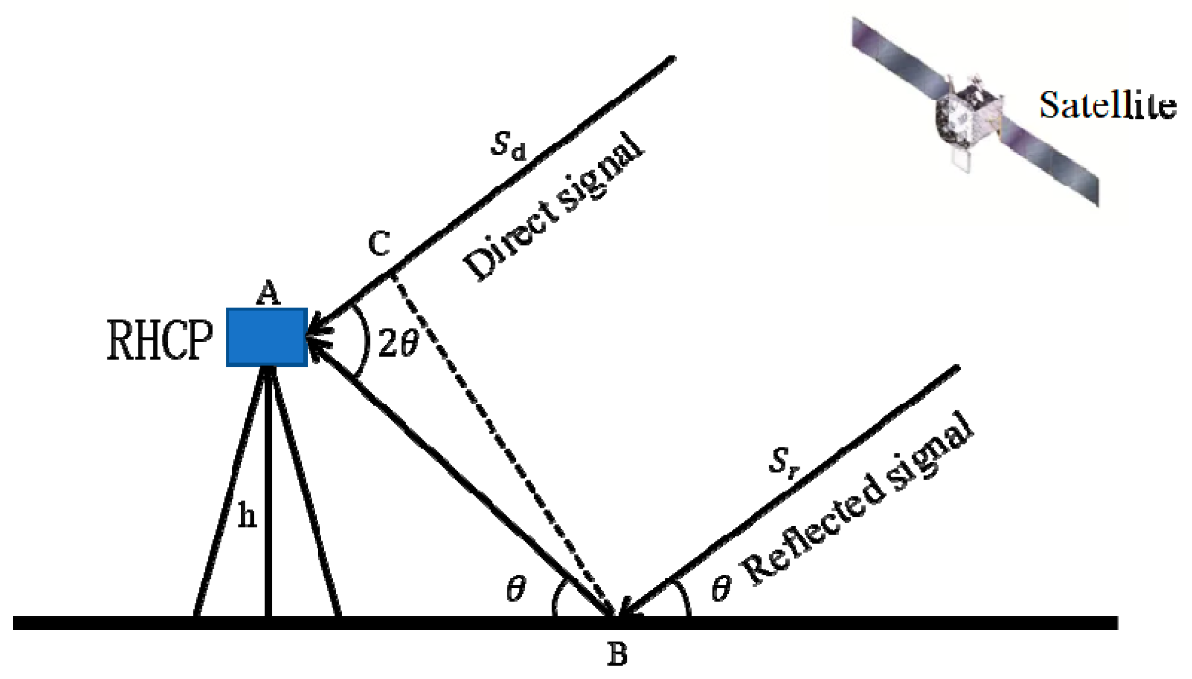
The microwave signal emitted by a GNSS satellite will inevitably produce a multipath effect in the process of propagation. The composite signal formed by the direct satellite signal (Sd) and the reflected satellite signal (Sr) that is reflected by the soil under the interference effect is received by the receiver. After processing, the composite signal data, namely SNR data, is generated. The basic principle of signal reflection is shown in Figure 1 [14]. RHCP is a right-handed circularly polarized antenna that can receive arbitrary polarized incoming waves, and its radiation wave can also be received by any polarized antenna. When the polarized wave is incident on a symmetrical target (such as a plane, sphere, etc.), the rotation direction is reversed, and the electromagnetic waves with different rotation directions have a large value of polarization isolation.
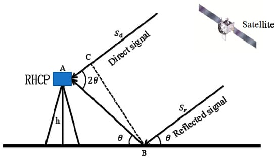
Figure 1.
GNSS signal reflection schematic.
SNR is mainly composed of the following two parts [28]:
where SNR is the composite signal that is formed after interference; SNRd is the SNR trend signal, namely the direct SNR signal; and dSNR is the residual sequence of SNR after removing the trend term, that is, the reflected SNR signal. From the point of view of signal oscillation, the SNR sequence can also be represented by the amplitude and phase difference of the oscillation [29]:
where the Ad is the oscillation amplitude of the direct signal component, Ar is the oscillation amplitude of the multipath reflection signal component, and is the phase difference between the two. During the motion of a satellite, the phase difference between the direct signal and the reflected signal changes with the variation of the satellite’s altitude angle , reflected in the enhancement and weakening of the SNR value affected by signal interference. Due to multipathing and antenna gain, the oscillation of SNR values is more pronounced at low altitude angles.
Due to the effective suppression of multipath signals reflected from the surface by the measurement type GNSS receiver antenna, the amplitude of the direct signal is much greater than that of the reflected signal, i.e., Ad >> Ar. This article decomposes and removes trend terms through wavelet analysis to eliminate Ad + Ar (oscillation amplitude of direct signal component and a small amount of multipath reflection signal component) in Formula (2). The remaining part can be approximated as a cosine model [30]:
where the dSNR is the residual sequence at low altitude angles containing reflection information, A is the amplitude, h is the antenna height, e is the satellite altitude angle, and φ is the relative delay phase of the reflected signal. Assuming , , then Equation (3) can be simplified as a standard cosine function expression [17]:
Perform LSP spectral analysis on the SNR residual sequence to obtain the oscillation frequency f, and then use the least squares fitting method to obtain the amplitude A and relative delay phase φ. Research has shown that there is a strong correlation between the characteristic parameters (frequency, amplitude, and phase) of satellite reflection signals and SM, which can be used for regression and inversion prediction of SM [14].
2.2. Wavelet Analysis Theory
In Formula (1), SNR contains the direct signal component and the reflected signal component. The trend term needs to be eliminated from the SNR sequence to obtain the dSNR residual sequence, and then the equivalent antenna height is obtained using LSP spectrum analysis. The commonly used method to eliminate the trend term is the second-order polynomial method. However, a large number of studies have shown that the wavelet analysis method is superior to the second-order polynomial method [29,31,32,33,34]. Therefore, the method of wavelet analysis [29] is adopted in this paper. The principle is as follows.
Let SNR observation G(t) be:
where t is the epoch. The algorithm of wavelet analysis is:
where Aj is the wavelet coefficient of low-frequency signal, j is the decomposition level, Dj is the wavelet coefficient of high-frequency signal, G(t) is the original signal, and t is the epoch. Using db4 as the wavelet basis (the wavelet basis function and the number of decomposition layers in this paper are determined by the integration of the literature [29,31,32,33,34] and the comparison of several commonly used wavelet basis functions. In view of its complexity, the repeated test process is not described in this paper), the original SNR sequence is decomposed into four layers. The original SNR signal is subtracted from the fourth layer of the low-frequency signal to eliminate the trend term and obtain the reflected signal.
2.3. Inversion of NDVI Based on Multi-Path Effects to Characterize Vegetation Effects
The microwave signal reflected by surface vegetation contains a large amount of VMC information [35], which significantly affects the SM inversion accuracy of GNSS-IR. Therefore, it is necessary to consider and remove the vegetation effect when using GNSS-IR to retrieve SM. Based on GPS pseudorange, carrier phase, frequency, and wavelength, Larson and Small (2014) proposed the normalized microwave reflectance index (NMRI) and mapped it to NDVI [9,19]. The multipath error of L1 carrier (MP1) can be expressed as [14]:
where MP1 is the multipath error of L1 carrier; P1 is the pseudorange observed by the L1 carrier; f1 and f2 are the frequencies of the L1 and L2 carriers, respectively; λ1 and λ2 are the wavelengths of the L1 and L2 carriers, respectively; and φ1 and φ2 are the phases of the observed L1 and L2 carriers, respectively [14].
Based on the epoch-varying MP1, the root mean square (RMS) of the MP1 of a single satellite per day is calculated. Subsequently, the RMS of MP1 per day is calculated using a weighted summation of the values observed by each satellite per day [36]. NMRI can be expressed as [14]:
where max(RMSMP1) is the average value of the largest 5% of the RMSMP1 values in the annual time series and RMSMP1 is the RMS of the MP1 of a single day. For the same period as that of the NDVI values, the NMRI values are obtained by down sampling the calculated values of the NMRI. In addition, the mapping model is employed to calculate the NDVI of the experimental period [14].
NDVI is a parameter reflecting vegetation growth conditions and vegetation coverage. The vegetation around the station is the main factor leading to the amplitude and phase offset of the reflected signal. The offset is the vegetation error of the GNSS-IR inversion SM, which needs to be eliminated before the inversion. In the absence of measured VMC data, NDVI is the main factor reflecting the amplitude and phase offset of the reflected signal [14].
2.4. Random Forest Model
The RF algorithm has advantages in data analysis and inversion and has been widely used in many fields, such as soil moisture and ecological environments. In the 1980s, Breiman et al. developed the classification tree method into an RF algorithm, which has a small amount of calculation and high accuracy. Through the integration idea, multiple decision trees are combined to solve the single inversion problem of the model. The basic idea is to randomize the initial data to generate a certain number of unrelated decision trees, and then calculate the final result using a weighted average of multiple decision trees according to different input variables. The advantages of this algorithm are as follows: (1) for a variety of input data, a high-accuracy analyzer can be generated that can process and analyze a large number of input variables; (2) it can automatically evaluate the importance of variables and generate corresponding weights. The advantages of RF can be summarized as the following: high parallelism of data, strong generalization ability of the constructed model, small variance, and insensitivity to the lack of data features. Considering that it is necessary to use NDVI data to eliminate the amplitude and phase offset caused by the vegetation effect from the amplitude and phase data obtained by GNSS-IR, the RF algorithm was employed to eliminate vegetation error for SM inversion by multi-GNSS and multi-frequency data. To verify the efficiency of the RF algorithm, two strategies, namely RF-After (RF-AF) and RF-Synchronous (RF-SY), were adopted and compared. For the RF-AF strategy, the NDVI data were first used to remove the influence of vegetation on the characteristic parameters of single-satellite and single-frequency GNSS signal, and then the RF algorithm was employed to fuse the filtered data. For the RF-SY strategy, the RF algorithm was used to process the characteristic parameters of multi-GNSS and multi-frequency signals by setting thresholds and optimizing parameters, and then the NDVI data were used to eliminate the influence of vegetation while fusing the characteristic parameters synchronously using the RF model to perform SM inversion and obtain a better signal combination for inversion.
3. Data Sources
3.1. GNSS Observations
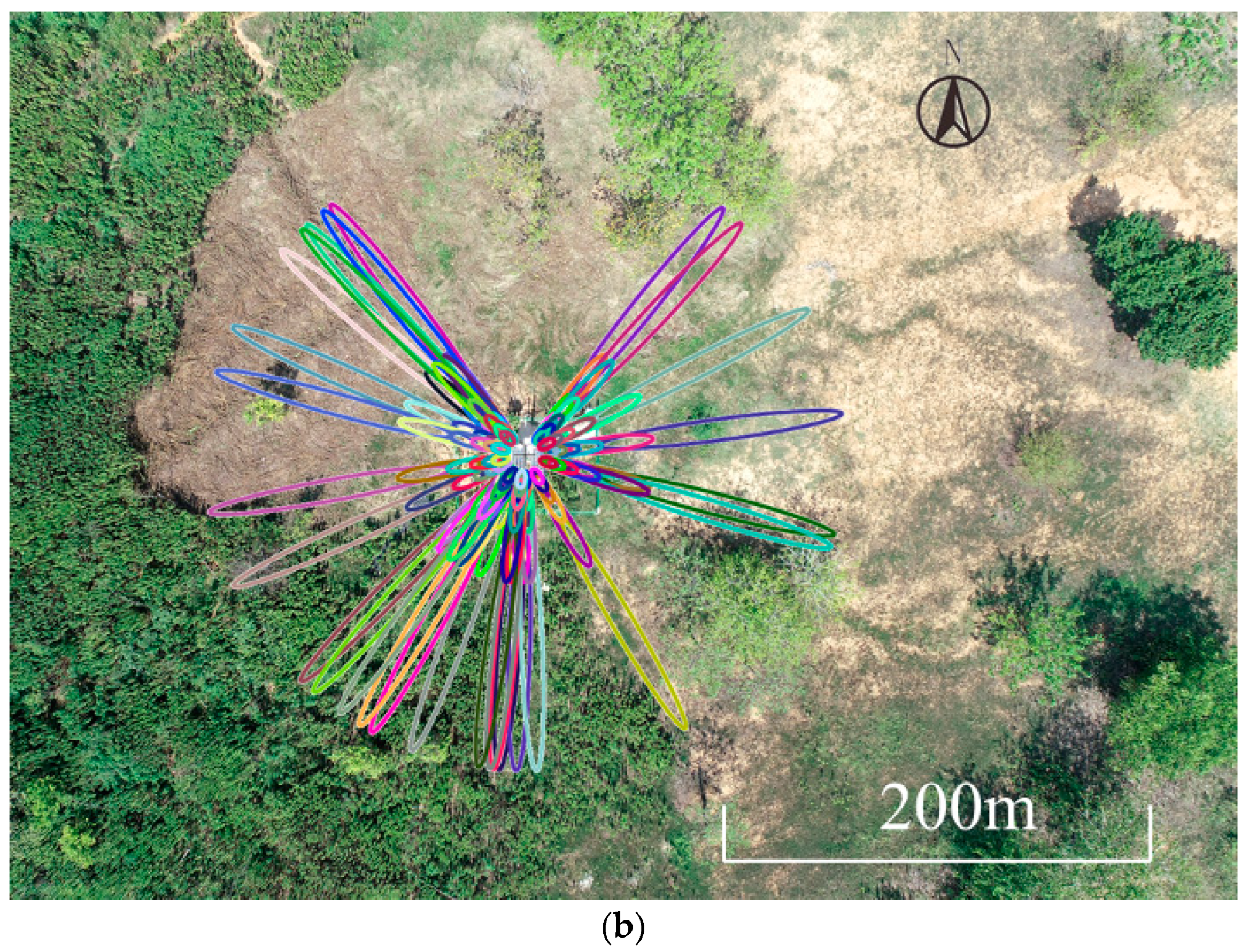
The experimental data were collected from the self-built Baima (NJBM) GNSS station (31.610647°N, 119.161229°W) seen in Figure 2. The station is located in Baima Town, Lishui District, Nanjing City, China. The height of the GNSS receiver is 4 m from the surface, with about a 150 m radius of the first Fresnel reflection zone [3]. This means observations of the NJBM station can be used to retrieve SM for an area within a 150 m radius. The receiver model of NJBM is shown in Table 1. The four seasons of the station are clear, hot, humid, and rainy in the summer and cold and dry in the winter. The average annual temperature is 16.1 °C, the average annual relative humidity is 76%, and the average annual precipitation is 1204.3 mm. The terrain of the area is gentle, and the north and east of the NJBM site consist of bared soil, with the south and west vegetated mainly by Canada Goldenrod. The warm and rainy climatic conditions and the surface conditions around the station are helpful in verifying the feasibility of ground-based GNSS-IR technology in SM inversion accounting for vegetation effects. GNSS observation data of NJBM Station for 171 days from 9 July to 31 December 2022, i.e., day of year (DOY) 190–365, 2022, were collected. The precise ephemeris SP3 data corresponding to DOY were downloaded, and Python was used to extract the epoch, elevation angle, azimuth angle, and SNR data of each frequency band of GPS and BDS satellites required for the experiment.
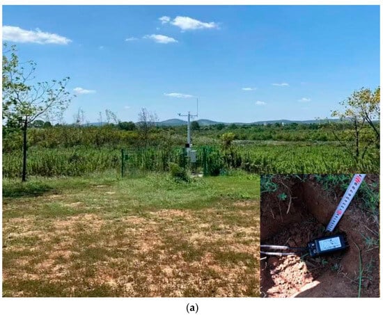
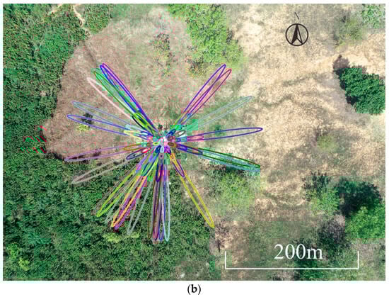
Figure 2.
Surrounding environment and experimental equipment. (a) Real time photo of Baima Station (taken from the east side of the station in 2022) with an SM sensor buried at a depth of 5 cm. (b) Distributions of the first Fresnel reflection zone. The elliptical coverage area from small to large represents the reflection zone of 5°, 10°, 15°, and 30°, respectively.

Table 1.
The receiver of NJBM station and its related parameters.
3.2. NDVI
The NDVI data were obtained by analyzing and calculating the Sentinel-2 satellite images during the studying period through the Google Earth Engine platform. The spatial resolution of the data was 10 m and the temporal resolution was 7 days. Since the time resolution of GNSS-IR was 1 day, to match the data, it was necessary to use the strong correlation between NMRI and NDVI calculated by a GNSS multipath to retrieve the NDVI data with a time resolution of 1 day.
3.3. Auxiliary Data
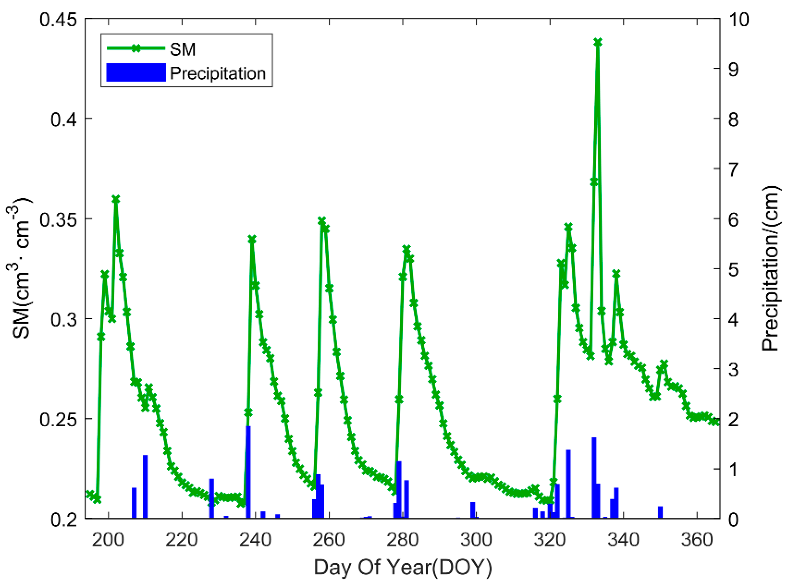
The NJBM station also monitored the precipitation with a co-located rainfall sensor, as well as in situ SM values with a co-located SM sensor on a time scale of 0.5 h, and the average value was taken as daily values after a data quality test.
Figure 3 shows the SM and precipitation data series observed by DOY 195–365 in 2022, represented by line charts and histograms, respectively. As shown in Figure 3, there were nine significant precipitation events during the experiment, with a maximum precipitation of 21.4 mm. During precipitation events, SM increased significantly, especially in DOY 207–210, 238–242, 256–258, 278–281, 310–325, and 332–338. Continuous precipitation led to a significant nonlinear increase in SM. With the decrease or cessation of precipitation, the content of SM also decreased. Obviously, precipitation is the main factor leading to the sudden change of SM. It is indicated that the environment and the meteorological condition of the NJBM site are suitable for SM inversion.
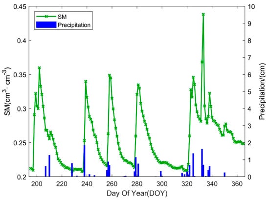
Figure 3.
The in situ SM and rainfall diagram during the experimental period.
4. Experiment and Results
4.1. SM Retrieval Strategy
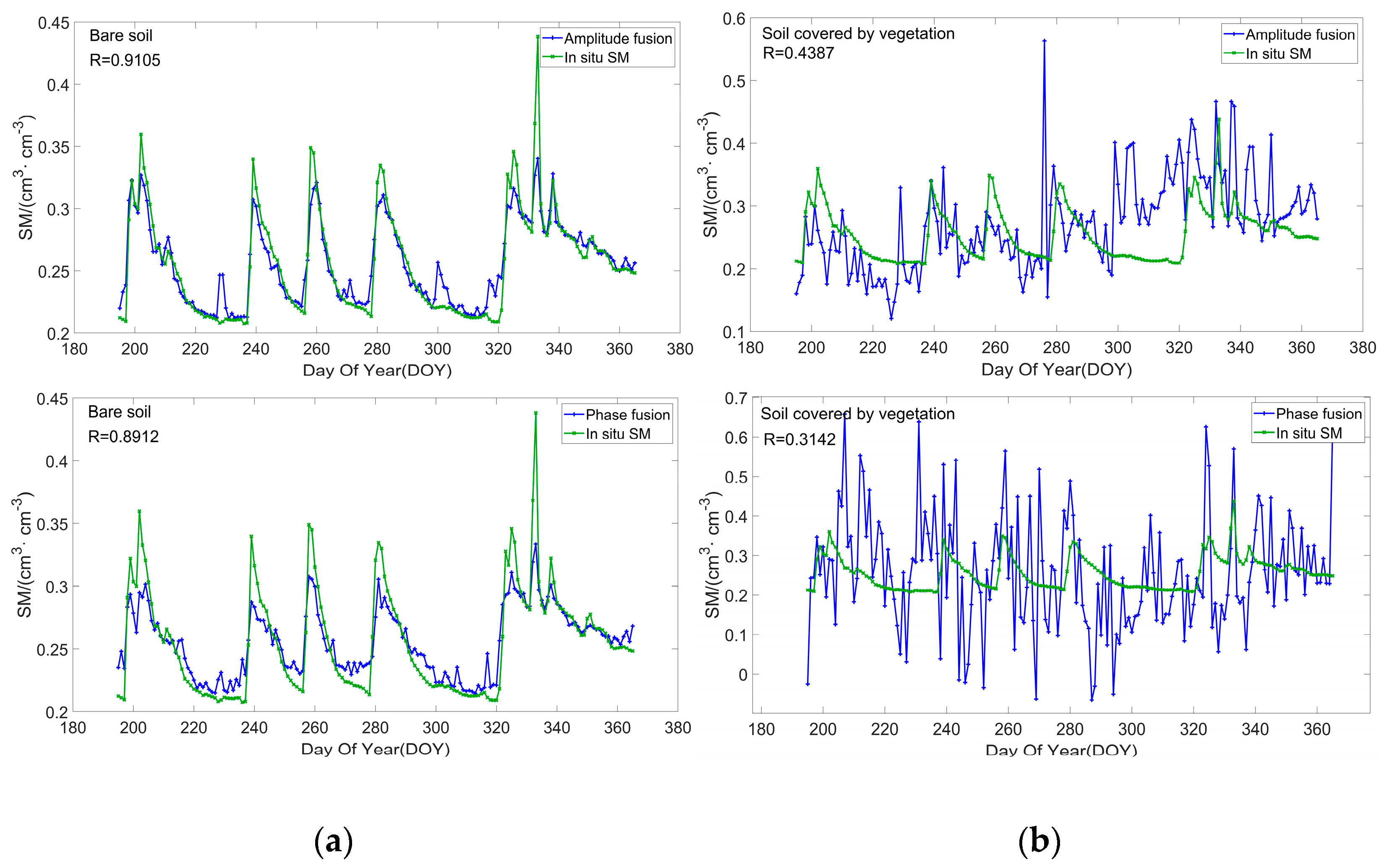
It can be seen from Figure 2 that the northern part of the NJBM station is a bare soil area without vegetation coverage, and the azimuth range is −90°–90°. The receiver can directly receive the GNSS signal reflected by the surface soil, so the traditional GNSS-IR method can be used to retrieve the soil moisture, including the following three steps: Firstly, the GNSS observation files, precise ephemeris, and soil moisture measured data of the study period are downloaded, and the GNSS elevation angle, azimuth angle, epoch, and SNR data are obtained through data preprocessing. Secondly, the SNR signal data with an elevation angle of 0–30° and an azimuth angle of −90–90° are screened. The direct signal in the SNR is decomposed and eliminated by wavelet analysis, and the reflected signal representing the physical parameters of the surface soil is retained. The frequency, amplitude, and phase characteristic parameters of the SNR-reflected signal are obtained with LSP spectrum analysis and the least square method. Finally, the random forest algorithm is used to retrieve the SM derived from the amplitude and phase, respectively, and compared with the in situ SM observations. Due to the fact that the limitation of space and the bare soil part are not the main research area of this paper, the specific steps can be referred to the reference [29], and the SM inversion results are shown in Figure 4a. At the same time, the southeastern part of the survey area is a light vegetation coverage area, and the southwestern part is a vegetation coverage area. In order to better analyze and study the impact of vegetation on GNSS-IR SM inversion, the southwestern part of the station is selected as the study area, and the azimuth angle is 180–270°. The soil moisture inversion results of the region using the above steps are shown in Figure 4b.
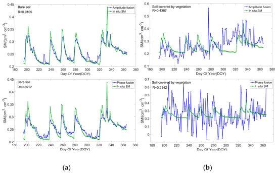
Figure 4.
Inversion results of soil moisture. (a) Inversion results of amplitude and phase fusion in the bare soil area. (b) Inversion results of amplitude and phase fusion in vegetation coverage areas.
From Figure 4, it can be seen that the SM retrievals derived from amplitude or phase through traditional methods are consistent with the in situ SM observations in the bare soil region. However, the SM inversion effected in the vegetation-covered area under the same steps is not ideal. This is because the moisture in the vegetation-covered area also reflects satellite signals to the receiver, which not only receives direct GNSS signals and reflected GNSS signals from the soil through the vegetation, but also receives GNSS reflection signals from the vegetation. This makes the extracted SNR signal feature parameters inaccurate due to the influence of vegetation, resulting in poor inversion results. Therefore, for soil moisture inversion in vegetation-covered areas, the error caused by vegetation impact should be eliminated after extracting feature parameters. At the same time, in the absence of measured VMC, NDVI values in vegetation-covered areas can be used to characterize vegetation impact.
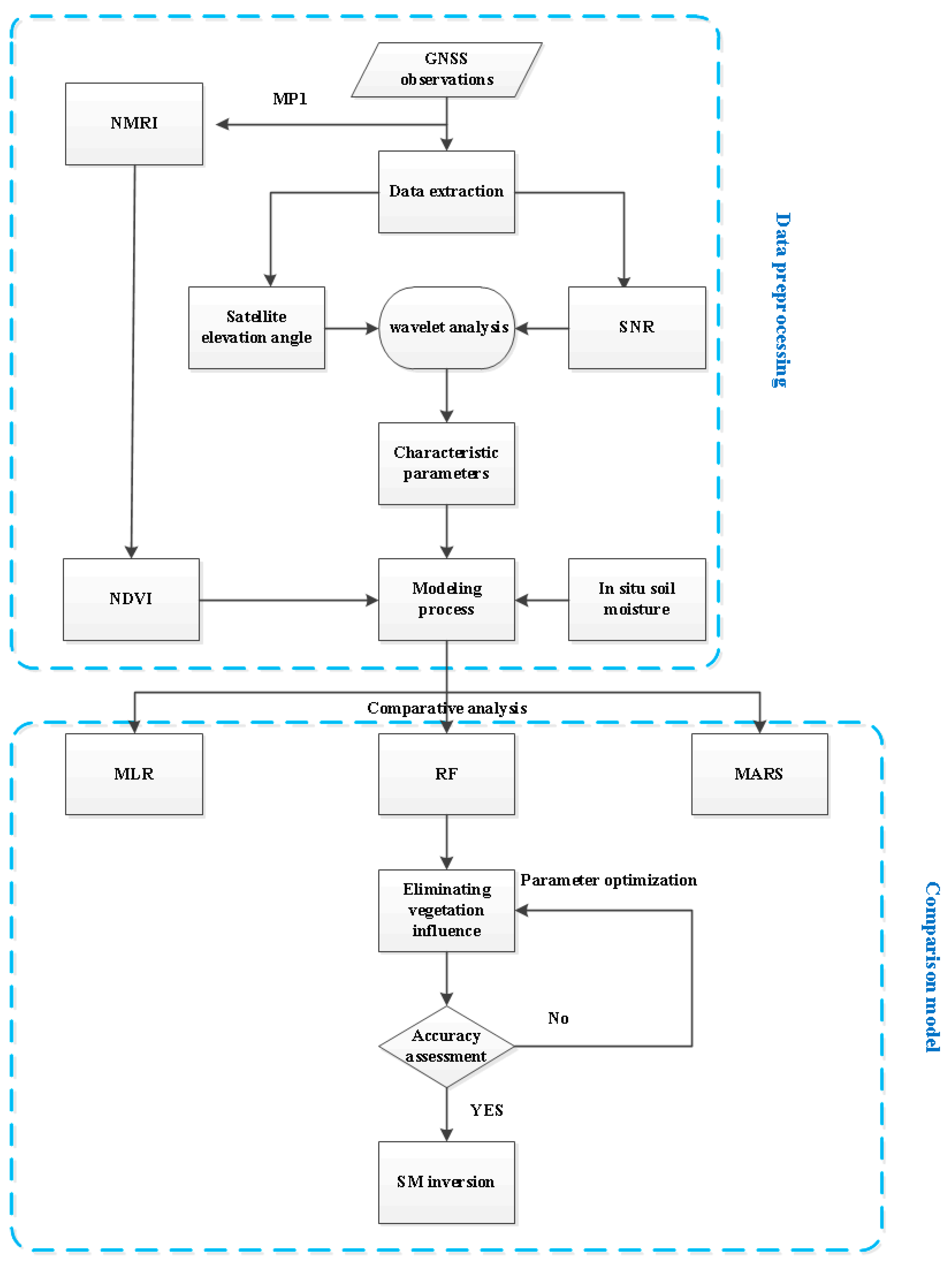
Based on the above comparative analysis experiments, Figure 5 shows the flow chart of the SM inversion strategy proposed in this study. Firstly, the characteristic parameters with the amplitude and phase of the reflected signals from the SNR data extracted from GNSS observations were calculated. At the same time, NMRI was calculated using multipath data from GNSS observations, and it verified the correlations between NMRI and NDVI on a 7-day scale. On this basis, an NMRI–NDVI empirical model was established, and the NDVI with a 1-day scale that can characterize the impact of vegetation was performed using NMRI with a 1-day scale. Finally, SM was retrieved using the RF model to fuse the multi-GNSS and multi-frequency data with the influence of correcting vegetation effects, and it was compared to the traditional machine learning models of MLR and MARS.
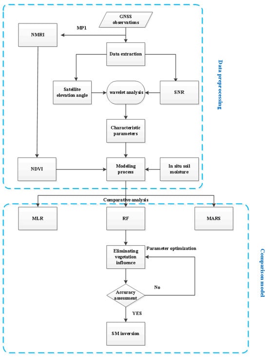
Figure 5.
Technical process of GNSS-IR SM inversion.
The machine learning algorithm is used in the current SM inversion model to improve the accuracy of the inversion process. However, due to the characteristics of the black box of machine learning algorithms, the parameters of the model are difficult to adjust. The proposed RF SM inversion model adaptively integrates multi-frequency and multi-GNSS data to improve vegetation error and selects the best satellite combination for SM inversion by changing parameters, resulting in high-precision inversion results. The GNSS-IR SM inversion model can be expressed by Formula (10):
where SM is the inversion result of SM, Gi is the machine learning model for regression inversion, and represents the input feature matrix after data normalization and characteristic parameter screening. , , and , represent the phase, amplitude, and frequency characteristic parameter sequences, respectively, and n1 and n2 are the corresponding characteristic parameter sequence entries.
4.2. Reflected Signal Feature Parameter Extraction
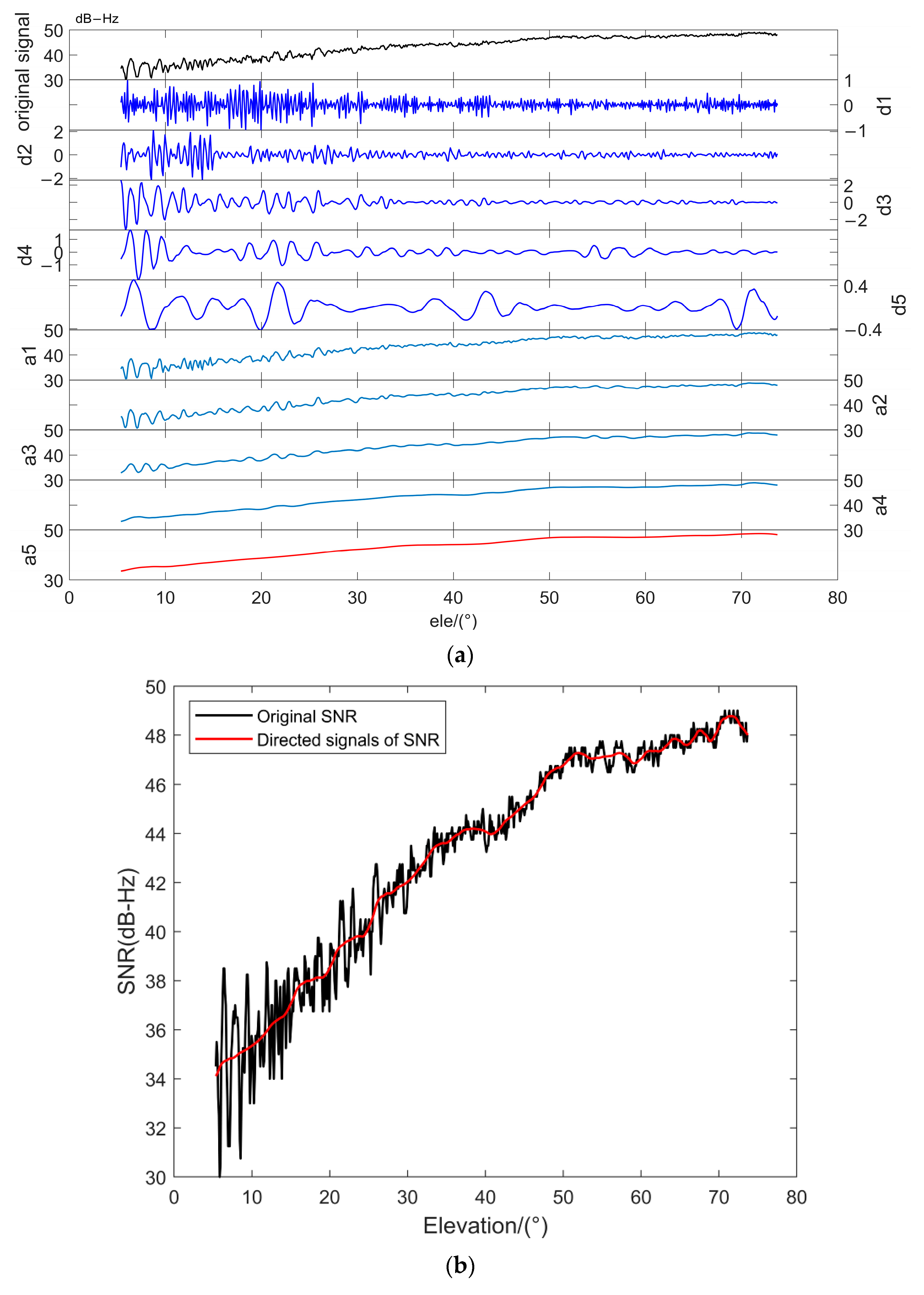
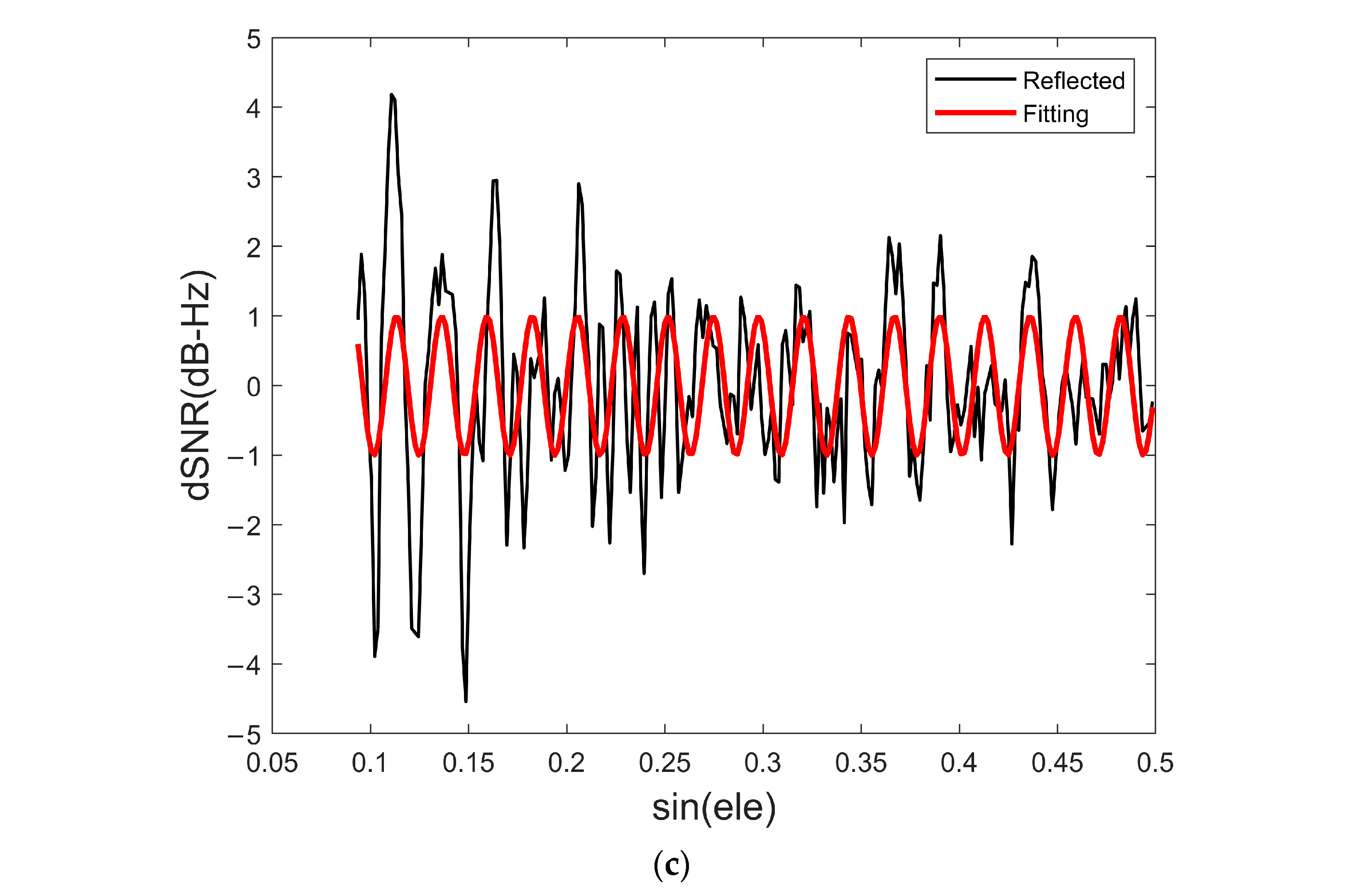
GNSS-IR SM inversion needs to use the GPS and BDS satellite elevation angle, satellite azimuth angle, and SNR data. For NMRI calculating, the observations of the carrier phase, pseudorange, frequency, and wavelength of GPS L1 are required, which are derived from GNSS observation files and navigation messages. The SNR data of G26 S1C (DOY 350) are taken as an example. To extract the reflected signal data from the GNSS SNR observations, the direct signal is separated from the SNR sequence using the wavelet analysis method, fitting the SNR residual sequence of the experimental area data using the cosine model (as seen in Figure 6).
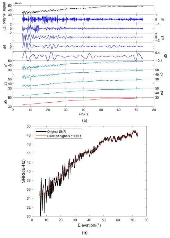
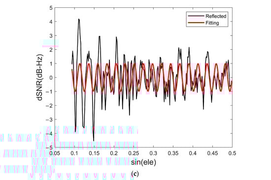
Figure 6.
GNSS SNR observation data processing. (a) Wavelet analysis results figure. (b) Direct signal extraction. G26 S1C SNR data (DOY 350) are shown in black. The direct signal is represented by the smooth curve in red. (c) The fitting curve of dSNR residual sequence and cosine model.
Figure 6a shows the results of the five-layer wavelet decomposition of the above SNR sequence using db4 as the wavelet basis. Among them, the black line is the original SNR sequence, and the dark blue line is a five-layer high-frequency signal decomposed by wavelet, that is, the detail signal, reflecting the detailed information of the original SNR sequence. The light blue line and the red line are the five-layer low-frequency signals under wavelet decomposition, also known as approximation signals, which are the slowly changing parts of the original SNR sequence. The red line is the trend term, that is, the direct signal. The relationship between the extracted direct signal and the original SNR signal is shown in Figure 6b. The SNR series is displayed in black, and the direct signal is displayed in red. At low satellite elevation angles, the SNR shows serious multipath effects and exhibits periodic oscillations. With the gradual increase of the satellite elevation angle, the antenna gain is considerable, and the SNR is stable. Therefore, the elevation angle range of this experiment is set to 5~30°. The vegetation coverage area is selected with an azimuth range of 180~270° according to Figure 2b. By subtracting the trend term from the original SNR sequence, the SNR residual sequence can be retained. The frequency f can be obtained by LSP spectrum analysis, and the amplitude A and phase φ can be obtained by fitting the SNR residual sequence with the cosine model of the least square method. The results are shown in Figure 6c.
4.3. Inversion of NDVI Representing Vegetation Effect
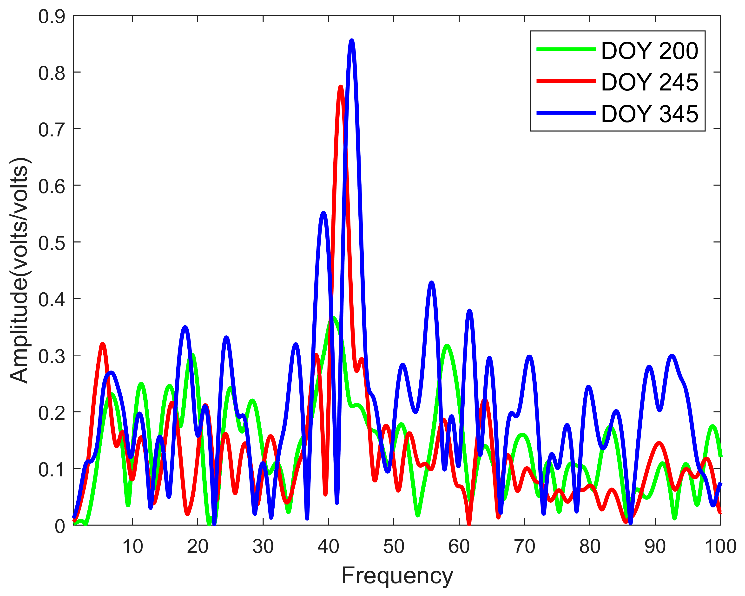
When using GNSS-IR to retrieve SM, the change of vegetation will correspond to the increasing or decreasing of the amplitude and phase shift of the reflected signals. Therefore, it is necessary to correct the influence of vegetation. Figure 6 shows the power of the reflected signals through LSP spectrum analysis on DOY 200, 245, and 335. It can be seen that there are obvious variations of the power on different days that are mainly due to the different conditions of the vegetation. In the absence of measured VMC, NDVI data can be used to characterize the impact of vegetation [14]. Since the temporal resolution of the NDVI data is 7 days, it cannot be used to eliminate the daily vegetation effect to retrieve the SM. Meanwhile, through Formulas (8) and (9), the GNSS observation data can be used to calculate the NMRI with a 1-day temporal scale, and the strong correlation between NMRI and NDVI can be used to establish a linear regression model to retrieve the NDVI [14]. To solve the reflected signal changes caused by different vegetation conditions, the established NMRI–NDVI correlation model was used to retrieve the NDVI data that can characterize the vegetation effect.
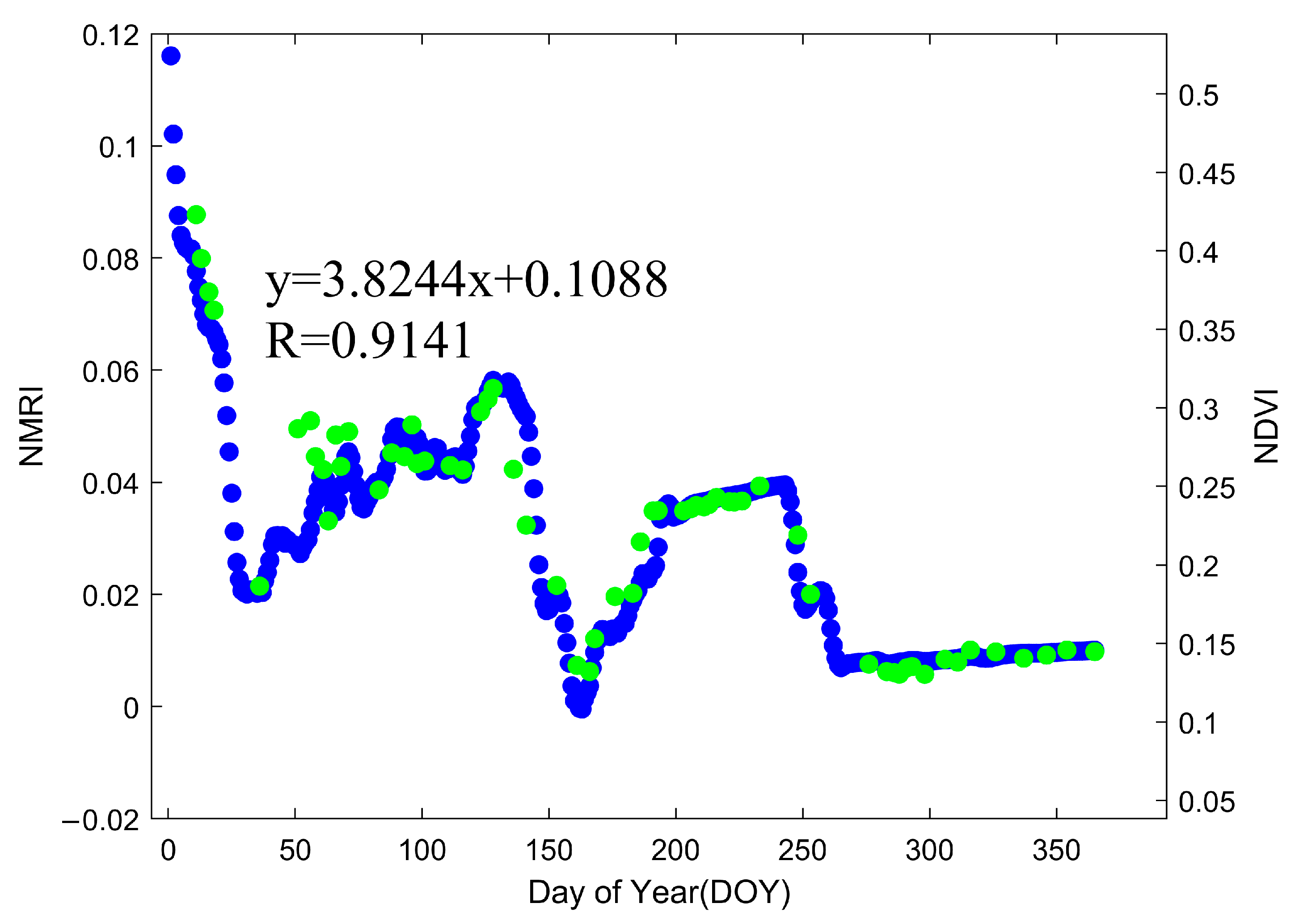
The vegetation in the experimental area is mainly Canada Goldenrod, with some evergreen trees and a few experimental shrubs sporadically distributed. As in Section 3.1, the unique growth characteristics of Canada Goldenrod and two mowing actions (DOY 1~25 and DOY 245~260) affect the NDVI series. At this time, It can be seen in Figure 7 that when the vegetation around the site is in a vigorous stage (DOY 200), the amplitude of the reflected signal is the smallest, while the amplitude begins to increase in the mowing action (DOY 245), leading to the maximum after Canada Goldenrod removal (DOY 335). Affected by the vegetation growth cycle, the dominant frequency of each DOY has a corresponding increase or decrease. Figure 8 shows the distribution of 1-day NMRI values and 7-day NDVI values during 2022. From the figure, it can be seen that the NMRI calculated by GNSS multipath data also changes with the different growth conditions of vegetation in the time series, and its fluctuation trend tends to be consistent with NDVI in the time domain. In addition, the trends and directions of NMRI are also well-matched with NDVI. The 7-day NMRI values were extracted corresponding to the DOY of NDVI. Then, a simple linear regression model between the NMRI and the NDVI was established:
where y is the inversion NDVI, and x is the NMRI with a time scale of 1 day. This finding indicates that NDVI can characterize vegetation growth, and that there is a strong linear relationship between NMRI and NDVI with R of 0.9141, and NDVI data can be retrieved in a time scale of 1 day.

Figure 7.
L-S spectrum analysis at the corresponding time.
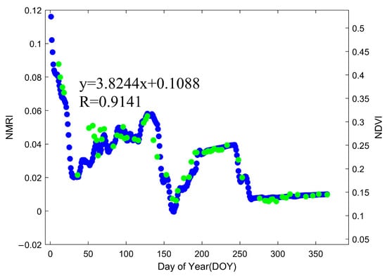
Figure 8.
The NMRI–NDVI time series of 2022.
4.4. SM Retrieval Experiment and Results
The RF-AF strategy is established to correct the characteristic parameter offset for the GNSS signal data of different frequency bands, as well as of different satellites, and then input the filtered available data into machine learning models, such as RF for fusion inversion [14]. Although the RF-AF strategy can eliminate the influence of vegetation on the inversion of SM, due to the different systematic errors between different frequency bands and the different trajectories between different satellites, the vegetation effects were different. Therefore, it is necessary to establish correction models for the A and P of each satellite based on the RF-AF strategy. Considering that the models were different, it would lead to poor universality, gross errors, and low efficiency. The experiment in Figure 4 shows that the amplitude and phase of satellite SNR signals are strongly correlated with SM, and NDVI can characterize the vegetation effect [22]. Therefore, they are the main data for inverting SM in vegetation coverage areas. The RF-SY strategy proposed in this paper uses amplitude and phase data, as well as the NDVI as the input data. The algorithm and modeling process are as follows:
Train and establish the model by inputting data from the first 100 days into the RF model, and set the initial parameters and initial thresholds of the algorithm (R > 0). Because the influence of vegetation on GNSS-IR technology is mainly reflected in the amplitude and phase offset, it will not excessively affect their overall trends [14,15]. After the verification of the bare soil area, the SM inversion value of GNSS-IR has a strong positive correlation with the in situ SM value [12]. Therefore, the initial threshold can be set to R > 0, and satellites with correlation coefficients less than 0 can be considered unavailable and removed. During the operation of the RF model, the inversion accuracy requirement is set to a correlation coefficient of ≥0.8. If the inversion accuracy does not meet the accuracy requirements, the parameters and thresholds will be automatically adjusted (considering the utilization of satellite data, the maximum threshold is R > 0.5, and the threshold adjustment scale is 0.1) and rebuilt. If the inversion accuracy meets the accuracy requirements, visualize and record the model parameters, inversion results, and inversion accuracy. Continue adjusting the parameters while keeping the threshold constant. If the inversion accuracy meets the accuracy requirements ten consecutive times, the model with the highest inversion accuracy recorded in the loop output will be skipped. During the parameter adjustment process, the number of decision tree models included in the random forest model, the maximum number of features selected to construct the decision tree, and the maximum number of selected features will randomly increase or decrease in a ratio of less than or equal to 5. The maximum depth of the decision tree model and the minimum number of samples for leaf nodes remain unchanged, while the minimum number of samples allowed to split at the current node remains unchanged until better satellite combination inversion results are obtained. This achieves the effect of eliminating vegetation impact while achieving data fusion, as shown in Table 2 and Table 3. The final selected model parameters are shown in Table 4 (taking RF-SY amplitude inversion as an example). Finally, input the amplitude, phase, and NDVI data of DOY 190−365—the optimal satellite combination output during the modeling process, into the established model for SM inversion—and compare it with the in situ SM.
Table 2.
The signal frequency band and the corresponding satellite number used to process the best combination of amplitude data.
Table 3.
The signal frequency band and the corresponding satellite number used to process the best combination of phase data.
Table 4.
Final selected model parameters.
To test the feasibility and effectiveness of the RF model, and considering that the machine learning algorithm has a self-learning and adaptive ability to solve high-dimensional nonlinear problems, three schemes were developed for comparative analysis. Specifically, Schemes 1 and 2 are the comparison of the proposed RF-SY strategy and RF-AF strategy, respectively. Schemes 1, 2, and 3 involve the RF inversion model based on multi-satellite fusion, the MARS inversion model based on multi-satellite fusion [14], and the MLR inversion model based on multi-satellite fusion [14].
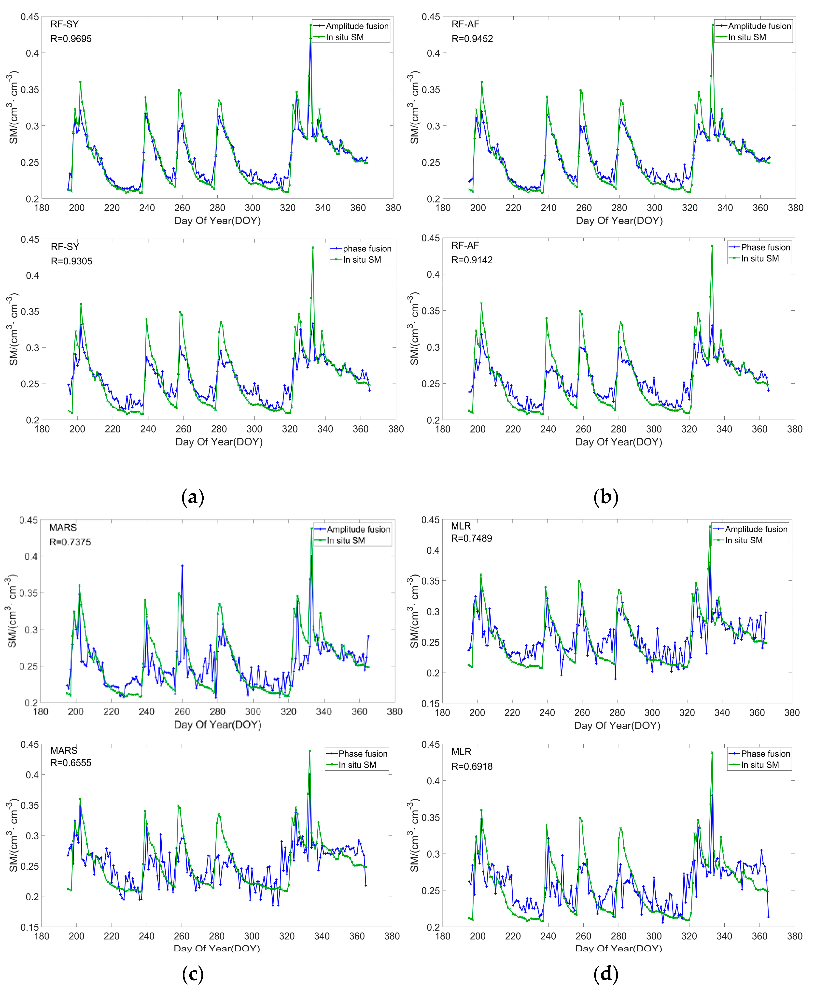
Figure 9 shows the validation of the SM retrievals and the measured in situ SM of the three models, as well as the accuracy comparison with the RF-AF (the blue line and the green line represent the retrieved SM value and the measured SM value, respectively).
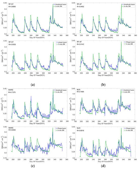
Figure 9.
(a) RF-SY fusion correction amplitude, phase two characteristic parameters of SM comparison diagram. (b) RF-AF fusion correction amplitude, phase two characteristic parameters of SM comparison diagram. (c) MARS fusion correction amplitude, phase two characteristic parameters of SM comparison map. (d) SM comparison of MLR fusion correction amplitude and phase two characteristic parameters.
Comparing Figure 9a,b, it can be seen that both the RF-SY strategy and the RF-AF strategy can retrieve relatively highly accurate SM. However, the SM time series curve retrieved by the RF-SY strategy is smoother than the RF-AF strategy with less fluctuation. By comparing Figure 9a,c,d, it can be found that although the SM retrieved by the traditional MLR and MARS models is consistent with the measured in situ SM change trend to a certain extent, there is still a large fluctuation. It can only retrieve the overall change trend of SM, and the reliability of its specific value is poor. The RF model can more satisfactorily retrieve the trend of the SM, the estimation error is more stable, the fluctuation is smaller, and the reliability of the inversion value is higher. This model effectively improves the problem of the low SM inversion accuracy of MLR and MARS models. In addition, in the absence of vegetation correction, each retrieved SM using the four models showed some fluctuations. Meanwhile, without vegetation correction, the average correlation coefficient of single satellite data inversion in the better satellite combination is only 0.374, while the inversion correlation coefficients of the two RF models (RF-AF and RF-SY) and two traditional models (MARS and MLR) are all greater than 0.65. This shows that the amplitude or phase shift inversion using machine learning models to correct the influence of vegetation in the characteristic parameter data is much more accurate than the inversion using the original characteristic parameter data. This finding further proves the feasibility of correcting the vegetation effect when using GNSS-IR to retrieve SM.
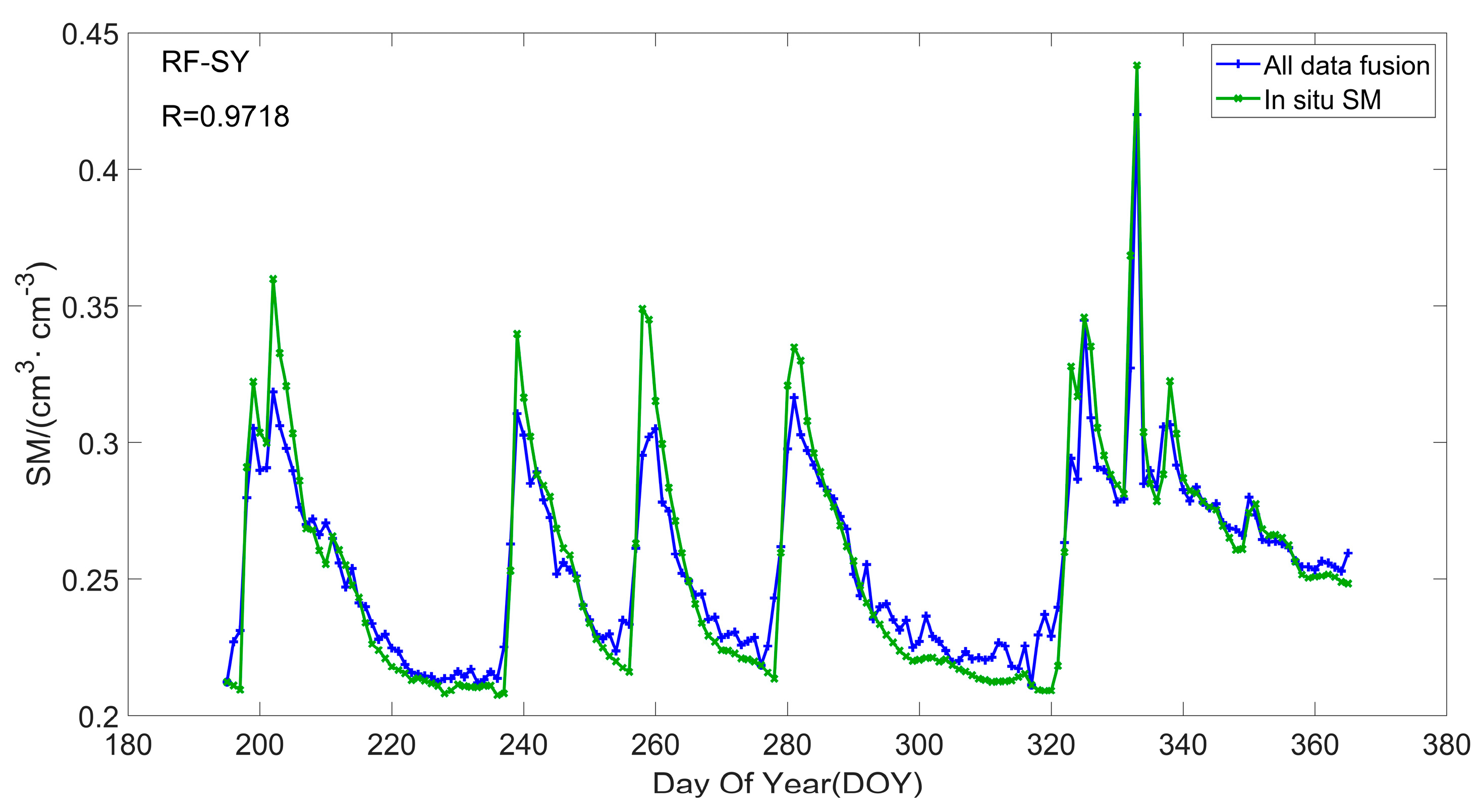
Meanwhile, from Figure 9a, it can be found that the RF-SY amplitude fusion correction model can better respond to the SM change caused by precipitation, and the RF-SY phase fusion correction model has higher local accuracy than amplitude fusion in some DOY with R of 0.9695 and 0.9305, respectively. Therefore, the RF model is suitable to be used to fuse the amplitude and phase data, and the results are shown in Figure 10.
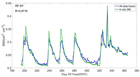
Figure 10.
Inversion results of amplitude and phase fusion correction model based on RF-SY algorithm.
From Figure 10, it can be seen that compared to the fusion correction of single feature parameters, the inversion results of simultaneous amplitude and phase fusion correction are better. The SM inversion sequence has a highly similar trend to the measured SM sequence in the overall part, and some inversion errors are eliminated in the details, resulting in a significant improvement in the entire inversion result.
5. Discussion
SM Inversion Correlation Analysis
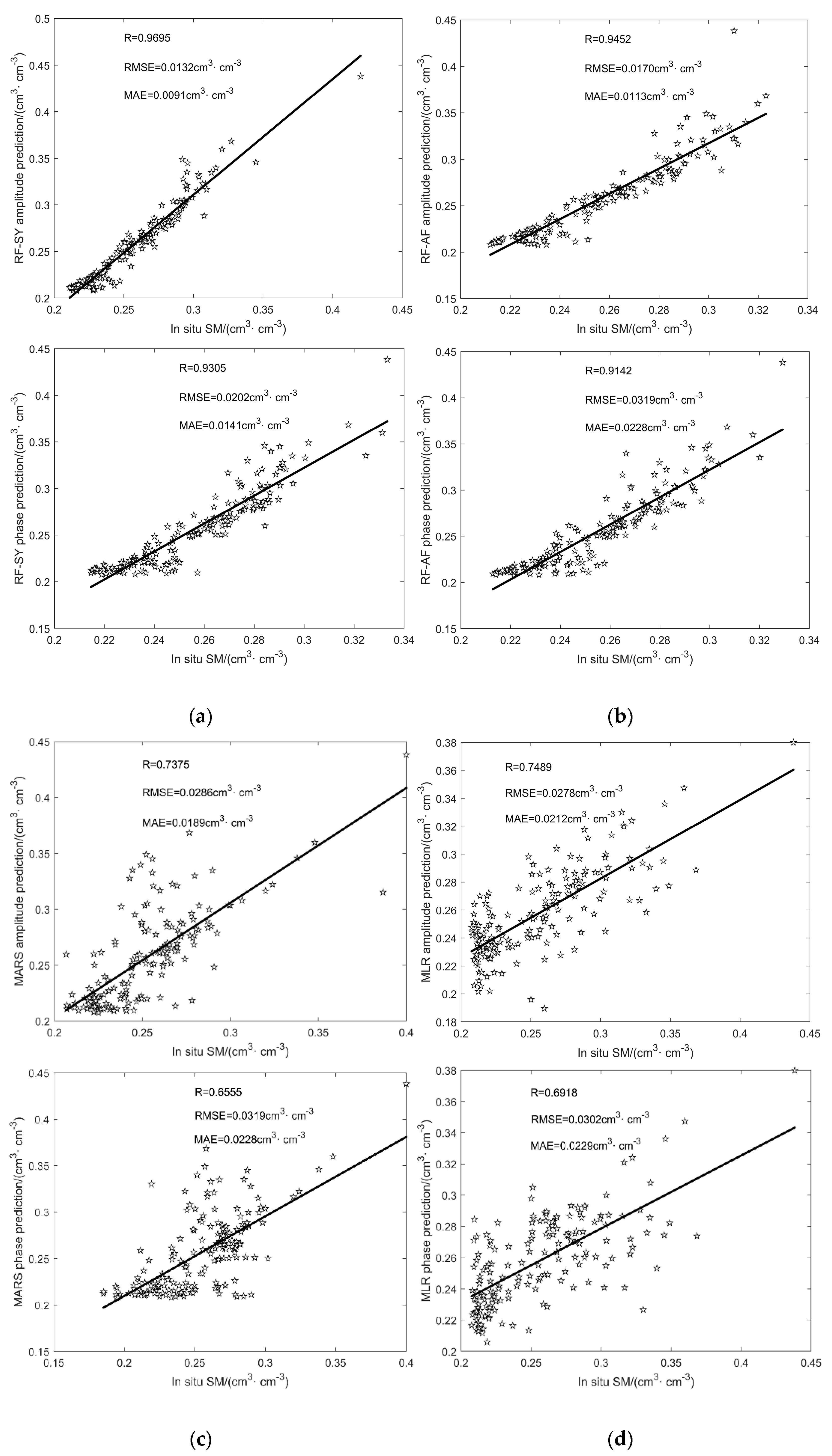
Considering Figure 7 and Figure 8, the calculated NMRI of the NJBM station is well related to NDVI. Figure 9 verifies the accuracy and reliability of the vegetation correction methods mentioned above. The correlation diagrams of the results obtained by the four models verify the feasibility and accuracy of the proposed RF model. The results show that the correlation of the four models is increased by at least 52.4% by correcting the vegetation effect. This result shows that the NMRI derived from GNSS multipath signals can be used to effectively correct the amplitude and phase errors caused by vegetation effects. Figure 11 shows the scatter plots of the inversion SM and the measured SM corresponding to each method in Figure 9, from which the inversion effect can be more intuitively and finely observed.
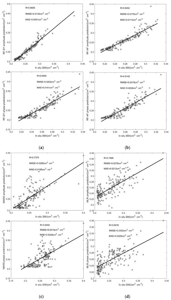
Figure 11.
(a) Linear regression analysis of RF-SY inversion SM with corrected amplitude and corrected phase and measured SM. (b) Linear regression analysis of RF-AF inversion SM with corrected amplitude and corrected phase and measured SM. (c) Linear regression analysis of corrected amplitude and corrected phase MARS inversion SM and measured SM. (d) Linear regression analysis of corrected amplitude and corrected phase MLR inversion SM and measured SM.
To further comprehensively evaluate the performance of each scheme and verify the reliability and generalizability of the RF model proposed in this paper, the correlation coefficient R, root mean square error (RMSE), and mean absolute error (MAE) were used for accuracy evaluation. Figure 9 shows the R-value between the inversion SM and in situ SM based on four methods. Table 5 shows the accuracy indexes of the four methods.
Table 5.
Statistics of SM inversion accuracy of each model.
From the statistical results of Table 5, it can be seen that the proposed RF-SY strategy has a significant improvement in inversion accuracy relative to the proposed RF-AF strategy, whether for amplitude fusion or phase fusion. The R of amplitude fusion is increased by 2.6%, with RMSE reduced by 22.4% and MAE by 19.5%. Meanwhile, the R of phase fusion is increased by 1.8%, with RMSE reduced by 4.3% and MAE by 4.7%, which also directly proves that the proposed RF-SY strategy is better than the RF-AF strategy. While having better inversion accuracy, it reduces the time spent on multiple vegetation corrections and greatly improves the inversion efficiency. For amplitude fusion, The R values of the RF, MARS, and MLR models are 0.9695, 0.7375, and 0.7375, respectively. The RMSE values are 0.0132 cm3·cm−3, 0.0286 cm3·cm−3, and 0.0278 cm3·cm−3, respectively. The MAE values are 0.0091 cm3·cm−3, 0.0113 cm3·cm−3, and 0.0189 cm3·cm−3, respectively. For phase fusion, the R values of the RF, MARS, and MLR models are 0.9305, 0.6555, and 0.6918, respectively. The RMSE values are 0.0202 cm3·cm−3, 0.0319 cm3·cm−3, and 0.0302 cm3·cm−3, respectively. The MAE values are 0.0141 cm3·cm−3, 0.0228 cm3·cm−3, and 0.0229 cm3·cm−3, respectively. From Table 1, Table 2, Table 3, Figure 8 and Figure 9, it is suggested that for the fusion data selection, the SM retrieved from the amplitude data of reflected signals is better than that from the phase data, which means that the inversion accuracy of amplitude fusion is better than that of phase fusion, and the amount of amplitude data is larger and the data utilization rate is higher. For the selection of fusion models, all three machine learning models can effectively improve the unreliability and instability of single-satellite inversion and improve the accuracy of GNSS-IR SM inversion. Among them, the inversion accuracies of the MARS and MLR models are comparable, while the inversion accuracy of the RF model is much higher than those of traditional MARS and MLR models. Therefore, the RF fusion correction model based on integrated multi-frequency and multi-GNSS data ensures the local error stability in the inversion process, eliminates the satellite data that do not meet the quality requirements through the threshold and parameter cycle process, and obtains the optimal satellite combination for SM inversion. Compared to the conventional method, the RF model can suppress the gross error caused by single satellite data more effectively.
Aiming at the amplitude fusion analysis of SM inversion error, the absolute inversion error of SM (the difference between the inversion SM and the in situ SM, as shown in Figure 12) is calculated, and the interval distribution pattern is analyzed. Figure 12 is the statistical histogram of the absolute error ratio of SM inversion obtained by four methods. It can be seen that compared to in situ SM values, there is a large proportion of small absolute error in retrieved SM by all four models. The absolute error distribution of the RF model is in the range of 0.03~0.04, which is narrower than the error distribution of the other three methods, and generally conforms to the normal distribution. The results further illustrate the advantages of the RF-SY strategy for high-precision SM inversion, and the inversion result is better than the RF-AF strategy.
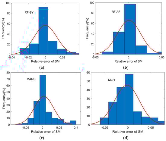
Figure 12.
(a) Statistical results of the relative error of RF-SY. (b) Statistical results of the relative error of RF-AF. (c) Statistical results of the relative error of MARS. (d) Statistical results of the relative error of MLR.
Since the RF fusion correction model is based on the integrated multi-frequency and multi-GNSS data, it can well adapt to the changes in vegetation growth from multi-reflected signals. Under the same conditions, the RF model shows better performance than the traditional MLR and MARS models, and the proposed RF-SY strategy is superior to the proposed RF-AF strategy.
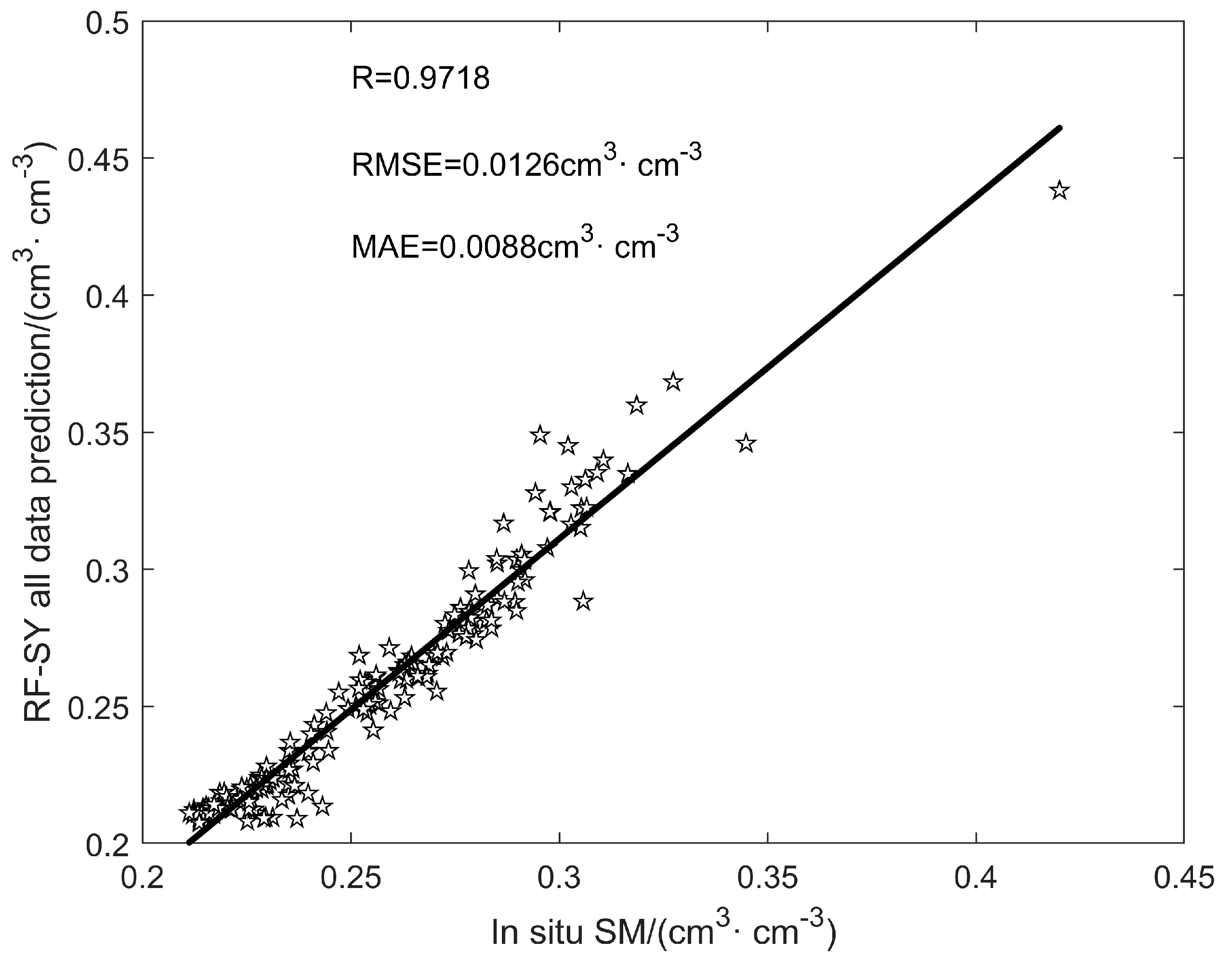
On the basis of the fusion correction results of single feature parameters, further discussion and evaluation are conducted on the inversion results of simultaneous amplitude and phase fusion correction, as shown in Figure 13 and Table 6. From the statistical results of Table 4, the amplitude and phase feature parameter fusion correction model based on RF can slightly improve the inversion accuracy of SM, the R is increased by 0.2%, the RMSE is reduced by 4.5%, and the MAE is reduced by 3.3%, which directly verifies the feasibility of the proposed method and provides a new idea for GNSS-IR multi-feature parameter fusion inversion.
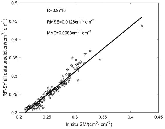
Figure 13.
Linear regression analysis between retrieved SM from RF-SY strategy and in situ SM.
Table 6.
Inversion result accuracy index statistics table.
Although it is feasible and effective to retrieve SM from multi-GNSS and multi-frequency data using the RF model with vegetation effects eliminated through NMRI, the GNSS-IR SM inversion process is also affected by terrain conditions, e.g., surface roughness and vegetation types, and the physical mechanism of the interaction between the reflected signal and the vegetation is still unclear. Moreover, the SM inversion model established for the NJBM station experiment cannot be guaranteed to be applicable to other environments or other stations. All these deserve further investigation.
6. Conclusions
As an important indicator to measure the global water cycle, the long-term accurate monitoring of SM is of great significance and has important application prospects. Based on the limitations of GNSS-IR SM research in the fields of data utilization and application scenarios, an RF SM inversion model based on multi-GNSS and multi-frequency data fusion is proposed with the influence of vegetation effects considered. This study combines vegetation error correction and multi-GNSS and multi-frequency data integration using GNSS-IR multipath data and SNR data. The experimental analysis draws the following conclusions:
- (1)
- The NMRI calculated from MP1 has a strong linear correlation with NDVI, which can fully correct the amplitude and phase offset of the reflected signal caused by the vegetation effects. Therefore, the NMRI calculated by GNSS multipath observations can be used to correct the vegetation error without measuring the VMC.
- (2)
- The RF algorithm gives full play to the advantages of multi-GNSS and multi-frequency data integration in SM inversion and effectively solves the problem that single-satellite data cannot fully reflect the actual situation of the surface. In addition, the addition of threshold and parameter adjustment in the RF model operation process helps to eliminate satellite data that seriously interfere with SM inversion and can determine the satellite combination with a good SM inversion accuracy while ensuring data utilization.
- (3)
- Compared to the traditional MLR and MARS models, the RF model can obtain higher accuracy in the inversion of SM, which can obtain better satellite combinations by adjusting the threshold and parameters. Compared to the proposed RF-AF method, the proposed RF-SY strategy not only has higher accuracy but also reduces the steps of the RF-AF strategy to establish empirical models for each satellite to correct vegetation errors, thereby reducing gross errors and calculation time and increasing the accuracy and efficiency of GNSS-IR SM inversion.
- (4)
- Compared to the single feature parameter (amplitude or phase) fusion correction inversion method, the multi-feature parameter fusion correction inversion method that combines feature parameters extracted from GNSS signals with RF can improve the accuracy and reliability of SM inversion, which provides a new idea for GNSS-IR SM inversion.
In the future, we will continue to observe the NJBM site for a long time to obtain more information about other related vegetation, such as shrubs and trees, to confirm the potential and universality of the technology. At the same time, future research will focus on the physical mechanism of the interaction between vegetation and reflected signals and study the effects of environmental factors, such as soil roughness and soil texture, on SM inversion. Finally, the established SM inversion model will be verified by PBO observation data.
Author Contributions
H.W. designed the experiments, developed the GNSS-IR SM inversion algorithm, supported the study, and wrote the draft; X.Y. processed the multi-GNSS and multi-frequency data and wrote the initial draft; Y.P. established the GNSS site; F.S. supervised the study. All authors have read and agreed to the published version of the manuscript.
Funding
This work was financially supported by Jiangsu Agriculture Science and Technology Innovation Fund (No. CX (21) 3068), and funded by the National Natural Science Foundation of China (No. 42077003).
Data Availability Statement
Data are contained within the article.
Acknowledgments
The authors sincerely thank for the comments from anonymous reviewers and members of the editorial team.
Conflicts of Interest
The authors declare no conflict of interest.
References
- Koster, R.D.; Dirmeyer, P.A.; Guo, Z.; Bonan, G.; Chan, E.; Cox, P.; Gordon, C.T.; Kanae, S.; Kowalczyk, E.; Lawrence, D. Regions of strong coupling between soil moisture and precipitation. Science 2004, 305, 1138–1140. [Google Scholar] [CrossRef] [PubMed]
- Jackson, T.J.; Schmugge, J.; Engman, E.T. Remote sensing applications to hydrology: Soil moisture. Hydrol. Sci. J. 1996, 41, 517–530. [Google Scholar] [CrossRef]
- Larson, K.M.; Small, E.E.; Gutmann, E.D.; Bilich, A.L.; Braun, J.J.; Zavorotny, V.U. Use of GPS receivers as a soil moisture network for water cycle studies. Geophys. Res. Lett. 2008, 35. [Google Scholar] [CrossRef]
- Larson, K.M.; Gutmann, E.D.; Zavorotny, V.U.; Braun, J.J.; Williams, M.W.; Nievinski, F.G. Can we measure snow depth with GPS receivers? Geophys. Res. Lett. 2009, 36. [Google Scholar] [CrossRef]
- Larson, K.M.; Ray, R.D.; Nievinski, F.G.; Freymueller, J.T. The accidental tide gauge: A GPS reflection case study from Kachemak Bay, Alaska. IEEE Geosci. Remote Sens. Lett. 2013, 10, 1200–1204. [Google Scholar] [CrossRef]
- Larson, K.M.; Löfgren, J.S.; Haas, R. Coastal sea level measurements using a single geodetic GPS receiver. Adv. Space Res. 2013, 51, 1301–1310. [Google Scholar] [CrossRef]
- Duan, J.J.; Schmude, J.M.; Larson, K.M. Effects of low temperature exposure on diapause, development, and reproductive fitness of the emerald ash borer (Coleoptera: Buprestidae): Implications for voltinism and laboratory rearing. J. Econ. Entomol. 2021, 114, 201–208. [Google Scholar] [CrossRef]
- Zavorotny, V.U.; Larson, K.M.; Braun, J.J.; Small, E.E.; Gutmann, E.D.; Bilich, A.L. A physical model for GPS multipath caused by land reflections: Toward bare soil moisture retrievals. IEEE J. Sel. Top. Appl. Earth Obs. Remote Sens. 2009, 3, 100–110. [Google Scholar] [CrossRef]
- Chew, C.C.; Small, E.E.; Larson, K.M.; Zavorotny, V.U. Effects of near-surface soil moisture on GPS SNR data: Development of a retrieval algorithm for soil moisture. IEEE Trans. Geosci. Remote Sens. 2013, 52, 537–543. [Google Scholar] [CrossRef]
- Larson, K.M.; Small, E.E. Normalized microwave reflection index: A vegetation measurement derived from GPS networks. IEEE J. Sel. Top. Appl. Earth Obs. Remote Sens. 2014, 7, 1501–1511. [Google Scholar] [CrossRef]
- Roussel, N.; Darrozes, J.; Ha, C.; Boniface, K.; Frappart, F.; Ramillien, G.; Gavart, M.; Van de Vyvere, L.; Desenfans, O.; Baup, F. Multi-scale volumetric soil moisture detection from GNSS SNR data: Ground-based and airborne applications. In Proceedings of the 2016 IEEE Metrology for Aerospace (MetroAeroSpace), Florence, Italy, 21–23 June 2016; pp. 573–578. [Google Scholar]
- Larson, K.M.; Small, E.E.; Gutmann, E.; Bilich, A.; Axelrad, P.; Braun, J. Using GPS multipath to measure soil moisture fluctuations: Initial results. GPS Solut. 2008, 12, 173–177. [Google Scholar] [CrossRef]
- Larson, K.M.; Braun, J.J.; Small, E.E.; Zavorotny, V.U.; Gutmann, E.D.; Bilich, A.L. GPS multipath and its relation to near-surface soil moisture content. IEEE J. Sel. Top. Appl. Earth Obs. Remote Sens. 2009, 3, 91–99. [Google Scholar] [CrossRef]
- Lv, J.; Zhang, R.; Tu, J.; Liao, M.; Pang, J.; Yu, B.; Li, K.; Xiang, W.; Fu, Y.; Liu, G. A GNSS-IR Method for Retrieving Soil Moisture Content from Integrated Multi-Satellite Data That Accounts for the Impact of Vegetation Moisture Content. Remote Sens. 2021, 13, 2442. [Google Scholar] [CrossRef]
- Zhan, J.; Zhang, R.; Xie, L.; Li, S.; Lv, J.; Tu, J. Vegetation Growth Monitoring Based on BDS Interferometry Reflectometry with Triple-Frequency SNR Data. IEEE Geosci. Remote Sens. Lett. 2022, 19, 1–5. [Google Scholar] [CrossRef]
- Chew, C.C.; Small, E.E.; Larson, K.M.; Zavorotny, V.U. Vegetation sensing using GPS-interferometric reflectometry: Theoretical effects of canopy parameters on signal-to-noise ratio data. IEEE Trans. Geosci. Remote Sens. 2014, 53, 2755–2764. [Google Scholar] [CrossRef]
- Chew, C.; Small, E.E.; Larson, K.M. An algorithm for soil moisture estimation using GPS-interferometric reflectometry for bare and vegetated soil. GPS Solut. 2016, 20, 525–537. [Google Scholar] [CrossRef]
- Small, E.E.; Larson, K.M.; Braun, J.J. Sensing vegetation growth with reflected GPS signals. Geophys. Res. Lett. 2010, 37. [Google Scholar] [CrossRef]
- Small, E.E.; Larson, K.M.; Smith, W.K. Normalized microwave reflection index: Validation of vegetation water content estimates from Montana grasslands. IEEE J. Sel. Top. Appl. Earth Obs. Remote Sens. 2014, 7, 1512–1521. [Google Scholar] [CrossRef]
- Li, S.; Jing, H.; Yuan, Q.; Yue, L.; Li, T. Investigating the spatio-temporal variation of vegetation water content in the western United States by blending GNSS-IR, AMSR-E, and AMSR2 observables using machine learning methods. Sci. Remote Sens. 2022, 6, 100061. [Google Scholar] [CrossRef]
- Pan, Y.; Ren, C.; Liang, Y.; Zhang, Z.; Shi, Y. Inversion of surface vegetation water content based on GNSS-IR and MODIS data fusion. Satell. Navig. 2020, 1, 1–15. [Google Scholar] [CrossRef]
- Zhang, S.; Wang, T.; Wang, L.; Zhang, J.; Peng, J.; Liu, Q. Evaluation of GNSS-IR for retrieving soil moisture and vegetation growth characteristics in wheat farmland. J. Surv. Eng. 2021, 147, 4021009. [Google Scholar] [CrossRef]
- Liang, Y.; Ren, C.; Wang, H.; Huang, Y.; Zheng, Z. Research on soil moisture inversion method based on GA-BP neural network model. Int. J. Remote Sens. 2019, 40, 2087–2103. [Google Scholar] [CrossRef]
- Larson, K.M.; Small, E.E. GPS ground networks for water cycle sensing. In Proceedings of the 2014 IEEE Geoscience and Remote Sensing Symposium, Quebec City, QC, Canada, 13–18 July 2014; pp. 3822–3825. [Google Scholar]
- Larson, K.M. GPS interferometric reflectometry: Applications to surface soil moisture, snow depth, and vegetation water content in the western United States. Wiley Interdiscip. Rev. Water 2016, 3, 775–787. [Google Scholar] [CrossRef]
- Small, E.E.; Larson, K.M.; Chew, C.C.; Dong, J.; Ochsner, T.E. Validation of GPS-IR soil moisture retrievals: Comparison of different algorithms to remove vegetation effects. IEEE J. Sel. Top. Appl. Earth Obs. Remote Sens. 2016, 9, 4759–4770. [Google Scholar] [CrossRef]
- Yuan, Q.; Li, S.; Yue, L.; Li, T.; Shen, H.; Zhang, L. Monitoring the Variation of Vegetation Water Content with Machine Learning Methods: Point–Surface Fusion of MODIS Products and GNSS-IR Observations. Remote Sens. 2019, 11, 1440. [Google Scholar] [CrossRef]
- Zheng, N.; Chai, H.; Chen, L.; Ma, Y.; Tian, X. Snow depth retrieval by using robust estimation algorithm to perform multi-SNR and multi-system fusion in GNSS-IR. Adv. Space Res. 2023, 71, 1525–1542. [Google Scholar] [CrossRef]
- Liang, Y.; Lai, J.; Ren, C.; Lu, X.; Zhang, Y.; Ding, Q.; Hu, X. GNSS-IR multisatellite combination for soil moisture retrieval based on wavelet analysis considering detection and repair of abnormal phases. Measurement 2022, 203, 111881. [Google Scholar] [CrossRef]
- Ding, R.; Zheng, N.; Zhang, H.; Zhang, H.; Lang, F.; Ban, W. A Study of GNSS-IR Soil Moisture Inversion Algorithms Integrating Robust Estimation with Machine Learning. Sustainability 2023, 15, 6919. [Google Scholar] [CrossRef]
- Wang, X.; Zhang, Q.; Zhang, S. Water levels measured with SNR using wavelet decomposition and Lomb–Scargle periodogram. GPS Solut. 2017, 22, 22. [Google Scholar] [CrossRef]
- Wang, X.; Zhang, Q.; Zhang, S. Sea level estimation from SNR data of geodetic receivers using wavelet analysis. GPS Solut. 2018, 23, 6. [Google Scholar] [CrossRef]
- Wang, X.; He, X.; Xiao, R.; Song, M.; Jia, D. Millimeter to centimeter scale precision water-level monitoring using GNSS reflectometry: Application to the South-to-North Water Diversion Project, China. Remote Sens. Environ. 2021, 265, 112645. [Google Scholar] [CrossRef]
- Zhou, W.; Liu, Y.; Huang, L.; Ji, B.; Liu, L.; Bian, S. Multi-constellation GNSS interferometric reflectometry for the correction of long-term snow height retrieval on sloping topography. GPS Solut. 2022, 26, 140. [Google Scholar] [CrossRef]
- Camps, A.; Alonso-Arroyo, A.; Park, H.; Onrubia, R.; Pascual, D.; Querol, J. L-band vegetation optical depth estimation using transmitted GNSS signals: Application to GNSS-reflectometry and positioning. Remote Sens. 2020, 12, 2352. [Google Scholar] [CrossRef]
- Evans, S.G.; Small, E.E.; Larson, K.M. Comparison of vegetation phenology in the western USA determined from reflected GPS microwave signals and NDVI. Int. J. Remote Sens. 2014, 35, 2996–3017. [Google Scholar] [CrossRef]


Disclaimer/Publisher’s Note: The statements, opinions and data contained in all publications are solely those of the individual author(s) and contributor(s) and not of MDPI and/or the editor(s). MDPI and/or the editor(s) disclaim responsibility for any injury to people or property resulting from any ideas, methods, instructions or products referred to in the content. |
© 2023 by the authors. Licensee MDPI, Basel, Switzerland. This article is an open access article distributed under the terms and conditions of the Creative Commons Attribution (CC BY) license (https://creativecommons.org/licenses/by/4.0/).