The millimeter-wave radar array was compared with a capacitive wave height meter in a wave tank and compared with RADAC’s WG5-HT-CP radar in offshore marine conditions. The validation of the millimeter-wave radars is described as follows.
4.2.1. Experiments in Planar Random-Wave Wave–Current Coupling Pool
The capacitive wave height meter developed by Tianjin Water Transport Engineering Survey and Design Institute, located in Tianjin, China, was used to collect and monitor the wave surface elevation of the planar random-wave wave–current coupling pool in real time. As shown in
Figure 5a, the capacitive wave height meter adopts a two-wire structure, which has the characteristics of high measurement accuracy and small linear error compared with the single-wire capacitive wave height meter. Its working principle is that the inter-line capacitance of the capacitive sensing wire changes in real time as the water level changes. The capacitance value can be converted into the wave height, that is, the water depth, via the signal acquisition chip. The effective range of the capacitive wave height meter is 60 cm.
Figure 5b is a 32-channel experimental data collector supporting the capacitive wave height meter.
The capacitive wave height meter was installed in the planar random-wave wave–current coupling pool, and it measured the wave height of the tank at a frequency of 100 Hz. The data were collected using a high-speed data acquisition system with 64 channels. The millimeter-wave radar array was installed on the bridge above the wave tank, vertically illuminating the water surface and providing the vertical distance between the radar and the water surface at a sampling frequency of 20 Hz. The measurements between the capacitive wave height meter and the millimeter-wave radars were not affected by each other. Two sets of regular wave measurement data were named Re013 and Re014, while three sets of irregular wave data were named Irre003, Irre004, and Irre006. The millimeter-wave radars and the capacitive wave height meter simultaneously collected data. The data collection times for Re013, Re014, Irre003, Irre004, and Irre006 were 250.1 s, 250.1 s, 350.05 s, 350.05 s, and 315.05 s, respectively.
Figure 6a,b is a comparison of two sets of wave height time series samples collected with the millimeter-wave radars and the capacitive wave height meter. Since the millimeter-wave radars and the capacitive wave height meter were in different locations in the pool, the time was aligned. It can be seen in
Figure 6a,b that the wave height time series measured with the millimeter-wave radars agreed well with those measured with the capacitive wave height meter, and the error is reflected in Table 5.
Figure 7a is inverted from the data set Re013, and
Figure 7b is inverted from the data set Irre006. In
Figure 7a, it can be observed that under regular wave conditions, there was good agreement between the frequency spectra measured with the millimeter-wave radars and the capacitive wave height meter, enabling the effective resolution of various frequency components. Compared with the capacitive wave height meter, the wave spectrum measured with the millimeter-wave radars exhibited a narrower spectral width and lower spectral peak at most wave frequency components. In the case of irregular waves, the main peak frequency and amplitude of the two were in good agreement, as shown in
Figure 7a,b. The millimeter-wave radar emits a beam that illuminates an area footprint, while the capacitive wave height meter measures the wave height at a specific point. Therefore, the raw wave height data collected with the millimeter-wave radars exhibit an overall high noise level. Median absolute deviation (MAD) outlier detection, smoothing, and singular spectrum analysis (SSA) were performed on the millimeter-wave radar wave height data, effectively reducing the noise level in the radar-measured spectrum at high frequencies. Although the spectral noise at high frequencies was reduced after the denoising and smoothing processing of the measured data with the millimeter-wave radars, the spectral amplitude at the main frequency components also decreased.
The designed wave parameters for the planar random-wave wave–current coupling pool are presented in
Table 3. As the wave parameters in the wave tank were expected values, the actual wave parameters were considered to be the values measured with the capacitive wave height meter.
Table 4 and
Table 5 present the wave parameters obtained with the capacitive wave height meter and the millimeter-wave radars. In the case of regular waves, the millimeter-wave radars exhibited an average deviation of 0.025 m for a significant wave height and 0 s for the dominant wave period compared with the capacitive wave height meter. In the case of irregular waves, the millimeter-wave radars showed an average deviation of 0.008 m for a significant wave height and 0.017 s for the dominant wave period.
A millimeter-wave radar array composed of multiple millimeter-wave radars was deployed in the planar random-wave wave–current coupling pool.
Figure 8a,b,
Figure 9a,b and
Figure 10a,b illustrate the arrangement of the millimeter-wave radar array and the direction of the water waves in the cases of regular and irregular waves, respectively. In
Figure 8a,
Figure 9a and
Figure 10a, the x-axis points toward one end of the wave-absorbing pool.
Figure 8b shows one end of the wave-making end. In
Figure 8b, the wave direction is from one end of the wave-making end to the wave-absorbing end, and the wave peak is parallel to the edge of the wave-making pool.
Figure 9b represents the wave-absorbing end. The wave propagation direction in
Figure 9b is from the wave-making end to the wave-absorbing end, and the wave peak is parallel to the wave-absorbing end.
Figure 10a,b and
Figure 11a,b depict the wave direction spectrum obtained with the millimeter-wave radar array under regular and irregular wave conditions, respectively. The wave height time series collection time used for the inverted wave direction spectrum in
Figure 10 was 190.1 s, and the wave height time series collection time used for the inverted results in
Figure 11 was 301 s. In the two-dimensional wave directional spectra, 270° represents one end of the wave generator in the planar random-wave wave–current coupling pool, and 90° represents the other end of the pool. The directions in the two-dimensional wave directional spectra represent the directions in which waves go.
In
Figure 10b, the energy-dense region of the wave direction spectrum for regular waves has a narrow frequency range, and the peak frequency amplitude is 2–6 orders of magnitude higher than the other frequency components. Therefore, in
Figure 10b, only the peak frequency is visible. Furthermore, the energy around 270° in
Figure 10b is considered to be waves reflected from one end of the wave pool. In
Figure 8b, the wave propagation direction is depicted, with the direction being toward one end where the wave absorber is located. By comparing with the actual direction, it can be observed that the wave direction observed with the millimeter-wave radar arrays aligned with reality, with the center of the energy-dense region at approximately 96°. The measured wave direction was not precisely 90°, which could be attributed to slight deviations between the actual wave generation direction in the planar random-wave wave–current coupling pool and 90°, or it may be related to the positioning offset of the millimeter-wave radar array.
Figure 11a,b depicts the wave direction spectra measured with a T-shaped array of four millimeter-wave radars. Compared with regular waves, the spectrum peaks of the measured wave direction spectrum for irregular waves are broader and flatter rather than having sharp individual peaks, as observed in the wave direction spectrum for regular waves. Therefore, in
Figure 11a,b, the wave direction spectra exhibit larger spectral widths. The direction at which the energy peak of the wave direction spectrum occurs is approximately 80°.
4.2.2. Field Experiment in the Ocean
The millimeter-wave radar was installed on a tripod attached to the bridge railing, with the support frame’s horizontal plane parallel to the sea surface. The WG5-HT-CP wave-measuring radar produced by RADAC was mounted on a stable bracket at the bridge railing, emitting electromagnetic waves that incident vertically on the sea surface. The on-site arrangement of the instruments is shown in
Figure 12. The millimeter-wave radar measured the instantaneous height between the radar and the sea surface and was equipped with a custom data acquisition system. When the millimeter-wave radar was powered on, the data acquisition system recorded wave height values 20 times per second. The WG5-HT-CP wave measurement radar measured the distance to the water surface 10 times per second, and the data were stored internally and distributed through the network. Any device connected to the (dedicated) network could access the web-based user interface. A comparative analysis of the measurement results from both systems will be conducted.
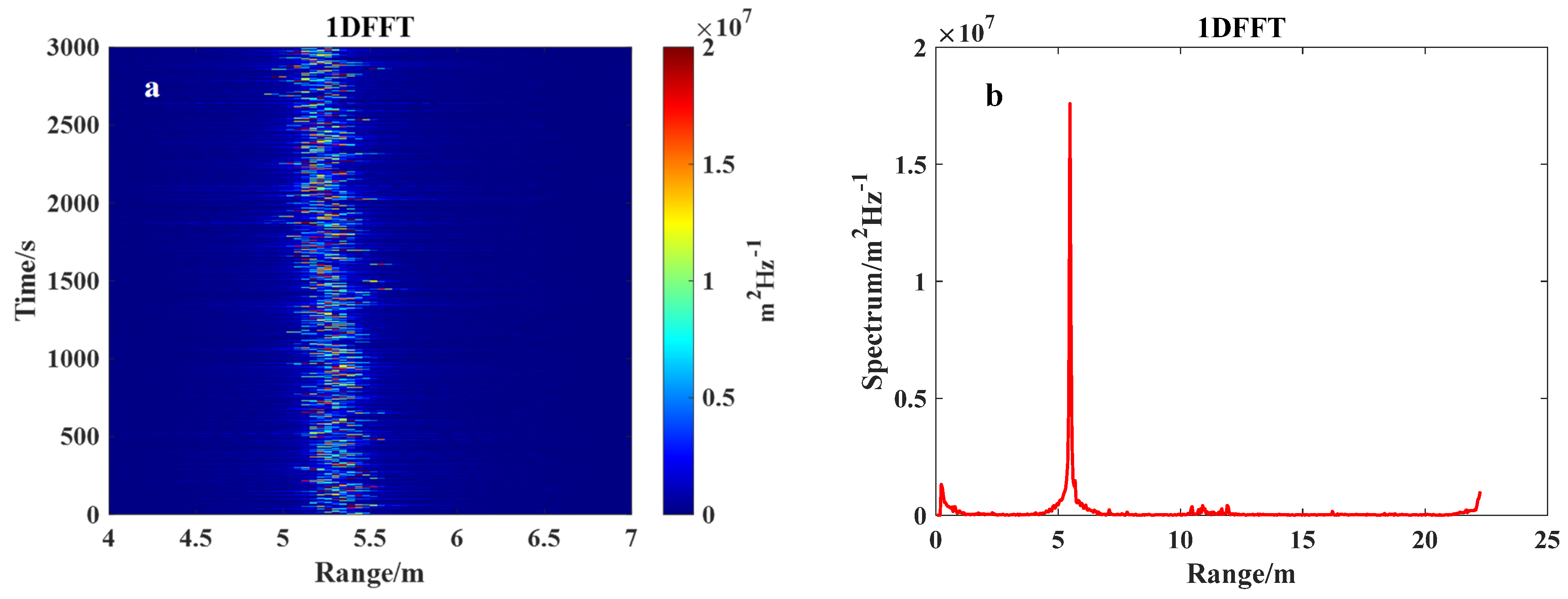
Figure 13 presents the comparative results of the frequency spectra measured with the millimeter-wave radar and the WG5-HT-CP radar. The millimeter-wave radar and WG5-HT-CP radar simultaneously collected data, with a data collection time of 1199 s. The comparative analysis of the frequency spectra revealed a relative consistency in the main peak frequencies between the millimeter-wave radar and the WG5-HT-CP radar, with comparable magnitudes of the spectra.
Figure 14 presents the scatter plots of significant wave height, spectrum peak period, mean wave period, and mean zero-crossing wave period measured with the millimeter-wave radar and the WG5-HT-CP radar over the observation period. The millimeter-wave radar and WG5-HT-CP radar simultaneously collected data, with a data collection time of 3240 s. Each point in the scatter plot was calculated at 2-min intervals. The three wave period parameters are distributed near the diagonal line, but the distribution of significant wave height tends toward the lower right corner. The significant wave heights measured with the millimeter-wave radar are generally 2–3 cm higher than those measured with the WG5-HT-CP radar, possibly due to radar calibration errors.
Table 6 presents the standard deviation, root mean square error, and mean bias of the significant wave height, spectrum peak period, mean wave period, and mean zero-crossing wave period measured with the millimeter-wave radar compared with the WG5-HT-CP radar. The standard deviation, root mean square error, and mean bias of the significant wave height are 0.019 m, 0.026 m, and 0.022 m, respectively, all in the centimeter range. The standard deviation, root mean square error, and mean bias of the wave periods are within the range of 0.210–0.329 s, showing close agreement with the wave periods measured with WG5-HT-CP.
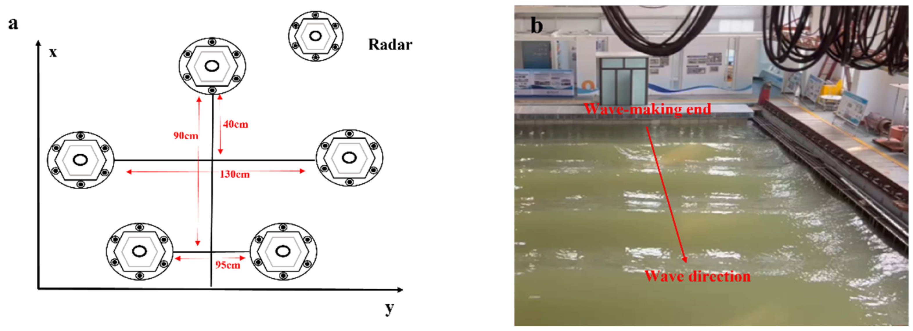
An array consisting of at least three instruments can be used to measure the wave direction. A millimeter-wave radar array was deployed on a fixed T-shaped rigid structure on the bridge deck, with the array distributed in an isosceles triangle configuration, as shown in
Figure 15. According to spatial sampling theory, radars spaced 3 m apart cannot accurately capture waves with wavelengths below 3 m. Therefore, in order to correctly measure high-frequency waves, the array size should not be too large. The plane of the millimeter-wave radar array was positioned parallel to the sea surface, and its emitted electromagnetic waves incident vertically onto the sea surface, resulting in the strongest reflection intensity. The millimeter-wave radar array recorded the vertical distance to the sea surface, and the wave spectrum was obtained using the periodogram method, while the wave direction spectrum was obtained using the BDM method. The measured wave direction spectrum was compared with the actual conditions.
Figure 16a shows the distribution of the millimeter-wave radar array, and
Figure 16b shows the actual propagation direction of the waves in the field. The direction was defined such that northward corresponded to 0°, and waves propagating eastward corresponded to 90°.
Figure 16c represents the wave direction spectrum of the millimeter-wave radar array measurements, while
Figure 16d displays the polar coordinate form of the measured wave direction spectrum. It can be observed that the direction distribution was primarily in the northeast direction, with the peak energy located at approximately 15° east of north, consistent with the actual wave direction. The measured marine area is located in the nearshore region, where in addition to waves propagating from the ocean toward the coast, waves are reflected from the coastline into the sea. The irregularities in the nearshore seabed topography and coastline can influence the propagation direction of the waves, resulting in variations and uncertainties in wave direction. In addition, the interaction between waves in the nearshore region can lead to phenomena such as wave reflection and interference, further increasing the complexity of the wave direction.


