1. Introduction
Lightning discharges are transients of high current that occur in the Earth’s atmosphere and produce Lightning Electromagnetic Pulses (LEMPs). These signals can be remotely recorded by electric field measurement systems and can be employed in lightning geolocation, modeling, and warning systems, among other applications.
In general, there are two types of lightning: cloud-to-ground (CG), which reaches the ground, and intracloud (IC), which does not involve the ground. The ICs represent about three-quarters of lightning discharges that occur on Earth [
1]. LEMPs generated by lightning processes inside the cloud are different from those generated when lightning strikes the ground. The electrical discharge generated when lightning strikes the ground is called return-stroke, and typical LEMP return-stroke waveforms measured at a distance beyond several tens of kilometers or so are characterized by a short rise time and a relatively slow decay time [
2,
3,
4,
5]. On the other hand, LEMP waveshapes produced by intracloud lightning processes are very diverse, and it is difficult to draw a typical waveform for IC LEMPs. However, they are generally narrower than LEMPs produced by return strokes. For long distances between the CG lightning channel and the measuring station (beyond 100 km or so), it is possible to observe a subsequent peak after the main one. Those peaks are related to the so-called “skywaves”. The skywaves are electromagnetic signals propagating from the lightning channel, reflecting on the waveguide formed by the ionosphere and ground, and reaching the sensor.
The stochastic characteristics of lightning in time and space make it difficult to study. Methodologies that classify events and define what types of lightning are occurring are very important in the analysis of thunderstorm dynamics in each region, favoring the decision making of adequate security measures to avoid deaths and financial losses.
Williams et al. [
6] studied the correlation between severe weather and total lightning flash rates. They showed evidence that severe weather manifestations on the ground are preceded by a rapid increase in the intracloud flash rate. Chkeir et al. [
7] used the number of lightning strikes, their height of occurrence, and their type to nowcast extreme rain and extreme windspeed (severe weather). According to the authors of [
8,
9], Narrow Bipolar Events (NBEs) or Compact Intracloud Discharges (CIDs) can be indicators of severe convection in thunderstorms. Measurements carried out by the Los Alamos Sferic Array (LASA) showed an increase in the heights of NBEs during the intensification of convective elements in the eyewall of hurricanes Rita and Katrina in 2005 [
10].
Some studies have shown that changes in the concentration of aerosols in the atmosphere influence lightning activity. Liu et al. [
11] showed that the increase in aerosol invigorates positive IC strokes and negative CG strokes in thunderstorms. In [
12,
13], the authors related the anthropogenic increase in aerosol concentration in large urban centers to the decrease in positive CG. From a different point of view, smoke aerosol caused by forest fires contributes to the increase in positive lightning [
14,
15,
16]. The final stage of Tropical Cyclones (TCs) is usually accompanied by intense positive CG lightning activity. This behavior was reported during hurricanes Emily, Rita, and Katrina in 2005 [
17].
From the above, the lightning type is correlated to a variety of atmosphere/thunderstorm conditions. Hence, knowing the correct type of lightning flash is of interest to different research subjects, from aerosol pollution to severe weather.
One of the most common ways to obtain LEMPs is by using lightning electric field measuring systems [
18]. A way to differentiate IC from CG events is by using the waveform’s rise and fall time and its signal-to-noise ratio [
19]. However, due to the variety of processes that occur in a flash, this statistical method is recommended for a single pulse flash or the study of a specific thunderstorm, since its accuracy in IC lightning is less than 85%, and in CG, it is between 70 and 80% [
20].
Most of the regional and continental terrestrial networks (e.g., the U.S. National Lightning Detection Network (NLDN), Earth Networks Total Lightning Network (ENTLN), and European Cooperation for Lightning Detection (EUCLID) network) use multiparameter lightning classification algorithms to differentiate between CG and IC lightning [
21]. The overall classification accuracy for CG lightning varies between 70 and 92% [
22,
23,
24,
25]. Some studies evaluated the accuracy of ICs in specific networks, finding 90% accuracy [
26] and 92% accuracy [
24], both for NLDN, and 73–92% for EUCLID considering only the peak-to-zero (PTZ) time and 91–96% considering the multiparameter lightning classification algorithm [
22].
There are some disadvantages to using multiparameter algorithms for lightning classification. In the work of Biagi et al. [
27], a large number of positive ICs were incorrectly classified as positive CG lightning by the NLDN network. As an attempt to solve this problem, a new criterion was implemented, in which the estimated peak current amplitude is used to differentiate positive pulses between positive CG and positive IC, although this implies a misclassification of low-intensity positive CG pulses [
28].
Another classification issue concerns differentiating between CIDs and positive CG. According to Leal et al. [
29], 78% of 1022 CIDs were incorrectly classified as positive CG by the NLDN, and 56% by the ENTLN, and most of the misclassifications were related to high-intensity CIDs.
Another approach to performing lightning classification instead of multiparameter algorithms is applying so-called Artificial Intelligence (AI). AI is a combination of different Machine Learning Algorithms (MLAs) including deep learning and others. These algorithms can learn complex patterns and behaviors from a representative training dataset in order to perform a specific task. Further, we discuss a few approaches found in the literature on lightning classification using AI.
To the best of our knowledge, Eads et al. [
30] were the first to introduce the use of ML in the lightning-type classification task. Their methodology employed genetic algorithms for feature extraction and Support Vector Machines (SVMs) for classification. The dataset used was composed of FORTE Very High Frequency (VHF) satellite data, with 800-microsecond time windows at a 50 MHz sampling rate. The SVM model was responsible for classifying the data into seven different classes: Positive Initial Return Stroke, Negative Initial Return Stroke, Subsequent Negative Return Stroke, Impulsive Event, Impulsive Event Pair, Gradual Intra-Cloud Stroke, and Off-record. Using 10-fold cross-validation, the algorithm named Zeus achieved 61.54% accuracy. The authors also noted that the SVM alone, without the use of feature extraction, achieves 70.38% accuracy.
Wang et al. [
20] developed a 10-type lightning classifier based on a One-Dimensional Convolutional Neural Network (1D-CNN). Their dataset was composed of 50,000 lightning electric field waveforms (slipped equally into 10 different classes) recorded in the VLF/LF (3 kHz–400 kHz) band. The sample rate was 1 MSPS (Million Samples per Second), with a pre-trigger of 100 µs and a post-trigger of 900 µs. Zero-phase digital filtering was used to reduce high-frequency noise. Then, the data were normalized by the z-score normalization technique, in the range from 0 to 1. Each event consisted of 1000 data points. The five-fold cross-validation method was used to find the generalized performance of the model. The accuracy was used as the evaluation metric. The average accuracy for the 10 types of lightning studied was 99.11%, with the lowest being 97.83% and the highest being 99.95%. The algorithm was also used in another 9647 events, which occurred in Hunan, China, on 6 June 2019. The average classification accuracy obtained was 97.55%.
Zhu et al. [
21] implemented a SVM classifier to differentiate lightning between +CG, +IC, −CG, and −IC. They used data from the Cordoba Marx Meter Array (CAMMA) as the ground truth, classifying the lightning pulses by their reported height. Lightning sources whose CAMMA-reported altitudes were less than 1.2 km were classified as CG lightning. If the reported height was greater than 3.2 km, the event was classified as IC. For all these labeled data, a manual confirmation was carried out to ensure that the waveforms had CG or IC characteristics. Within the range between 1.2 km and 3.2 km, data have been removed due to uncertainty in the lightning type classification. Their dataset was composed of 31,005 events, distributed across 543 +CGs, 912 −CGs, 18,249 +ICs, and 11,301 −ICs. The electric field waveforms were 100 µs long (±50 µs with t = 0 at pulse peak). They applied training/testing data of an 80/20 split ratio and four-fold cross-validation to find the best hyperparameters of the model. As the number of IC events was much larger than the number of CG events, the authors oversampled the CG pulses in the training stage to reduce data imbalance caused by the duplication of CG data. The overall accuracies for the training and testing dataset were 97%.
We noticed that machine learning algorithms have higher performance in comparison to multiparameter algorithms for lightning-type classification. The constant improvements in the ML field show us that soon, most of the Lightning Location Systems (LLS) will incorporate those types of algorithms to improve their performance in lightning-type classification.
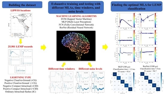
In this study, we assess the performance of different MLAs, including a SVM (Support Vector Machine), MLP (Multi-Layer Perceptron), FCN (Fully Convolutional Network), and Residual Neural Network (ResNet) in the task of LEMP classification. The choice of the MLAs was based on previous attempts at lightning classification [
20,
21] and MLAs that work better with time series [
31]. We also address different aspects of the dataset that can interfere with the problem of lightning-type classification. We assess the length of the recorded LEMP, noise level, and the imbalance in the datasets. To test the different ML algorithms and methodologies, we use a dataset composed of 25,901 LEMPs recorded by the Lightning Detection and Waveform Storage System (LDWSS) in three different locations of the American continent, including the South and North hemispheres.
2. Data and Methodology
The LEMPs used in this work were acquired by the LDWSS operating in wideband (160 Hz–500 kHz). The polarity of lightning electric field waveforms recorded by the LDWSS is based on the atmospheric electricity sign convention, according to which a downward-directed electric field (or electric field change) vector is assumed to be positive. The LDWSS consists of a whip antenna followed by an integrator and a unity-gain, low-noise amplifier. The signal from the pre-amplifier is digitized at 1 MSPS (one million samples per second). The digitizing system has a RTC (Real-Time Clock) which is synchronized with a GPS module. More information about the LDWSS can be found in [
32,
33].
The dataset used in this study is composed of 25,901 LEMPs that occurred in 3 different locations (Gainesville, FL, USA; Belém, PA, Brazil; and Marabá, PA, Brazil).
Figure 1 shows the location of the LDWSS stations and the percentage of LEMPs per location. The LEMPs were recorded during different thunderstorms between 2019 and 2020.
2.1. Preprocessing
All the LEMP waveforms in our dataset have a length (window) of 1.1 ms in which the lightning electric field peak is located at 100 µs. Because of the 1 MHz sampling rate, all the windows (events) have 1100 samples. Further, each event is normalized relative to the peak amplitude at 100 µs to eliminate the effect of amplitude scaling.
We chose five distinguish labels, including Negative Cloud-to-Ground (−CG), Positive Cloud-to-Ground (+CG), Negative Compact Intracloud (−CID) or Low-altitude CIDs, Positive Compact Intracloud (+CID) or High-altitude CIDs, and ordinary Intracloud flashes (IC).
Figure 2 shows the distribution of waveforms in each of the five classes. Examples of typical waveforms of these five classes are shown in
Figure 3.
We did not apply any digital filter in the waveforms of the dataset. However, we measured the average noise level relative to the waveform peak. We consider the noise level as the ratio between the average level of the first 40 µs of each LEMP and the LEMP peak. We found that the average noise level in our dataset is about 2.5%. We also computed the noise level for all classes (see
Figure 4). The class with the highest noise level is IC, with about 4%. The class with less noise is +CID, with about 1%.
2.2. Machine Learning Algorithms (MLAs)
In this paper, four different MLAs were tested and compared to assess the most appropriate approach for LEMP classification. LEMPs can be viewed as a time series because the lightning electric field samples change over time. The choice of the four MLAs is based on previous attempts at lightning classification and MLAs that work better with time series.
In machine learning, a SVM is a supervised learning model used in classification tasks. The SVM is a robust model, having its theoretical basis on the Vapnik–Chervonenkis theory, where a hyperplane or a hyperplane set is created in a high-dimensional or infinite-dimensional space. Intuitively, a satisfying separation is achieved by the hyperplane that features a greater distance to the nearest training point from any class. In general, the greater the margin, the lower the generalization error of the classifier. For classification in problems whose data are not linearly separable, the SVM uses Kernel functions that increase the data space and allow a linear separation [
34]. Our SVM classifier’s C value is set to 1, and its kernel function is the Radial Basis Function (RBF).
The MLP is a kind of Deep Neural Network (DNN) architecture and is often referred to as a feedforward neural network. MLPs are commonly used in a variety of tasks, including classification, regression, and pattern recognition [
35]. MLPs are known for their ability to learn patterns from complex data structures, even when there are non-linear relationships involved, due to their activation functions. However, they may suffer from overfitting when there is not sufficient data to learn from or when the model is too high capacity for the task at hand. Regularization techniques and careful hyperparameter tuning can help mitigate this issue.
The implemented MLP in this work comprises 3 stacked fully connected layers, each containing 500 neurons, ending in a softmax layer. At each layer’s input, dropout rates of 0.1, 0.2, 0.2, and 0.3 are used, and the ReLU activation function is added to increase the non-linearity response.
Figure 5 shows the network structure. The model structure and parameters are shown in
Table 1.
FCNs have been extensively used in semantic segmentation [
36,
37,
38] and image processing [
39] as well as in time series classification tasks [
31].
The implemented FCN comprises a convolutional block that contains a convolutional layer followed by a batch normalization layer and a ReLU activation layer. In total, 3 convolutional blocks are chained together, and the convolutions are performed with kernel sizes of 8, 5, and 3, respectively. The respective filter sizes of the convolutions are 128, 256, and 128. A Batch Normalization layer follows the chained convolutions to speed up and stabilize the convergence of the model. Then, the features are fed up to a Global Average Pooling layer to reduce the number of weights needed in the final Dense layer that gives the probabilities of each label using the softmax activation function.
Figure 6 shows the FCN structure. The model structure and parameters are shown in
Table 2.
ResNets come to solve the degradation problems encountered in deeper networks by adding the shortcut connection, a linear layer from the input to the output of each residual block that allows the model to learn more complex patterns in the data [
31]. Wang et al. [
31] experimented using a ResNet in time series classification tasks and achieved premium performance, even with a deeper structure.
Our ResNet follows the baseline presented in [
31] and is composed of 3 stacked residual blocks that contain 3 convolutional blocks inside, and the input of each residual block is connected via a linear layer to its output. The convolutional blocks of the residual units are the same as in the FCN; the only difference is that the number of filters is 64, 128, and 128, respectively, as shown in
Figure 7. Similar to the FCN, the features are fed up to a Global Average Pooling layer to reduce the number of weights needed in the final Dense layer that gives the probabilities of each label using the softmax activation function. The model structure and parameters are shown in
Table 3.
2.3. Evaluation Metrics
There are several metrics that are commonly used to evaluate the performance of MLAs, namely classification accuracy, precision, recall, and F-score. The classification accuracy expresses the probability of a given sample being correctly classified by the classifier but does not provide information about the number of correct labels of different classes [
40]. Precision denotes the classifier’s ability to minimize false positives (FP) and it is a function of true positives (TP) and FP. Recall, on the other hand, conveys the classifier’s ability to minimize false negatives (FN) and it is a function of TP and FN. The F-score is a composite measure and can be calculated by the harmonic mean between precision and recall. A balance that equally favors precision and recall is achieved when
, resulting in the F1-score.
In this paper, we present all the metrics, but we use the macro-averaged F1-scores to say which model performed better. Macro averaging is essential when dealing with an imbalanced dataset because it treats all classes equally [
41,
42]. The F-score summarizes precision and recall values and is better suited than accuracy to evaluate the classifier’s performance given an imbalanced dataset [
43].
The SVM was evaluated using stratified 5-fold cross-validation, holding 80% of the overall dataset to the training subset and 20% to the test subset. Each evaluation metric is calculated as the average of all 5 test sets. This is performed to reduce variability in the evaluation process and return a more robust performance estimate [
44]. The final models for each different time window are then trained on 80% of the overall dataset and the classification time is measured.
All the other MLAs (MLP, FCN, and ResNet) were trained only once. From the entire dataset, 80% of the samples were drawn to compose the training subset and the remaining 20% were used for testing. A total of 20% of the training subset was used as the validation subset. The training epochs were controlled by the Early Stopping callback in Keras, which monitored the validation loss with a patience value of 50 epochs. The initial learning rate (LR) was set to 0.001 and was systematically reduced by the Reduce Learning Rate On Plateau callback in Keras. The LR reduction occurred when a validation loss plateau was identified by the callback, which decreases the LR by half, with a patience value of 20 epochs. The Model Checkpoint callback in Keras allows us to save the latest best model, monitoring the validation loss. These callbacks help avoid overfitting and help save time in the training process.
Due to lightning distribution in nature and the use of single-station electric-field waveform lightning data, some classes are less represented than others. The +CID class, for example, constitutes less than 1% of the total number of instances, and the +CG class, less than 2%. This can lead to overfitting in the training process and result in non-optimal performance in the minority classes, as the model does not have sufficient examples to learn from. To deal with this issue, we use the Synthetic Minority Oversampling Technique (SMOTE). The SMOTE algorithm systematically introduces new synthetic instances between k minority class nearest neighbors by estimating the difference of one feature vector over its nearest neighbor and randomly scaling this difference, later adding this result to the original feature vector [
45]. All the minority classes (+CG, −CID, +CID, IC) were oversampled to the majority class (−CG) number of instances in the training subset, meaning the test subset was kept unchanged. Because of this, the training subset remains imbalanced, hence we use the F1-score to evaluate the model’s performance.
The Class Activation Map (CAM) helps us to interpret class-specific characteristics in the dataset, indicating the possibly discriminative regions used by the Convolutional-based approaches (FCN and ResNet) to identify certain classes. For a given time series,
represents the activation of the
filter in the last convolutional layer at the point
t in time. The weight of the final softmax function for the
k filter output for each class is represented by
. The CAM is defined by the following equation, where
stands for the CAM for each class
c for each
t point in time:
CAM offers a natural way to explain how convolutional networks work in specific datasets, and with specific configurations. CAM is used in this paper to analyze the best classifier’s performance, and to infer its behaviors.
3. Results
The accuracy, precision, recall, and F1-score metrics are shown for all the approaches. However, we use the macro-averaged F1-score to say which model performed better. Most previous works on the same topic [
20,
21] evaluate the performance of their models mostly using accuracy and, as stated before, it neglects the differences between the types of misclassifications. In other words, the difference in performance between classes are neglected by the accuracy score, hence it is hard to know when a certain class performs poorly. Additionally, looking only at the accuracy may introduce bias in the classifier. The F1-score is a balance between precision and recall and considers TP, FP, TN, and FN, which makes a more robust metric for a multiclass approach.
We assessed the influence of different windows (recorded length) on the classification performance. The window or recorded length of the lightning electric field waveform is a choice of the system designer. The classification algorithm can be implemented with different recorded lengths. For instance, Zhu et al. [
21] used a window of 100 µs, which is a relatively short time window. On the other hand, Wang et al. [
20] used 1000 µs. In both studies, the performance accuracy of the models was higher than 90%. Hence, different time windows can reach satisfactory results. However, if the algorithms are intended to be used in real time, short windows are better. By real time, we mean that the model will classify the LEMPs as they are recorded by the LDWSS. The models can also work in an offline mode, that is, a previously recorded LEMP dataset will be classified at a future time. For instance, we can run the classifier once every day. It is important to note that there is no difference in the algorithm used in “real time” or “offline”.
In order to evaluate the computational effort for each model, we measured the average waveform classification time. The models were executed on a 64-bit Windows 10 laptop (processor: AMD Ryzen 5 5600H at 3.3 GHz) using Tensorflow and Keras in a Jupyter open-source web-based interactive development environment. According to the whole dataset, the average time required for the model to execute the classification algorithm for 25,901 lightning waveforms was measured. The results are shown in
Table 4,
Table 5,
Table 6 and
Table 7. The time shown in
Table 4,
Table 5,
Table 6 and
Table 7 refers only to the classification time, not including the preprocessing time. The fastest model was the MLP across all the different time windows.
We chose four different windows, 1100 µs, 450 µs, 200 µs, and 100 µs, with the peak of the waveform located at 100 µs, 50 µs, 50 µs, and 50 µs, respectively.
Figure 8 shows one example of a LEMP in the four windows.
Figure 9 shows the F1-score versus the classification time for all models, where different colors indicate different time windows. The best performances, characterized by higher values of the F1-score, are related to a long time window (1100 µs). This is highlighted in the green region of
Figure 9. However, for the models trained with the shortest time window (100 µs), the performance of the models can be widely different, varying the F1-score from 37 to 93. This is highlighted in the blue region of
Figure 9. In other words, a good performance does not depend only on the recorded time window, it also depends on which learning model is being used. Therefore, for offline applications, one can use the model that has the best performance regardless of the classification time. However, for real-time applications, a balance must be considered between good performance and how long the algorithm takes to perform the classification.
In
Table 4,
Table 5,
Table 6 and
Table 7, we summarize the results of the metrics. In general, F1-scores are higher when we apply data balance with SMOTE, mainly for shorter windows (450 µs, 200 µs, and 100 µs). For instance, in
Table 4, the F1-score for the FCN model increased from 37.5 to 83.9 when using the SMOTE technique. This same trend was not observed in the MLP model. For MLP, when we use SMOTE the F1-score is lower. In
Table 7, which shows the metrics for the models trained with a 1100 µs time window, the only model that increased its performance (F1-score) due to the use of SMOTE was the SVM. So, the use of data balancing with SMOTE did not bring many benefits in performance for models that use a long time window.
Figure 10a illustrates how the F1-score changes over the different time windows for all models. A performance leap between 450 µs and 1100 µs time windows can be seen in the SVM, FCN, and ResNet classifiers. The leap can be related to how the models deal with the input time-series data. The SVM classifier depends on the separation of the dataset by hyperplane sets and can suffer alteration if we change the arrangement of the input data. FCNs and ResNets are commonly used in deep learning and big data, so it is expected that the more data we feed the model, the better its performance. However, it also depends on the relevance of the input data. If it is not important for learning, this can reduce performance. They both work with convolutional layers, which use filters to extract information from the input data. The difference in the input waveform length can lead to a different characteristic extraction, and then a variability in the performance of the network.
Figure 10b shows how the classification time changes over the different time windows for all models. The classification times for both MLP and MLP_SMOTE are very similar regardless of the time window used. The differences between classification time in MLP models for 200 µs, 450 µs, and 1100 µs time windows are not statistically significant (assuming two times the standard error as a criterion). There is a small difference if we compare the MLP models that use 200 µs, 450 µs, and 1100 µs time windows with the MLP models of a 100 µs window. In general, comparing each individual learning model, with and without the use of SMOTE, they all show similar trend lines. The solid and dashed lines tend to overlap. The only model in which this does not happen is the SVM, which maintains the same tendency, such as increasing the classification time from a 100 µs to a 450 µs window and reducing it from a 450 µs to a 1100 µs window. However, the lines do not overlap.
The SVM, FCN, and ResNet models notably benefit from training with the oversampled dataset, especially when trained with shorter time windows. The MLP model performs at its best when trained with the original training subset. All the models trained with the 1100 µs time window did not benefit from training with the oversampled training subset. SMOTE justifies its use when the time windows are shorter.
In summary, the ResNet trained with no data augmentation (SMOTE) and with a time window of 1100 µs had the best performance overall with an F1-score = 96.67. For the shortest time window (100 µs), the best model was the MLP, with an F1-score = 93.35. In terms of processing time, the MLP (100 µs) is about 6 times faster than ResNet (1100 µs). For a real-time application, the MLP (100 µs) should be considered even though its perforce is 3 percentage points lower than ResNet (1100 µs). In
Figure 11 and
Figure 12, we show the confusion matrix for these two models, MLP (100 µs) and ResNet (1100 µs), respectively. As expected, the confusion matrices show that both models perform the worst in the minority classes (+CG and +CID), where there were fewer data points to train from.
Figure 13 shows the box plot of the Resnet (1100 µs) model’s F1-score. It is interesting to note that in the minority classes (+CG and +CID) there is more variation in performance (F1-score), and in the majority classes (−CG and IC) it is the opposite.
In [
31], the authors encourage the exploration of the ResNet structure in more complex and larger datasets, since it is a very high-capacity model and tends to overfit in smaller and less complex datasets. Our experiments showed that reducing the dataset time window from 1100 µs to 100 µs leads the ResNet to overfit the training data. This behavior is identified by the growing distance between validation and training loss scores, as well as the fluctuation in validation loss values for the 100 µs time window model in contrast to the steady curve for the 1100 µs time window model depicted in
Figure 14a,b.
4. Discussion
To assess how the added noise in the test subset impacts the performance of the models, we introduced three different noise levels (5%, 10%, and 15%) in our LEMPs and tested them against all the models. Examples of LEMPs in the 1100 µs and 100 µs windows with 5%, 10%, and 15% white noise added are shown in
Figure 15 and
Figure 16, respectively. We chose the relative F1-score to compare the models. The relative F1-score is the ratio between the F1-score of models tested with noisy LEMPs and the F1-score of models tested with LEMPs without noise added. A relative F1-score equal to 1 means that the added noise in the test subset did not affect that specific model and a relative F1-score below 1 means that the performance of the model decreased as we introduced the noise.
Figure 17 shows how the relative F1-score changes with the addition of noise in the LEMPs. We also computed what we called the “noise robustness index”, which is the F1-score times the relative F1-score for the models tested with the highest level of noise (15%) added. A high noise robustness index indicates that the model is robust against noisy LEMPs because the high initial F1-score is maintained as we increase the noise level. The noise robustness index for all models (in ascending order) is shown in
Figure 18. The main observations when introducing noise on the test subset are as follows:
Overall, as we increase the noise level, the models tend to perform worse. However, the worst-performing models maintained suboptimal performance (e.g., FCN (100 µs) and the SVM).
In general, models that work with longer time windows performed worse against noise. In other words, we observed bigger drops in performance as we increased the noise level for the models with longer time windows.
The MLP models performed the best against noise. The model with the highest noise robustness index is MLP SMOTE (1100 µs).
For the MLP (100 µs) and ResNet (1100 µs) models, we assess how the classification of different types of LEMPs is affected by the addition of white noise in the test subset (see
Figure 19). We chose these two models for these analyses because MLP (100 µs) was the best model with the fastest performance for the 100 µs window and ResNet (1100 µs) was the overall best model. For both models, +CG and −CID did not decrease their performance much as we increased the noise level. The +CIDs performed worse in both models. Our hypothesis is that the noise easily changes the unique narrow bipolar shape of +CIDs, and then the main features that the MLAs use to classify them are lost. Even though the +CID and −CID waveforms are very similar in the one-dimensional time-series representation, they may manifest different behaviors in the high-dimensional space when fed to the classification models. This can lead to easier or harder separation of these two classes from the other ones, resulting in distinct performances between +CID and −CID when evaluating the noise robustness of these classes. Based on
Figure 19, the MLP (100 µs) shows better capacity at separating and classifying +CID noisy test waveforms than ResNet (1100 µs).
We applied CAM in the ResNet (1100 µs) model to examine what part of the lightning electric field waveform was contributing more to the resulting model.
Figure 3 shows lightning electric field waveforms highlighted with CAM for all the classes used here. We can notice that the model neglects the slow-transition parts of the waveforms. This is depicted by the dark blue parts of the lightning electric field waveforms, which indicates no contribution to the classifier’s decision. The most important parts of the waveforms are the fast transitions located at the peak or near the peak.
Figure 20 shows lightning electric field waveforms for −CG recorded at different distances highlighted with CAM. Note that we do not have distance information, but the distance can be estimated based on the skywaves (peak following the ground wave or first peak [
46,
47]). Even for lightning recorded from far distances in which the lightning electric field waveform has multiple skywaves (multiple peaks), the most important parts of the waveforms are the fast transitions located at the first peak (ground wave). The same trend is seen in +CG, as shown in
Figure 21, and for the intra-cloud events shown in
Figure 22.
This finding is very important because we show for the first time that the MLAs are interested in the ground wave (or direct wave in the case of ICs) of the lightning electric field waveform. Hence, if the waveform is recorded at distances beyond 600 km or so at which the ground wave is degraded, the classification algorithm will not work properly.
5. Summary
In this work, we explore the use of different Artificial Intelligence approaches to classify Lightning Electromagnetic Pulses (LEMPs). We assess the performance (in terms of F1-score) of different MLAs, including the SVM (Support Vector Machine), MLP (Multi-Layer Perceptron), FCN (Fully Convolutional Network), and Residual Neural Network (ResNet) in the task of LEMP classification. To test the different approaches, we use a dataset composed of 25,901 LEMPs recorded by the Lightning Detection and Waveform Storage System (LDWSS) in three different locations on the American continent. We also assessed the influence of different windows (recorded length), noise level, and data balance using the Synthetic Minority Oversampling Technique (SMOTE) on the classification performance. The ResNet trained with no data augmentation (SMOTE), and with a time window of 1100 µs had the best overall performance, with an F1-score = 96.67. In terms of classification speed, as expected, models trained with shorter time windows were faster. Among the fastest models, the one that performed better was the MPL (100 µs), with an F1-score of 92.54. If classification time is a concern, for instance, in real-time applications, MPL (100 µs) is the more appropriate approach to use. Regarding noise level, it was observed that models that work with longer time windows performed worse against noise. Overall, MLP models performed the best against noise. The model with the highest noise robustness index was MLP SMOTE (1100 µs). We applied CAM to the ResNet (1100 µs) model to examine what part of the lightning electric field waveform was contributing more to the resulting model. We noticed that the model neglects the slow transition parts and gives more importance to the fast transitions. We find that the MLAs are interested in the ground wave (or direct wave in the case of ICs) of the lightning electric field waveform. Hence, if the waveform is recorded at distances beyond 600 km or so at which the ground wave is degraded, the classification algorithm will not work properly.


