Evolution of Different Types of Eddies Originating from Different Baroclinic Instability Types

Abstract

This paper investigates the evolution of global eddies and various types of eddies originating from baroclinic instability (BCI) by utilizing satellite altimetry, Argo profiles, and climatology datasets. The structure of global eddies with regard to potential temperature anomalies experiences downward propagation and spreading from the periods of eddy growth to stabilization. However, from the eddy’s stabilization to the decay period, the process of spreading primarily occurs horizontally, and this process is usually accompanied by weakening. By comparing the evolution of eddies in three typical regions dominated by distinct types of BCI, we found that the basic properties of eddies related to different BCI types evolve similarly; however, there are notable differences in their vertical structures and evolution. Eddies associated with Phillips + Charney_s-type, Charney_s-type, and Eady-type BCIs exhibit dual-core, single-core, and dual-core structures, respectively. In particular, the intrusion of the Okhotsk cold water mass into the Northwest Pacific region forms cold-core anticyclonic eddies, resulting in AEs that are significantly distinct from the rest of the ocean. The evolution of surface-layer cores closely resembles that of the global eddies, while the decay of subsurface and bottom-layer cores is comparably sluggish. Additionally, we examine the impact of local oceanic stratification conditions on eddy decay and determine that stronger vertical gradients result in more vigorous eddy decay, accounting for the concentration of eddies at depths where vertical gradients are weaker during their evolution.

1. Introduction

Mesoscale eddies are widely distributed and dominate the ocean’s kinetic energy at mesoscale scales ranging from tens to hundreds of kilometers [1,2,3]. They have a significant impact on oceanic mass, momentum, heat, salt, nutrients, and chlorophyll redistribution [4,5,6,7,8,9,10,11,12]. Mesoscale eddies are the primary destination for the energy generated by large-scale ocean circulation due to equilibrium instabilities. The instability process mainly involves barotropic instability and baroclinic instability (BCI) as outlined by Vallis [13]. Mesoscale eddies also perform a critical function in ocean energy dissipation [14,15], transferring energy from large-scale circulation to submesoscale motions. The final flow of energy is strongly influenced by the evolutionary process of eddies. However, the structure evolution of eddies remains an unresolved issue.

BCI is the primary mechanism for generating eddies, with the majority of eddies thought to be produced through this process [16,17,18,19]. Researchers [20,21,22] conducted linear stability analyses on global ocean density and current velocity, obtaining growth rates and spatial scales of the fastest-growing BCIs across the ocean. Smith [20] discovered that eddy-rich regions such as the Gulf Stream, the Kuroshio Extension, and the Antarctic Circumpolar Current, as well as other oceanic regions, were associated with the highest BCI growth rates [1]. Utilizing a local β-plane quasi-geostrophic multilevel model incorporating North Atlantic density and current profiles data from midlatitude, Beckmann [22] discovered the presence of three types of BCI, including surface-intensified, subsurface-intensified, and bottom-intensified types. Smith [20] proposed three types of BCI modes: Phillips (subsurface-intensified mode), Eady (surface-intensified and bottom-intensified mode), and Charney_s (surface-intensified mode). A schematic diagram showing the latitudinal-averaged meridional distributions of Charney_s and Phillips types of BCI was presented by Tulloch et al. [21]. Feng et al. [23] described the global distributions for various types of BCI and established their correspondences with eddy types. Our study aims to shed light on these connections.

Regarding the evolution of eddies, previous studies examined various properties, such as eddy radius, amplitude, eddy kinetic energy (EKE), and strain rate [24,25,26,27,28]. In this paper, EKE refers to the average EKE of all points within the eddy. Based on their variations, the lifespan of eddies can be generally segregated into three distinct periods, namely, growth, stabilization, and decay. The growth and decay periods each account for 20% of their lifetimes, and the stabilization period acts as an intermediary phase between these two periods. As eddies usually move westward, the western boundary of the oceans has become a hotspot for eddy decay. It has been observed that mesoscale eddies dissipate in the steep and rough topography at the western boundary of the ocean basin as reported by Zhai et al. [28] through satellite observations. Evans et al. [29] observed that mesoscale eddies’ decay strengthens in the range of strong shear at intermediate depths using shipborne and moored techniques, and the intensification of decay is tied to horizontal shear instability. Dong et al. [30] analyzed the process of eddies’ decay in the mixed layer by using in situ observations and reanalysis data. They found that wind stress, waves, and symmetric instability (SI) all play crucial roles as mechanisms in eddies’ kinetic energy decay, leading to increased horizontal and vertical transport of eddies in the mixed layer. Nevertheless, the decay processes of the eddies associated with different types of BCI and their relationships with vertical structures are not yet known.

In this study, we aim to investigate the evolution of mesoscale eddies using altimeter data from 1998 to 2021 in conjunction with the eddy identification and tracking dataset and Argo profiles. First, we analyze the evolution of the global eddy structure, and then we select three typical regions dominated by different types of BCI. We use BCI only as the basis for selecting study areas and attempt to confirm the impact of BCI types on eddy structures. Next, we examine the basic properties and anomalous structures of mesoscale eddies in each region and compare the evolution process. Section 2 provides an overview of the methods and data used. Section 3 outlines the structure and evolution of worldwide and specific localized eddies and analyzes the possible reasons for different structures and evolutionary processes. Section 4 attempts to analyze the influence of local stratification conditions on the evolution of eddies from the average intensity of potential temperature anomalies within different depths and attempts to further elucidate the relationship between the types of BCI and eddy structures. The conclusions of this research are summarized in Section 5.

2. Data and Methods

2.1. Data

The daily and monthly 0.25° × 0.25° gridded sea level anomaly (SLA) products, Global Ocean Gridded L 4 Sea Surface Heights And Derived Variables Reprocessed 1993 Ongoing (SEALEVEL_GLO_PHY_L4_MY_008_047), the originating center is Collecte Localisation Satellites (France), and from January 1998 to December 2021 were used to determine the presence and positions of mesoscale eddies [31]. The SLA product was processed by the Data Unification and Altimeter Combination System (DUACS) multimission altimeter data processing system, which can be acquired from the Copernicus Marine Environmental Monitoring Service (CMEMS, https://data.marine.copernicus.eu/products, accessed on 19 February 2022). To convert SLA data into geostrophic current anomaly data that the eddy detection and tracking algorithm can handle, the geostrophic balance formula determines the zonal and meridional components:

$$u^{\prime }=-\frac{g}{f}\frac{\partial {\eta }^{\prime }}{\partial y}, v^{\prime }=\frac{g}{f}\frac{\partial {\eta }^{\prime }}{\partial x}$$

(1)

where $\eta$ is SLA; $u^{\prime }$ and $v^{\prime }$ are the eastward and northward geostrophic velocity anomalies in the x and $y$ directions; $g$ represents the gravitational acceleration; x and $y$ are the eastward and northward distances, respectively; and f is the Coriolis parameter.

The World Ocean Atlas 2013 (WOA13) monthly mean climatology temperature and salinity data at 1/4° spatial resolution used in this paper were provided by the National Oceanic and Atmospheric Administration (NOAA), which utilizes all available historical oceanographic observations as well as automated float profiles and contains annual, seasonal, and monthly averages of various oceanographic elements in standard depth layers with quality control. Our detection and tracking results were filtered through the Mesoscale Eddy Trajectory Atlas Product version 3.2 (META v3.2, delayed-time) dataset, which is available on the Archiving, Validation, and Interpretation of Satellite Oceanographic (AVISO) website. The dataset uses an SLA-based automatic eddy detection algorithm. The temporal and spatial resolution of the dataset aligns with the SLA data, containing the location, radius, lifespan, polarity, and amplitude of detected mesoscale eddies. The data can be acquired at https://www.aviso.altimetry.fr/en/data/products/value-added-products/global-mesoscale-eddy-trajectory-product.html (accessed on 7 November 2023).

Argo profiles from January 1998 to December 2021 were downloaded from the website https://data-argo.ifremer.fr (accessed on 7 November 2023). Following the removal of the data with significant errors, the Argo profiles were chosen based on the following criteria: (1) temperature and pressure quality flags of “1”, which indicate good quality; (2) the shallowest data to be located between the surface and 10 m depth and the entire profile extending deeper than 1000 m; (3) at least 30 values above 1000 m; (4) pressure profiles that must increase monotonically with depth. There are in total 1,334,597 Argo profiles processed in this study after quality control.

2.2. Methods

2.2.1. Eddy Detection and Tracking Algorithm

The eddy detection algorithm employed in this study is based on the vector geometric method proposed by Nencioli et al. [32]. The method identifies the eddies’ centers from geostrophic current anomaly data obtained from satellite altimeters and then obtains the eddies’ boundaries, which allows for an easier and more flexible way to identify eddies within the velocity field. Numerous studies have validated this method’s effectiveness, and it has been extensively utilized in various regions [33,34,35,36,37,38,39,40,41]. We detected and tracked mesoscale eddies globally using the daily average data of sea level anomaly (SLA), preserving only those with lifetimes exceeding 30 days in the results.

To acquire eddies with greater strength and a complete evolutionary process, we additionally filtered the results utilizing the META v3.2 dataset. This is because the vector geometric method usually only identifies eddies with complete surface structures, which may result in eddies in the growth and decay periods not being successfully identified, and the identifications from the META v3.2 dataset are evaluated to include many weaker eddies. A single method or dataset would not be able to satisfy the requirements of this paper to study the eddy evolution process. For each eddy successfully identified and tracked by the vector geometric method, we searched for eddies with eddy centers at a distance of no more than 50 km and with the same polarity in the dataset. If the two eddies were successfully matched for more than 10 days in a row, they were considered to be the same eddy; and if the eddy in the dataset had a longer lifetime, the identifications from the dataset were used to replace the results from the vector geometric method.

2.2.2. Composite Analysis of Eddies

Since the number of Argo floats inside the mesoscale eddies is insufficient to provide information about their entire structure, the composite analysis method should be employed to uncover the full structure of the eddies [25,27,42,43,44]. The composite method consist of the following steps: (i) We interpolated the remained data and divided them into 121 layers at 10 m intervals from the sea surface to 1200 m. (ii) We calculated the potential temperature using temperature, salinity, and depth data and subtracted the climatology data. (iii) Based on the results of eddy identification and tracking, all Argo floats closest to the eddy were found. To eliminate the effect of eddy radius on the composite results, we divided the distance by eddy radius to obtain the normalized radius (R), thus transforming the potential temperature anomalies of each profile into a unified eddy coordinate system, and we selected the floats within a twofold radius. (iv) The potential temperature anomalies for each layer were then interpolated to obtain their structures according to distance.

2.2.3. Thermocline Identification

After evaluating commonly used thermocline-identification methods, the gradient method was selected as the thermocline-identification method for this study [45,46]. The gradient method requires ∂T/∂z to be smaller than a certain fixed value, where T is temperature and z is depth. This value varied from 0.015 °C/m [47] to 0.02 °C/m [48] and >0.025 °C/m [45,49]. It should be noted that the focus of this study is not on how thick or strong the thermocline is, and the identification of the thermocline here is only to judge the difference in the evolution of eddies in different depth ranges. Therefore, we adopted a larger threshold to obtain a thinner thermocline. While this method may be subject to some error due to noisy data [50], the average temperature profile data utilized in this study exclude effects caused by such noise. Additionally, the threshold of temperature gradient needs to be given separately, a consideration that was addressed in this study. Therefore, utilizing the gradient method, this study effectively identified the depth range of the thermocline in each region.

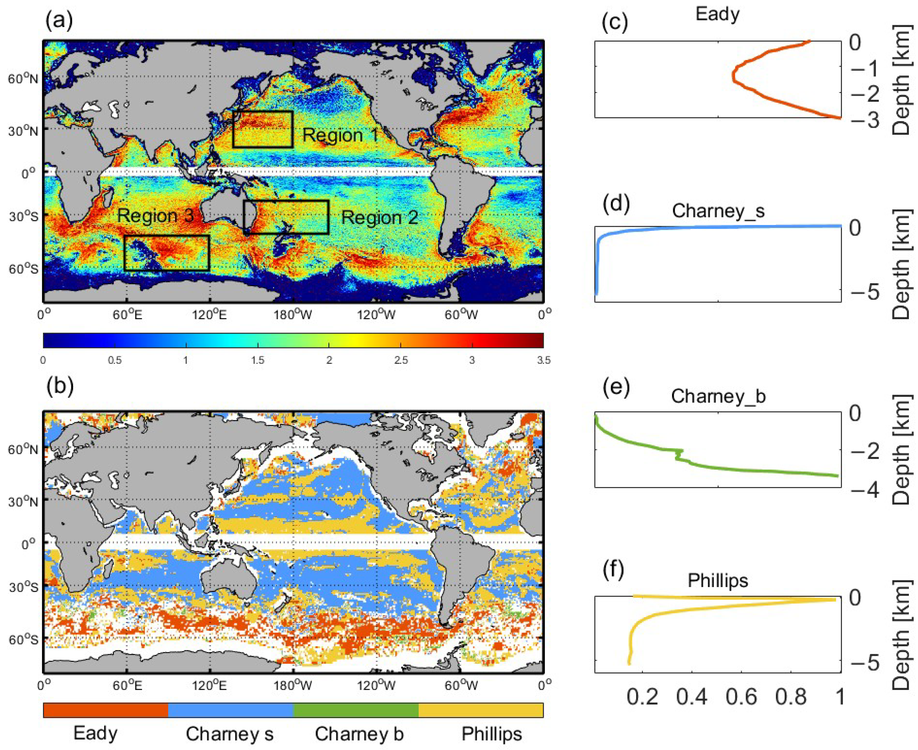
2.2.4. Baroclinic Instability Types and Their Potential Consequences

BCI is one of the important mechanisms for generating eddies, and because the vertical structure of the instability is basically unchanged during its nonlinear development [18], different types of instability develop to form eddies with different structures. The linear stability analysis method can be used to analyze various characteristics of BCI, including growth rate, spatial scale, and vertical structure [20,21]. According to the vertical structure, the BCI can be roughly classified into four types: (i) Eady-type, in which surface and bottom amplitudes are large, intermediate amplitudes are small, surface and bottom amplitudes tend to decay toward the middle, and the minimum amplitude is more than 0.3 (Figure 1c); (ii) Charney_s-type, in which surface amplitude is the largest, and it decays toward the bottom (Figure 1d); (iii) Charney_b-type, in which bottom amplitude is the largest, and it decays toward the surface (Figure 1e); and (iv) Phillips-type, in which subsurface amplitude is the largest and attenuates toward the surface and bottom (Figure 1f). Different kinds of BCI can predict different kinds of eddies, for example, Charney_s-type with the largest surface amplitude predicts surface-intensified eddies, Phillips-type with the largest subsurface amplitude predicts subsurface-intensified eddies, Charney_b-type with the largest bottom amplitude predicts bottom-intensified eddies, and Eady-type predicts surface- and bottom-intensified eddies.

This study firstly normalizes the vertical structure of the global eddies, where there is a wide distribution of three types of BCI, Charney_s, Phillips, and Eady, with Charney_s accounting for the largest share. Due to the differences in the number, size, and intensity of eddies, etc., the vertical signals that relate to other types of BCI may be obscured on a global scale. Therefore, considering the spatial distributions of EKE and BCI types (Figure 1a,b), we chose three typical regions that are rich in eddy activity and dominated by different types of BCI to investigate the similarities and differences in the evolution of these eddies’ properties and vertical structures. The study regions from north to south are as follows: the Northwest Pacific Ocean (20–42°N, 135–180°E), showcasing Phillips-type and Charney_s-type (hereinafter called Phillips + Charney_s-type) BCIs with seasonal variations; the midlatitude region of the South Pacific Ocean (20–40°S, 140°E–160°W), dominated by Charney_s-type BCI; and a specific portion of the Antarctic Circumpolar Current (40–60°S, 60–120°E), displaying Eady-type BCI.

It should be noted that in the real ocean, several types of instability usually coexist and interconvert under certain conditions, which means that the dominance of a particular BCI does not imply a prediction of the type of eddies that will be generated in the region as a whole. For example, in Region 2, the eddies here are dominated by Charney_s type BCI, but this does not mean that all the eddies here are surface-intensified; it is only after a sufficient number of statistical averages that the normalized structure shows the result of surface-intensified. Our results are also an analysis of the eddy structure in the sense of statistical averaging, which is not applicable to all eddies in the region.

3. Results

We identified and tracked mesoscale eddies globally, capturing a total of 228,393 cyclonic eddies (CEs) and 210,659 anticyclonic eddies (AEs). It is evident that mesoscale eddies are mainly distributed in the midlatitude regions, while in high-latitude regions, the presence of ice caps hinders eddy detection (Figure 2). Moreover, it can be observed that eddy activities are more prevalent along the east and west boundaries of the oceans than in the open ocean.

We examined the main properties of global mesoscale eddies, namely, their radius, amplitude, and EKE, in relation to lifespan (Figure 3). To account for differences in the eddies’ lifespans, each eddy was normalized to a range of 0–1, allowing for an evaluation of attribute evolution across all eddies. The properties of eddies experience three distinct periods over their lifespan: growth, stabilization, and decay. The growth and decay periods each account for 20% of an eddy’s lifespan, while the stabilization period falls between them. This finding aligns with previous studies [24,25,26,51]. Specifically, during the first 20% of an eddy’s lifespan, its radius, amplitude, and EKE increase. During the middle 60%, the eddy remains stable, while it decreases during the last 20% of its lifespan. Consequently, we selected the growth period (the first 20%), the decay period (the last 20%), and the middle part of the stabilization period (40–60%) as representative stages for studying the eddy’s evolution.

3.1. Evolutionary Characteristics of the Vertical Structure of Global Eddies

Figure 4 illustrates the vertical structure of worldwide CEs and AEs concerning potential temperature anomalies. The normalized structure of the global eddies is a single-core structure, with a core depth of about 50–300 m. This indicates that the surface eddies, corresponding to the Charney_s-type BCI, dominate the global ocean. Interestingly, for both CEs (the upper row of Figure 4) and AEs (the lower row of Figure 4), during different lifespan periods, there are apparent variations in the location and strength of their cores based on central potential temperature anomaly. From eddies’ growth to stabilization, the eddy-induced anomaly enhances and mainly spreads vertically, showing a trend of increasing with depth. For CEs, the core cools by 0.15 °C, and the maximum depth of eddy influence (based on the anomaly being equal to 0.2) deepens from 490 m to 650 m; simultaneously, the depth induced by AEs increases from 560 m to 720 m, and the core warms by 0.20 °C. The vertical process can also be seen from the average vertical profiles in Figure 5a–d. During the periods from eddies’ stabilization to decay, the eddy-induced potential temperature anomaly exhibits clear horizontal spread, causing the influence range to expand and ultimately resulting in a weakening of the eddy core. Additionally, compared with the global average temperature gradient profiles obtained from Argo profiles (Figure 5e), we found that the core of an eddy-induced anomaly is usually situated below the seasonal thermocline, which is discussed later in this article. It should be noted that our analyses are performed in vertical depth coordinates and do not account for the movements of isopycnals that may cause the structure of eddies to naturally shift up and down. This possible error has not been ruled out in this paper, and its impact needs further attention.

3.2. Basic Properties of Different Types of Eddies and Their Evolutionary Characteristics

The statistics for eddy identification are displayed in

Table 1. Information on the number and properties of eddies in the three selected regions.

Mean Properties	Region 1		Region 2		Region 3
	CEs	AEs	CEs	AEs	CEs	AEs
Number of eddies	5965	5852	9396	8960	6696	6007
Lifetime (days)	87	95	48	54	74	75
Radius (km)	67.55	72.65	56.97	60.63	49.31	54.66
Amplitude (cm)	9.63	9.76	5.55	6.01	9.99	9.52
Translation speed (km/day)	2.7	2.5	1.9	1.9	2.4	2.3

. The Kuroshio Extension makes up most of Region 1, and the type of BCI in this region takes the current axis as the boundary, with Phillips-type BCI south of the current axis and Charney_s-type BCI north of the current axis, respectively, whose specific boundaries have a north–south shift with seasons [23]. A total of 5965 CEs and 5852 AEs are identified in this region, and the average lifetime of AEs (95 days) is larger than that of CEs (87 days). The eddies here are the largest in radius and translation speed. In Region 2, Charney_s-type BCI dominates, which corresponds to surface eddies. Region 2 has the largest number of identified eddies, with 9396 CEs and 8960 AEs. However, the eddies here are relatively weaker, with amplitudes (only about 6 cm) and translation speed (1.9 km/day) significantly lower than those in the other two regions because of the weak current and lack of oceanic environment for strong eddy generation and propagation. Region 3 is dominated by the Eady-type BCI, corresponding to the surface- and bottom-intensified structure of the eddies. Eddies in this region have the smallest radius (about 50 km) due to the highest latitude, and their lifetimes are shorter than those in the other regions. However, due to the presence of the Antarctic Circumpolar Current (ACC), their amplitude and EKE are larger.

To further understand their variations with lifespan, we produced the composite mean properties during the evolution of the eddies in the study regions (Figure 6). The overall trend of properties in each region is similar to that of global eddies (see Figure 3). It also can be divided into three periods: growth, stabilization, and decay. It is observed that CEs have a smaller radius and larger EKE than AEs in all regions, whereas the magnitude of amplitude shows diversity. In Region 1, compared with AEs, CEs have a similar amplitude but a smaller radius after their growth period, which results in the EKE of CEs being significantly higher than that of AEs. Among the three regions, as eddies evolve, the amplitude of eddies in Region 2 is the smallest, leading to the smallest EKE. Moreover, because AEs have a larger amplitude and radius than CEs, the EKE of AEs and CEs here are very close. The eddies in Region 3 have the highest latitude, causing the eddies to have the smallest radius and to start to experience a decrease in amplitude and EKE earlier. Additionally, CEs in this region exhibit a larger amplitude than AEs.

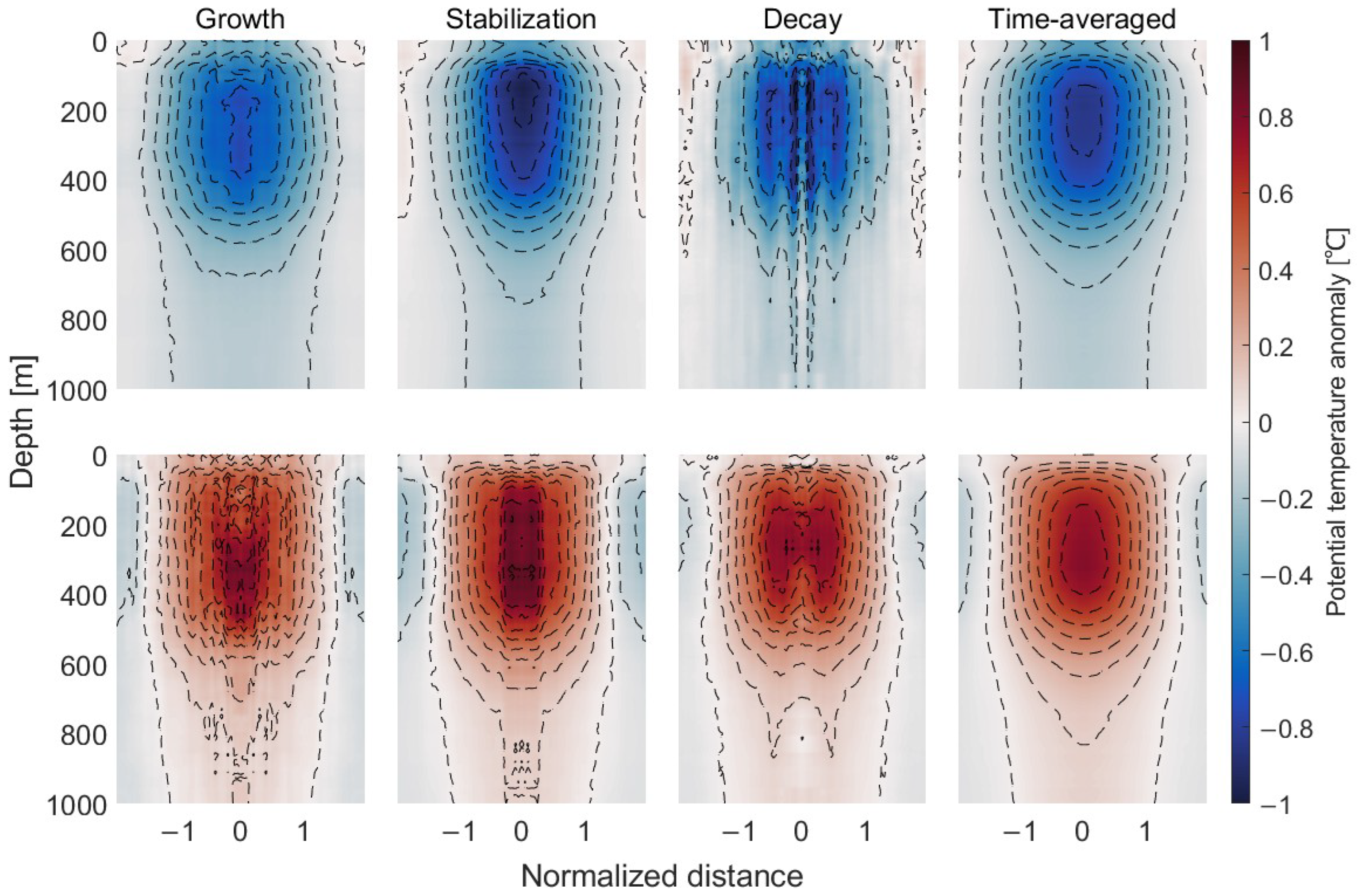
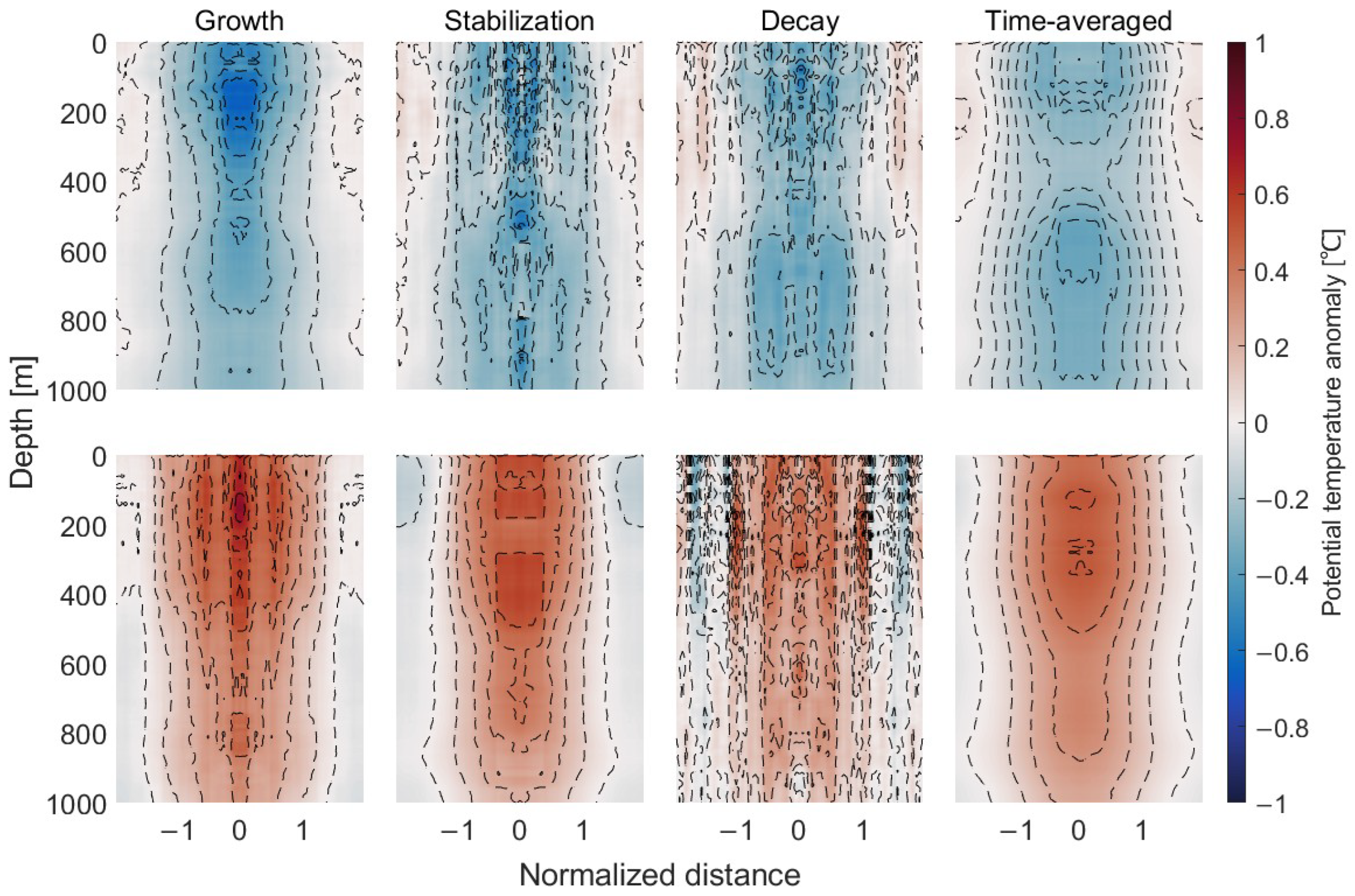
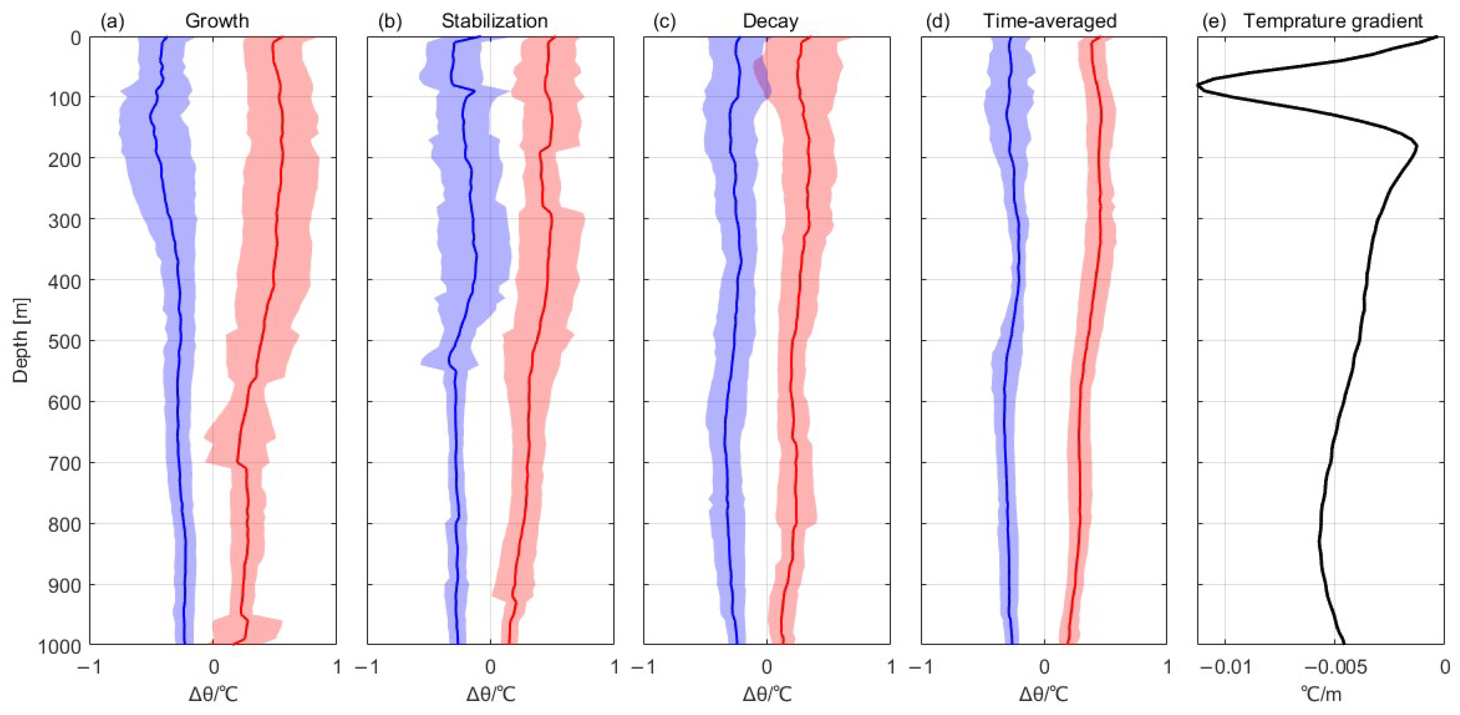
3.3. Evolutionary Characteristics of the Vertical Structure of Different Types of Eddies

Figure 7, Figure 8, Figure 9, Figure 10, Figure 11 and Figure 12 depict the evolution of vertical structures of CEs and AEs in Regions 1–3. In Region 1, the structures of AEs and CEs differ significantly due to different types of BCI on either side of the Kuroshio Current axis. CEs are primarily found on the south of the Kuroshio Current axis, which is dominated by Phillips-type BCI; AEs are most often located on the north of the Kuroshio Current axis, which is dominated by Charney_s-type BCI [23]. As Figure 7 shows, CEs exhibit a clear double-core structure, with the two cores positioned at approximately 100 m and 400 m. The core is well preserved throughout the entire lifespan with no discernible variance in its location and the intensity of the central temperature anomaly, maintaining a strong central temperature anomaly. Additionally, the vertical spread of the eddy-induced anomaly is more evident from the periods of stabilization to decay than that from the periods of growth to stabilization.

Different from CEs, AEs have a single-core structure with a core located at a depth of 50–300 m as a whole. Surprisingly, as they evolve, significant variations in their vertical structure occur which differ from both local CEs and global AEs. During the growth period, there is an anomalous cold core at a depth of 400–700 m, which is highly distinctive for AEs. In addition, a dual-core structure is found at depths of 100 m and 250 m above the anomalous cold core. The subsurface warm core and anomalous cold core share the same radius. Itoh and Yasuda (2010) [52] found that the cold water mass in the Okhotsk Sea moves southward and intrudes into the AEs on the west side of the Kuroshio Extension. Combined with our analysis, it is evident that the southward intrusion of the Okhotsk cold water mass primarily impacts the structure of the AEs during their growth period, which seems to produce numerous subsurface cold-core AEs due to the instability process ranging from 400 m to 700 m. This unique generation mechanism of AEs in this region leads to significant differences in the evolution of their vertical structure compared to the other two regions. Furthermore, due to the intensive temperature contrast between the upper and deeper water, heat exchange is more active, with vertical heat advection being stronger than in other regions for AEs in their growth to stabilization period. This generates a double-core structure during stabilization, and subsequently, it becomes a single-core structure under geostrophic adjustment. During the decay period, the center of AEs even has zero and partially negative values, indicating greater decay at the eddy core. Section 4 elaborates on the reason for the gradual adjustment of AEs to a single-core structure near 200 m during the evolution process.

To further quantify the vertical structure evolution of the eddies, we plotted the vertical profile of the potential temperature anomaly (Figure 8). From the mean potential temperature contours, AEs are generated with a three-core structure in which the cold core is located below the two warm cores; then, the warm cores expand vertically to create a dual-core structure during the stabilization period. Finally, they merge as a single-core structure and gradually dissipate. The CEs, on the other hand, have an obvious dual-core structure, and the intensity changes slightly during the evolution process, with the maximum anomaly of the cold core in the upper layer weakening from −1.22 °C to −1.14 °C, and the depth deepens from 110 m to 140 m; the maximum anomaly of the lower cold core is strengthened from −0.86 °C to −0.88 °C, and the depth decreases from 410 m to 390 m. Combining the changes of the AEs and CEs, we can see that CEs in this area have a tendency to adjust to the intermediate depth during the evolution process, and combined with the data of the mean temperature gradient profiles in this area (Figure 8e), we can speculate that the core of the eddy propagates to the intermediate depths of the seasonal thermocline and the permanent thermocline. A gradient threshold of −0.05 °C/m is chosen, and the anomalous strength of the CEs at 50 m, the intermediate depth of the seasonal thermocline, is weakened from −0.98 °C to −0.67 °C, and that of the AEs from 1.13 °C to 0.49 °C. The anomalous strength of the CEs at 250 m, the depth of the weakest gradient, is strengthened from −0.78 °C to −0.79 °C, and that of the AEs from 0.68 °C to 0.76 °C, showing that the evolution of the eddy core intensity at different depths is correlated with the local stratification conditions. The difference in the evolution of the AEs and CEs may be due to the dominance of different BCI structures; eddies generated by subsurface-intensified Phillips-type BCI have better retention in evolution, while eddies generated by surface-intensified Charney_s-type BCI tend to form a single-core structure in evolution, adjusting to decay in the intermediate depth range between the seasonal thermocline and the permanent thermocline.

In Region 2, the structures of potential temperature anomalies inside CEs and AEs are relatively similar, showing a surface-intensified structure corresponding to the Charney_s-type BCI (Figure 9). The overall structure and that of different periods are highly consistent: all are single-core structures with core depths near 200 m depth. The intensity evolution process of the AEs and CEs in this region is relatively ordinary, with the maximum anomaly value of AEs increasing from 0.62 °C to 0.70 °C from the growth period to the stabilization period and then weakening to 0.66 °C from the stabilization period to the decay period. CEs have a similar evolutionary process. In terms of stratification conditions (Figure 10e), this region has both a seasonal thermocline and a permanent thermocline, and in the seasonal thermocline with a strong vertical gradient, taken at a depth of 60 m, the anomalous strength of the CEs weakens from −0.46 °C to −0.37 °C, while the anomalous strength of the AEs weakens from 0.38 °C to 0.34 °C. By contrast, the anomalous strength of the CEs at 180 m, the weakest depth of the gradient, strengthens from −0.62 °C to −0.67 °C, and that of the AEs strengthens from 0.53 °C to 0.62 °C. It is possible to find that the evolutionary tendency of the strength of the eddies dominated by the Charney_s-type BCI in Region 2 is similarly correlated with the stratification of local conditions.

The dominant type of BCI in Region 3 is Eady, and its vertical structure is intensified on the surface and bottom layers. As we can see from Figure 11, the vertical structure of the CEs in this region has a cold core near the surface of 200 m, which evolves during its lifespan in a similar way to the surface eddies, generating spread in the vertical direction first and then in the horizontal direction. One special characteristic of eddies here is that the radius does not decrease as expected but increases slightly below 400 m depth. Although the intensity of the deeper anomaly is not as strong as the surface core, it does not decay significantly with depth. This structure could correspond to the bottom-intensified Eady-type BCI; however, due to the diverse depths at different locations, the deeper anomaly cannot form an eddy core at a uniform depth. Compared with CEs, AEs are similar as a whole, although the anomaly is stronger in the surface layer. Despite some errors resulting from insufficient in situ observations, as seen from the existing results, we find a special characteristic where, from the periods of stabilization to decay, the surface core exhibits a tendency to be adjusted to a depth of 150 m and becomes stronger. This process requires further study.

In general, the eddies’ vertical structures and their evolution corresponding to various types of BCI are markedly distinct. The surface-intensified eddies corresponding to Charney_s-type BCI have a single-core structure, with the core at a depth of 200 m; the surface- and bottom-intensified eddies corresponding to the Eady-type BCI have a dual-core structure, with the cores distributed around 150 m and 600 m, respectively, and the upper core is stronger than the deeper core. The eddies corresponding to Phillips-type and Charney_s-type BCIs show both surface- and subsurface-intensified eddies, with double cores appearing near the depths of 100 m and 400 m, respectively. In terms of the evolution process, the surface-intensified eddies corresponding to the Charney_s-type BCI and the surface-intensified part of the eddies corresponding to the Eady-type BCI both have vertical spread from the periods of growth to stabilization, which can be clearly explained from the perspective of thermal diffusion or energy diffusion. However, from the periods of stabilization to decay, the surface cores are concentrated at a certain depth and gradually dissipate. This potential mechanism currently lacks sufficient explanation. We present the average temperature profiles obtained from Argo profiles in study regions and identify their thermocline by the gradient method. This suggests that the depth at which the surface core concentrates during the decay period is clearly correlated with the local oceanic stratification, which is discussed in more detail in Section 4.

For the subsurface structure corresponding to the Phillips-type BCI and the bottom-intensified part of the Eady-type BCI, there is no apparent spread and decay process during the eddies’ lifespan. We hypothesize that the surface core has stronger decay, while the subsurface and bottom cores have greater retention, resulting in a significant decay of nonsurface eddy cores only after the surface core is fully dissipated. However, it should be noted that the identification of mesoscale eddies primarily relies on surface-layer data, and the subsurface and bottom cores cannot be effectively observed once the surface core dissipates. Due to the challenge of accessing data below the sea surface, it is necessary to conduct further investigation into the decay process of subsurface and bottom structures inside eddies.

4. Discussion

We list the mean values of potential temperature anomalies within a radius at different depths for different periods of the eddy (

Table 2. Mean values of eddy-induced potential temperature anomalies at different depths in three regions.

	Depth (m)	CEs			AEs
Region 1	20	−0.68	−0.48	−0.42	0.67	0.21	0.20
	50	−0.98	−0.77	−0.67	1.13	0.49	0.49
	250	−0.78	−0.73	−0.79	0.68	0.58	0.76
	500	−0.73	−0.71	−0.60	0.01	0.44	0.23
Region 2	20	−0.37	−0.36	−0.32	0.23	0.15	0.11
	60	−0.46	−0.38	−0.37	0.38	0.39	0.34
	180	−0.62	−0.78	−0.67	0.53	0.68	0.62
	400	−0.58	−0.67	−0.57	0.58	0.65	0.56
Region 3	20	−0.40	−0.29	−0.24	0.48	0.46	0.27
	80	−0.39	−0.31	−0.22	0.53	0.44	0.24
	180	−0.35	−0.21	−0.28	0.54	0.34	0.48
	800	−0.26	−0.25	−0.24	0.28	0.27	0.24

), which to some extent can reflect the structure and evolution of the eddy, as well as the decay of the eddy at different depths. Regarding the selection of depths, the mixed layer, the seasonal thermocline, the depth range of the weakest gradient, and the permanent thermocline were chosen for different regions in the hope of exploring the effect of the vertical gradient on eddy decay.

A comprehensive analysis of the evolution of the potential temperature anomaly in the seasonal thermocline in the three regions (at depths of 50 m, 60 m, and 80 m) reveals that the mean potential temperature anomaly at this depth undergoes a continuous weakening process from the growth period to the decay period. The values during the decay period are usually only about half as strong as the values during the growth period, which shows stronger decay compared to other depths, especially the depth range of the weakest gradient. The evolution of the mean potential temperature anomaly at the depth of the permanent thermocline also shares similarities with the seasonal thermocline, showing a rapid weakening from the stabilization to the decay period, whereas the stabilization or even enhancement from the growth to the stabilization period differs from that of the seasonal thermocline and is speculated to be due to the vertical spread of an eddy-induced potential temperature anomaly from the growth to the stabilization period. We believe that the decay of eddies is intensified in the depth range with stronger vertical gradients. Meanwhile, the horizontal shear caused by the propagation of the eddies also accelerates the decay process. This further confirms that during the evolution of eddies, their surface anomalous structure found in various regions tends to concentrate towards the depths with the weakest vertical gradients during the evolution of eddies, because decay is stronger at depths with large vertical gradients and weaker at depths with smaller gradients.

It is found that the mean potential temperature anomaly in the mixed layer (considering a depth of 20 m) is weak and also shows a rapid decrease. This is because the seasonal thermocline acts as a barrier to some extent, leading to the potential temperature anomaly almost dissipating in the thermocline. As a result, it is hard for the anomaly to reach the mixed layer. Moreover, a small amount of the potential temperature anomaly that can spread into the mixed layer is also dissipated rapidly due to the effect of wind stress, waves, etc. [30]. This also explains why the surface cores of eddies in each region are located below the thermocline, while the potential temperature anomaly at the sea surface is very small. It should be noted that the structure of the eddy-induced potential temperature anomaly based on the composite analysis in this paper only gives the conclusion that the vertical gradient affects the eddy decay rate from the observation but lacks the analysis of the dynamical mechanism, which may require further verification of the in situ observation data, and at the same time, the selected thermocline, which is not a strictly defined thermocline, only represents part of the strongest depth range of the vertical gradient.

Comparing the structure of eddy-induced potential temperature anomalies in the three regions, it is found that there are obvious differences in their structures. In Region 1, the dominant BCI type in this region varies seasonally between the two types of Charney_s and Phillips, and the main reason for the variations is the changes in the seasonally induced stratification conditions [53]; while the CEs here show surface- and subsurface-intensified types and their depths and structures are consistent with the BCI type here, the AEs here have a special structure due to the invasion of the Okhotsk cold water mass in the growth period and lead to a completely different evolutionary process from the CEs. This partly explains the limitation of the BCI type in predicting the structure of eddies due to its inability to predict the structure of eddies generated by a similar process. In Region 2, the dominant BCI type is Charney_s type, and the CEs and AEs in this region have similar structures and are located at similar depths with similar evolutionary processes. However, comparing the structure of the global mesoscale eddy (Figure 4), it is found that the main difference lies in the core depths, which are significantly deeper in Region 2, which to some extent illustrates that the structures of the eddies corresponding to the same type of BCI are not identical and may be altered depending on varying background ocean states. The influence of varying background ocean states on the structure of the eddy and the specific mechanism of their influence need to be revealed in future work. The dominant BCI type of Region 3 is Eady-type, which corresponds to the surface- and bottom-intensified structure and which is reflected in the vertical structure shown in Figure 11, and two eddy cores exist at the depths of 200 m and 600 m downward extension; the depth of 1000 m was chosen for this study to be consistent with that of the global and other regions’ study, but based on the previous studies, the eddy in the ACC region will be affected by the merging effect [26] and will affect deeper, as it can exist at a maximum depth of 2000 m. The eddy-induced potential temperature anomaly at 1000 m does not have obvious attenuation, as can be seen in Figure 11, and a deeper depth is needed to obtain the complete structure and evolution of the eddy to carry out further studies in this region.

5. Summary and Conclusions

In this study, we analyzed the evolution of global eddies as well as different types of eddies based on BCIs by using satellite altimetry, Argo profiles, and climatology data. The results show that the global eddies are dominated by the surface eddies corresponding to Charney_s-type BCI, and their evolution can be basically divided into three main periods, which are the growth, stabilization, and decay periods. The main variation in the evolution from the periods of growth to stabilization is the vertical spread of anomalous structures, represented by the deepening of influence depth; and from the periods of stabilization to decay, the main variations are the horizontal spread and the weakening of anomalous intensity, represented by an increase in the range of influence and a decrease in the intensity of influence.

Based on the global spatial distribution of the types of BCI and EKE, we selected three typical ocean regions, namely, the Northwest Pacific Ocean (dominated by Phillips-type and Charney_s-type BCIs), the midlatitude region of the South Pacific Ocean (dominated by Charney_s-type BCI), and a part of the Southern Ocean (dominated by Eady-type BCIs), for further investigation of the evolution of different types of eddies. The evolution of the basic properties of different types of eddies is similar to that of global eddies, as the lifespan can be divided into three main stages. However, the vertical structure and its evolution of different types of eddies are significantly different: the Charney_s-type BCI corresponds to single-core surface-intensified eddies with a core at a depth of 200 m; the Eady-type BCI corresponds to dual-core surface- and bottom-intensified eddies, with cores at around 150 m and 600 m, respectively; and the Phillips + Charney_s-type BCI corresponds to eddies that exhibit both surface- and subsurface-intensified eddy structures, with dual cores distributed near the depths of 100 m and 400 m, respectively. In particular, the southward intrusion of the Okhotsk cold water mass in Region 1 may contribute to the formation of AEs’ anomalous structure, leading to distinct structure and evolution from other regions. The surface-intensified eddies corresponding to Charney_s-type BCI and the surface-intensified part of the eddies corresponding to Eady-type BCIs undergo spread in both the vertical and horizontal directions, which is similar to that of global eddies. On the other hand, the subsurface-intensified eddies corresponding to Phillips-type BCI and the bottom-intensified part of the eddies corresponding to Eady-type BCI undergo a significantly slower decay process than that of the surface-intensified eddies. Since the surface structure of eddies has already disappeared when the subsurface and bottom cores start to dissipate, and eddies are identified based on the surface data, the evolution of the subsurface- and bottom-intensified eddies remains to be further explored in future work.

Additionally, we examined the impact of oceanic local stratification structure on eddy evolution by analyzing the eddy-induced potential temperature anomaly, as we found a significant correlation between the depth of eddies’ surface core and the intensity of local stratification during their decay period. An increase in the vertical gradient intensifies eddies’ decay, causing the eddy-induced anomaly to concentrate at depths where the vertical gradient is the weakest during their evolution. Due to the thermocline acting as a barrier and the effects of winds and waves amplifying the decay, eddies tend to have weak surface structures. This explains not only why the surface core of eddies is usually weak but also why it is located underneath the thermocline. It should be noted that the current conclusions regarding the vertical gradient and eddy decay are based on the description of the normalized structure, which lacks the support of the dynamical mechanism and needs to be verified with more data and support from future work.

Regarding the predictability of the BCI type on eddies, the vertical structure of surface- and subsurface-intensified eddies show some similarity but are not strictly the same, but the bottom-intensified eddies, for which there are not enough data to reveal the structure, still need more evidence to verify the predictability of the BCI type. Regarding the AEs in Region 1, the invasion of the cold water mass leads to a structure that is very far from that of the BCI type. For the surface-intensified eddies in Region 2, their deeper depths indicate that the BCI type is also modulated by varying background ocean states. The evidence suggests that the BCI has many limitations in its ability to predict eddy structure and that a more nuanced relationship between the BCI and mesoscale eddies needs to be addressed by further work.

References

1. Chelton, D.B.; Schlax, M.G.; Samelson, R.M. Global observations of nonlinear mesoscale eddies. Prog. Oceanogr. 2011, 91, 167–216. [Google Scholar] [CrossRef]
2. Chelton, D.B.; Schlax, M.G.; Samelson, R.M.; de Szoeke, R.A. Global observations of large oceanic eddies. Geophys. Res. Lett. 2007, 34, L15606. [Google Scholar] [CrossRef]
3. Wunsch, C.; Ferrari, R. Vertical mixing, energy and the general circulation of the oceans. Annu. Rev. Fluid Mech. 2004, 36, 281–314. [Google Scholar] [CrossRef]
4. Chen, G.; Wang, D.; Hou, Y. The features and interannual variability mechanism of mesoscale eddies in the Bay of Bengal. Cont. Shelf Res. 2012, 47, 178–185. [Google Scholar] [CrossRef]
5. Dong, C.; McWilliams, J.C.; Liu, Y.; Chen, D. Global heat and salt transports by eddy movement. Nat. Commun. 2014, 5, 3294. [Google Scholar] [CrossRef] [PubMed]
6. Ning, J.; Chen, K.; Gaube, P. Diverse variability of surface chlorophyll during the evolution of Gulf Stream rings. Geophys. Res. Lett. 2021, 48, e2020GL091461. [Google Scholar] [CrossRef]
7. Gaube, P.; Chelton, D.B.; Samelson, R.M.; Schlax, M.G.; O’neill, L.W. Satellite observations of mesoscale eddy-induced Ekman pumping. J. Phys. Oceanogr. 2015, 45, 104–132. [Google Scholar] [CrossRef]
8. Hausmann, U.; Czaja, A. The observed signature of mesoscale eddies in sea surface temperature and the associated heat transport. Deep. Sea Res. Part I Oceanogr. Res. Pap. 2012, 70, 60–72. [Google Scholar] [CrossRef]
9. Qiu, B.; Chen, S. Variability of the Kuroshio Extension jet, recirculation gyre, and mesoscale eddies on decadal time scales. J. Phys. Oceanogr. 2005, 35, 2090–2103. [Google Scholar] [CrossRef]
10. Zhang, Z.; Wang, W.; Qiu, B. Oceanic mass transport by mesoscale eddies. Science 2014, 345, 322–324. [Google Scholar] [CrossRef]
11. Sun, W.; Dong, C.; Tan, W.; Liu, Y.; He, Y.; Wang, J. Vertical structure anomalies of oceanic eddies and eddy-induced transports in the South China Sea. Remote Sens. 2018, 10, 795. [Google Scholar] [CrossRef]
12. Xu, G.; Dong, C.; Liu, Y.; Gaube, P.; Yang, J. Chlorophyll Rings around Ocean Eddies in the North Pacific. Sci. Rep. 2019, 9, 2019. [Google Scholar] [CrossRef] [PubMed]
13. Vallis, G.K. (Ed.) Atmospheric and Oceanic Fluid Dynamics; Cambridge University Press: Cambridge, UK, 2006; pp. 247–287. [Google Scholar]
14. Sun, W.; Yang, J.; Tan, W.; Liu, Y.; Zhao, B.; He, Y.; Dong, C. Eddy diffusivity and coherent mesoscale eddy analysis in the Southern Ocean. Acta Oceanol. Sin. 2021, 40, 1–16. [Google Scholar] [CrossRef]
15. Sun, W.; Dong, C. Isopycnal and diapycnal mixing parameterization schemes for submesoscale processes induced by mesoscale eddies. Deep. Sea Res. Part II Top. Stud. Oceanogr. 2022, 202, 105139. [Google Scholar] [CrossRef]
16. Gill, A.; Green, J.; Simmons, A. Energy partition in the large-scale ocean circulation and the production of mid-ocean eddies. Deep. Sea Res. Oceanogr. Abstr. 1974, 21, 499–528. [Google Scholar] [CrossRef]
17. Pedlosky, J. Geophysical Fluid Dynamics, 2nd ed.; Springer: Berlin, Germany, 1987. [Google Scholar]
18. Roullet, G.; McWilliams, J.C.; Capet, X.; Molemaker, M.J. Properties of steady geostrophic turbulence with isopycnal outcropping. J. Phys. Oceanogr. 2012, 42, 18–38. [Google Scholar] [CrossRef]
19. Venaille, A.; Vallis, G.K.; Smith, K.S. Baroclinic turbulence in the ocean: Analysis with primitive equation and quasigeostrophic simulations. J. Phys. Oceanogr. 2015, 41, 1605–1623. [Google Scholar] [CrossRef]
20. Smith, K.S. The geography of linear baroclinic instability in Earth’s oceans. J. Mar. Res. 2007, 65, 655–683. [Google Scholar] [CrossRef]
21. Tulloch, R.; Marshall, J.; Hill, C.; Smith, K.S. Scales, growth rates, and spectral fluxes of baroclinic instability in the ocean. J. Phys. Oceanogr. 2011, 41, 1057–1076. [Google Scholar] [CrossRef]
22. Beckmann, A. Vertical Structure of Midlatitude Mesoscale Instabilities. J. Phys. Oceanogr. 1988, 18, 1354–1371. [Google Scholar] [CrossRef]
23. Feng, L.; Liu, C.; Köhl, A.; Stammer, D.; Wang, F. Four types of baroclinic instability waves in the global oceans and the implications for the vertical structure of mesoscale eddies. J. Geophys. Res. Ocean. 2021, 126, e2020JC016966. [Google Scholar] [CrossRef]
24. Liu, Y.; Dong, C.; Guan, Y.; Chen, D.; McWilliams, J.; Nencioli, F. Eddy analysis in the subtropical zonal band of the North Pacific Ocean. Deep. Sea Res. Part I Oceanogr. Res. Pap. 2012, 68, 54–67. [Google Scholar] [CrossRef]
25. Yang, G.; Wang, F.; Li, Y.; Lin, P. Mesoscale eddies in the northwestern subtropical Pacific Ocean: Statistical characteristics and three-dimensional structures. J. Geophys. Res. Ocean. 2013, 118, 1906–1925. [Google Scholar] [CrossRef]
26. Frenger, I.; Gruber, N.; Knutti, R.; Münnich, M. Southern Ocean eddy phenomenology. J. Geophys. Res.-Ocean. 2015, 120, 7413–7449. [Google Scholar] [CrossRef]
27. Zhang, Z.; Zhang, Y.; Wang, W.; Huang, R.X. Universal structure of mesoscale eddies in the ocean. Geophys. Res. Lett. 2013, 40, 3677–3681. [Google Scholar] [CrossRef]
28. Zhai, X.; Johnson, H.L.; Marshall, D.P. Significant sink of ocean-eddy energy near western boundaries. Nat. Geosci. 2010, 3, 608–612. [Google Scholar] [CrossRef]
29. Evans, D.G.; Frajka-Williams, E.E.; Garabato, A.C.N.; Polzin, K.L.; Forryan, A. Mesoscale eddy dissipation by a “zoo” of submesoscale processes at a western boundary. J. Geophys. Res. Ocean. 2020, 125, e2020JC016246. [Google Scholar] [CrossRef]
30. Dong, J.; Fox-Kemper, B.; Jing, Z.; Yang, Q.; Tian, J.; Dong, C. Turbulent Dissipation in the Surface Mixed Layer of an Anticyclonic Mesoscale Eddy in the South China Sea. Geophys. Res. Lett. 2022, 49, e2022GL100016. [Google Scholar] [CrossRef]
31. Le Traon, P.Y.; Nadal, F.; Ducet, N. An Improved Mapping Method of Multisatellite Altimeter Data. J. Atmos. Ocean. Technol. 1998, 15, 522–534. [Google Scholar] [CrossRef]
32. Nencioli, F.; Dong, C.; Dickey, T.; Washburn, L.; McWilliams, J.C. A vector geometry-based eddy detection algorithm and its application to a high-resolution numerical model product and high-frequency radar surface velocities in the Southern California Bight. J. Atmos. Ocean. Technol. 2010, 27, 564–579. [Google Scholar] [CrossRef]
33. Dong, C.; Mavor, T.; Nencioli, F.; Jiang, S.; Uchiyama, Y.; McWilliams, J.C.; Dickey, T.; Ondrusek, M.; Zhang, H.; Clark, D.K. An oceanic cyclonic eddy on the lee side of Lanai Island, Hawai’i. J. Geophys. Res. Earth Surf. 2009, 114, C10008. [Google Scholar] [CrossRef]
34. Dong, C.; Liu, Y.; Lumpkin, R.; Lankhorst, M.; Chen, D.; McWilliams, J.C.; Guan, Y. A Scheme to Identify Loops from Trajectories of Oceanic Surface Drifters: An Application in the Kuroshio Extension Region. J. Atmos. Ocean. Technol. 2011, 28, 1167–1176. [Google Scholar] [CrossRef]
35. Dong, C.; Lin, X.; Liu, Y.; Nencioli, F.; Chao, Y.; Guan, Y.; Chen, D.; Dickey, T.; McWilliams, J.C. Three-dimensional oceanic eddy analysis in the Southern California Bight from a numerical product. J. Geophys. Res. Ocean. 2012, 117, C00H14. [Google Scholar] [CrossRef]
36. Aguiar, A.C.B.; Peliz, Á.; Carton, X. A census of Meddies in a long-term high-resolution simulation. Prog. Oceanogr. 2013, 116, 80–94. [Google Scholar] [CrossRef]
37. Lin, X.; Dong, C.; Chen, D.; Liu, Y.; Yang, J.; Zou, B.; Guan, Y. Three-dimensional properties of mesoscale eddies in the South China Sea based on eddy-resolving model output. Deep. Sea Res. Part I Oceanogr. Res. Pap. 2015, 99, 46–64. [Google Scholar] [CrossRef]
38. Yang, X.; Xu, G.; Liu, Y.; Sun, W.; Xia, C.; Dong, C. Multi-source data analysis of mesoscale eddies and their effects on surface chlorophyll in the Bay of Bengal. Remote Sens. 2020, 12, 3485. [Google Scholar] [CrossRef]
39. Sun, W.; An, M.; Liu, J.; Liu, J.; Yang, J.; Tan, W.; Dong, C.; Liu, Y. Comparative analysis of four types of mesoscale eddies in the Kuroshio-Oyashio extension region. Front. Mar. Sci. 2022, 9, 984244. [Google Scholar] [CrossRef]
40. An, M.; Liu, J.; Liu, J.; Sun, W.; Yang, J.; Tan, W.; Liu, Y.; Sian, K.T.; Ji, J.; Dong, C. Comparative analysis of four types of mesoscale eddies in the north pacific subtropical countercurrent region—Part I spatial characteristics. Front. Mar. Sci. 2022, 9, 1004300. [Google Scholar] [CrossRef]
41. Dong, C.; Liu, L.; Nencioli, F.; Bethel, B.J.; Liu, Y.; Xu, G.; Ma, J.; Ji, J.; Sun, W.; Shan, H.; et al. The near-global ocean mesoscale eddy atmospheric-oceanic-biological interaction observational dataset. Sci. Data 2022, 9, 436. [Google Scholar] [CrossRef]
42. Chaigneau, A.; Le Texier, M.; Eldin, G.; Grados, C.; Pizarro, O. Vertical structure of mesoscale eddies in the eastern South Pacific Ocean: A composite analysis from altimetry and Argo profiling floats. J. Geophys. Res. Earth Surf. 2011, 116, C11025. [Google Scholar] [CrossRef]
43. Yang, G.; Yu, W.; Yuan, Y.; Zhao, X.; Wang, F.; Chen, G.; Liu, L.; Duan, Y. Characteristics, vertical structures, and heat/salt transports of mesoscale eddies in the southeastern tropical Indian Ocean. J. Geophys. Res. Ocean. 2015, 120, 6733–6750. [Google Scholar] [CrossRef]
44. Sun, W.; Dong, C.; Wang, R.; Liu, Y.; Yu, K. Vertical structure anomalies of oceanic eddies in the Kuroshio Extension region. J. Geophys. Res. 2017, 122, 1476–1496. [Google Scholar] [CrossRef]
45. Lukas, R.; Lindstrom, E. The mixed layer of the western equatorial Pacific Ocean. J. Geophys. Res. Atmos. 1991, 96, 3343–3357. [Google Scholar] [CrossRef]
46. Dong, S.; Sprintall, J.; Gille, S.T.; Talley, L. Southern Ocean mixed-layer depth from Argo float profiles. J. Geophys. Res. Earth Surf. 2008, 113, C06013. [Google Scholar] [CrossRef]
47. Defant, A. Physical Oceanography; Pergamon: London, UK, 1961; Volume 1. [Google Scholar]
48. Wyrtki, K. The thermal structure of the eastern Pacific Ocean. Dstch. Hydrogr. Zeit. Suppl. Ser. A 1964, 8, 6–84. [Google Scholar]
49. Chu, P.C.; Liu, Q.Y.; Jia, Y.L.; Fan, C.W. Evidence of barrier layer in the Sulu and Celebes Seas. J. Phys. Oceanogr. 2002, 32, 3299–3309. [Google Scholar] [CrossRef]
50. Holte, J.; Talley, L. A new algorithm for finding mixed layer depths with applications to Argo data and subantarctic mode water formation. J. Atmos. Ocean. Technol. 2009, 26, 1920–1939. [Google Scholar] [CrossRef]
51. Samelson, R.M.; Schlax, M.G.; Chelton, D.B. Randomness, Symmetry, and Scaling of Mesoscale Eddy Life Cycles. J. Phys. Oceanogr. 2014, 44, 1012–1029. [Google Scholar] [CrossRef]
52. Itoh, S.; Yasuda, I. Water Mass Structure of Warm and Cold Anticyclonic Eddies in the Western Boundary Region of the Subarctic North Pacific. J. Phys. Oceanogr. 2010, 40, 2624–2642. [Google Scholar] [CrossRef]
53. Feng, L.; Liu, C.; Köhl, A.; Wang, F. Seasonality of four types of baroclinic instability in the global oceans. J. Geophys. Res. Ocean. 2022, 127, e2022JC018572. [Google Scholar] [CrossRef]
Figure 1. (a) Distribution of global ocean multiyear (1998–2021) mean surface eddy kinetic energy (in cm2/s2; data are logarithmically processed with a base of 10). (b) Global distribution of the types of BCI. The right column of subfigures are vertical profile of stream function of (c) Eady-type, (d) Charney_s-type, (e) Charney_b-type, and (f) Phillips-type BCI (Subfigures (bf) based on Feng et al., 2021 [23]).
Remotesensing 15 05730 g001
Figure 2. Global distribution of identified eddies for the period from 1998 to 2021.
Remotesensing 15 05730 g002
Figure 3. Variation in global eddies’ (a) radius, (b) amplitude, and (c) EKE with lifespan.
Remotesensing 15 05730 g003
Figure 4. Normalized structure of the potential temperature anomaly of the global CEs (upper row) and AEs (lower row); four columns from left to right show the normalized structure of the structure of the eddies’ growth period, stabilization period, decay period, and time-averaged period, respectively; and the horizontal axis is represented by the normalized eddy radius (R).
Remotesensing 15 05730 g004
Figure 5. Average vertical profiles of potential temperature anomaly of global cyclonic and anticyclonic eddies within a radius range. (ad) Vertical profiles of eddies’ growth, stabilization, and decay periods and time-averaged period, respectively. (e) Mean temperature gradient profile obtained from Argo profiles over the selected range. Blue and red lines relate to potential temperature anomaly and indicate CEs and AEs, respectively. Shaded area represents one standard deviation. Black line indicate mean temperature gradient profile.
Remotesensing 15 05730 g005
Figure 6. Evolution of the radius, amplitude, and EKE of mesoscale eddies in Regions 1–3. (Red and blue lines represent AEs and CEs, respectively; black lines represent their mean values).
Remotesensing 15 05730 g006
Figure 7. Normalized structure of potential temperature anomaly for the cyclonic (upper row) and anticyclonic (lower row) eddies in Region 1; four columns from left to right show the normalized structure of the eddies’ growth period, stabilization period, and decay period and the time-averaged period, respectively; the horizontal axis is represented by the normalized eddy radius (R).
Remotesensing 15 05730 g007
Figure 8. Average vertical profiles of potential temperature anomaly of the cyclonic and anticyclonic eddies in Region 1. (ad) Vertical profiles of eddies’ growth, stabilization, and decay periods and the time-averaged period, respectively. (e) Mean temperature gradient profile obtained from Argo profiles over Region 1. Blue and red lines relate to potential temperature anomaly and indicate CEs and AEs, respectively. Shaded area represents one standard deviation. Black line indicate mean temperature gradient profile.
Remotesensing 15 05730 g008
Figure 9. This figure is the same as Figure 7, except it shows the cyclonic and anticyclonic eddies in Region 2.
Remotesensing 15 05730 g009
Figure 10. This figure is the same as Figure 8, except it shows the cyclonic and anticyclonic eddies in Region 2.
Remotesensing 15 05730 g010
Figure 11. This figure is the same as Figure 7, except it shows the cyclonic and anticyclonic eddies in Region 3.
Remotesensing 15 05730 g011
Figure 12. This figure is the same as Figure 8, except it shows the cyclonic and anticyclonic eddies in Region 3.
Remotesensing 15 05730 g012