Communication

Sea Surface Height Wavenumber Spectrum from Airborne Interferometric Radar Altimeter

1
Key Laboratory of Ocean Observation and Forecasting, Key Laboratory of Ocean Circulation and Waves, Institute of Oceanology, Chinese Academy of Sciences, Qingdao 266071, China
2
Laoshan Laboratory, Qingdao 266373, China
3
Center for Ocean Mega-Science and Technology, Chinese Academy of Sciences, Qingdao 266071, China
4
University of Chinese Academy of Sciences, Beijing 100049, China
5
Beijing Institute of Radio Measurement, Beijing 100854, China
6
Marine Survey Research Center, First Institute of Oceanography, Ministry of Natural Resources, Qingdao 266061, China
7
Yantai Marine Center, Ministry of Natural Resources, Yantai 264006, China
*
Author to whom correspondence should be addressed.
These authors contributed equally to this work.
Remote Sens. 2024, 16(8), 1359; https://doi.org/10.3390/rs16081359
Submission received: 21 February 2024 / Revised: 4 April 2024 / Accepted: 9 April 2024 / Published: 12 April 2024
(This article belongs to the Special Issue Applications of Satellite Altimetry in Ocean Observation)

Abstract

:
The proposed “Guanlan” ocean science satellite, led by China’s Laoshan Laboratory, includes an interferometric radar altimeter (IRA) as a key payload. As an integral part of its development, an airborne IRA experiment was conducted on 6 November 2021, with a flight path of approximately 90 km in the South China Sea. This study investigates the IRA’s ability to observe ocean sea surface height (SSH) across scales ranging from meters to mesoscale. The sea surface height anomaly (SSHA) of the IRA is aligned with the SSHA of the AVISO at scales greater than 30 km, but also demonstrates the ability to capture small-scale SSHA changes in two dimensions. We analyzed wavenumber spectra of SSHA obtained from the airborne IRA, ICESat-2, and SARAL/AltiKa satellite for this region. The results show a good agreement in power spectral density (PSD) levels between ICESat-2, SARAL/AltiKa and IRA at scales larger than 30 km. Within the submesoscale range of 1–10 km, the IRA SSHA spectrum exhibits a distinctly negative slope and the lowest energy level. The minimum PSD level of the IRA fell in the range of 10−4–10−3 m2/cycle/km, at scales around 1 km, which is more than an order of magnitude lower than that of ICESat-2, forming a spectral gap that is in agreement with the theoretical expectation. Furthermore, IRA-derived wave direction and significant wave height matched well with the MFWAM wave data. The results of this study underscore the considerable potential of airborne IRA in capturing SSHA across a range of scales, from oceanic waves to submesoscale.

1. Introduction

Understanding ocean dynamics is critically dependent on accurate measurements of SSH variability. Satellite altimetry has become an essential tool for monitoring sea surface height variations and mapping ocean topography from space. While conventional radar satellite altimetry has proven effective in capturing mesoscale SSHA, accurately detecting submesoscale oceanic processes through satellite remote sensing remains a significant challenge [1,2,3].
Using an interferometric altimeter is a robust technique widely recognized for its ability to provide high-resolution and accurate estimations of sea surface elevations. The Surface Water and Ocean Topography (SWOT) satellite mission was designed to resolve SSHA at wavelengths down to ~15 km [4,5]. A recent study shows that SWOT’s 2 km2 data product appears to achieve about three times better resolution [6]. The 2 km data product is derived from 250 m native grid data. It is worth noting that smoothing and other data processing operations can have an effect on signals at larger scales. A more rigorous analysis of KaRIn’s signal-to-noise performance, which involves many complicated factors, is still under study.
Airborne IRA has the advantage of being close to the sea surface and having a strong echo signal. The airborne IRA also has the capability to monitor two-dimensional (2D) SSHA. If it proves successful in resolving SSHA at scales below 15 km, a task that presents significant challenges for satellite-based observations, it will offer a wide spectrum of potential applications. AirSWOT is designed to perform interferometric measurements similar to those performed by SWOT in space using the Ka-band SWOT Phenomenology Airborne Radar. AirSWOT’s high-precision measurements have proven to be valuable for hydrologic analysis, flood modeling studies, and river discharge estimation [7,8]. As part of the efforts for China’s future IRA satellite altimeter missions for monitoring ocean surface topography, an airborne interferometric altimeter (Airborne IRA) has been made by the Beijing Institute of Radio Measurement. The airborne IRA data were studied in three previous experiments: on 31 March 2019, in the Xiaomaidao Sea Area in Qingdao, China [9,10,11]; on 16 November 2020, in the Rizhao Sea Area, China [11,12,13]; and on 6 November 2021, in the South China Sea [11]. The SSHA reconstruction from the airborne IRA was improved by applying a multichannel likelihood method [13]. The effect of ocean waves on the decorrelation of the IRA image was investigated [9]. The method of the azimuth cutoff of the airborne IRA image has been used to retrieve the wind wave and the wind speed [11]. These experiments showed that an airborne interferometric altimeter can detect ocean waves with a significant wave height (SWH) of less than 0.7 m, even in low sea state conditions [10,12,14]. However, these studies have focused primarily on improving or assessing the ability to measure waves. To assess interferometric altimeter measurements in the scale, ranging from oceanic wave to mesoscale, an airborne IRA experiment with a flight path of up to 90 km was conducted on 6 November 2021 over the sea area southeast of Hainan Island in the South China Sea.
There is a clear separation in scales between quasi-geostrophic (QG) turbulence and surface wave dynamics. These two spectral bands have traditionally been studied independently [10,15,16,17]. However, many oceanic processes, including internal waves, filaments, submesoscale fronts, and ageostrophic flow, can contribute to SSHA at submesoscales [4]. While numerical ocean models at these scales require further validation, the general expectation is that submesoscale spectral energy density is about one order of magnitude smaller than that of mesoscale, with energy density decreasing with wavenumber until approximately 1 cycle/km [4,18]. SARAL/AltiKa and ICESat-2 offer valuable insights into SSHA wavenumber spectra on mesoscale and wave scales within the proximity of the experimental region, respectively [19]. In the vicinity of the experimental area, SARAL/AltiKa and ICESat-2 have been instrumental in providing insights into SSHA wavenumber spectra at both mesoscale and wave scales [19]. A comprehensive evaluation of the Airborne IRA SSHA wavenumber spectrum was performed by combining these datasets.
The paper is organized as follows. In Section 2, we provide an overview of the data, methods, and data processing procedures used. In Section 3, we present the results of the SSHA and wavenumber spectra, providing detailed analysis and insights. In Section 4 discusses the limitations of satellite altimetry and the implications of airborne IRA on improving the smaller-scale portion of submesoscale SSHA measurements.

2. Data and Methods

2.1. The Airborne IRA Experiment

2.1.1. Airborne IRA

The airborne IRA campaign was conducted on 6 November 2021 to evaluate the conceptual design of the core payload for the Guanlan ocean science mission. This payload, engineered by the Beijing Institute of Radio Measurement, includes a Ka-band cross-track interferometric SAR, a data acquisition unit, and an inertial navigation system. The specific parameters utilized for the airborne IRA in this campaign are detailed in Table 1. The swath width was approximately 1 km.

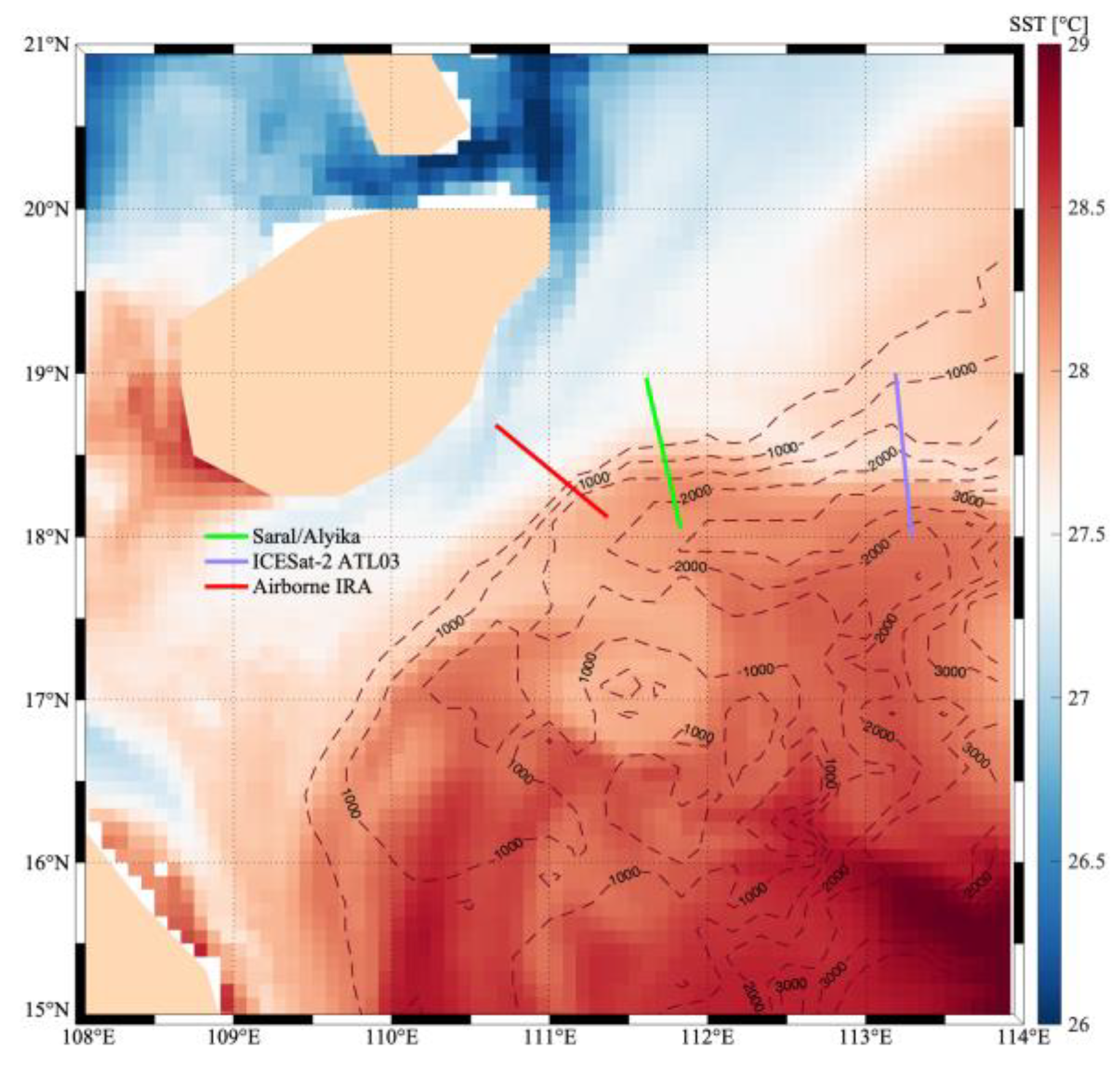
2.1.2. Study Site and Data Processing

The airborne IRA experiment was conducted over the South China Sea, particularly in the southeastern region of Hainan Province. This region is distinguished by a pronounced influence from interactions with the sea floor, tidal currents, and wind-driven phenomena. These factors collectively contribute to an amplification of submesoscale dynamics, making the region suitable for the experiment. The ground tracks of ICESat-2 ATL03 and SARAL/AltiKa pass through the vicinity. A Cessna-208B aircraft was used to carry the instruments of the onboard interferometric imaging altimeter system, along with the onboard Global Navigation Satellite System (GNSS) and inertial navigation devices. The track of airborne IRA, ICESat-2 ATL03, and SARAL/AltiKa is shown in Figure 1.
The processes of airborne IRA data include SAR imaging, primary and auxiliary image registration, interference processing, phase filtering, multi-look processing, and height inversion. We refer the reader to Yang et al. [17] and Sun et al. [14] for more details on the IRA instruments and processing. Outlier spike values were removed first. Height errors due to uncertainty in platform height and baseline inclination have their own spatial–temporal characteristics. These types of errors were extracted and reduced using Empirical Orthogonal Function (EOF) analysis. The SSHA was computed by applying tidal corrections and removing the mean sea surface (MSS) provided by the Collecte Localisation Satellites (CLS) group.

2.2. ICESat-2 ATL03

The ICESat-2 data used in this study are the SSHA data measured in November 2021. The Ice, Cloud, and Land Elevation Satellite-2 (ICESat-2) was launched in September 2018. The targets of the ICESat-2 satellite include forests, oceans, polar regions, as well as clouds and aerosols [20]. ATL03 is a data product from NASA’s ICESat-2 mission, which provides information about the Earth’s surface, including ocean waves. Yu et al. [19] used ICESat-2’s laser altimetry SSHA measurements (resolution: 15 m) and analyzed the SSHA wavenumber spectrum in the 500 km to 15 m range of the tropical Pacific Ocean. It carries a completely new laser photon-counting system, an advanced topographic laser altimeter system (ATLAS) [21]. Each ATLAS information product selected for unleashing begins with an associate “ATL” prefix, and details on all of the ICESat-2 products are available in their respective theoretical basis documents, which can be obtained from the National Snow & Ice Data Center. The basic input for determining wave characteristics on the ocean surface are derived from ATL03, which contains the individual geolocated photon information [22].

2.3. SARAL/AltiKa

The SARAL (Satellite with ARgos and ALtika) program is a collaborative initiative between the Indian Space Research Organisation (ISRO) and the French National Centre for Space Studies (CNES) [23]. It is primarily focused on ocean observations [23]. In the realm of oceans, SARAL/AltiKa enhances resolution and refines the accuracy of sea surface height signals, particularly in mesoscale observations [24,25,26]. These data represent near-real-time (NRT) SSHA, typically available within 7–9 h of measurement. Notably, these NRT data differ from the Operational Geophysical Data Record (OGDR) produced by the project, as SARAL’s orbit has been refined by adjusting SSHA differences with those from the OSTM/Jason-2 GPS-OGDR-SSHA product at inter-satellite crossover locations [23]. This adjustment enhances the accuracy of SARAL’s NRT orbit altitude to 1.5 cm (Root Mean Square), leveraging the 1 cm (radial Root Mean Square) accuracy of the GPS-based orbit used for the OSTM/Jason-2 GPS-OGDR-SSHA product [23].

2.4. MFWAM Wave Data

The MFWAM (Météo-France Wave Model) weather model is the world’s main weather forecast model for global ocean sea surface waves. It utilizes the ECWAM-IFS-38R2 computing code with a dissipation term developed by Ardhuin et al. [27]. The mean bathymetry of the model is generated using 2 min gridded global topography data from ETOPO2/NOAA, with the native model grid becoming irregular and decreasing in distance in the latitudinal direction closer to the poles. The distance in the latitudinal direction at the equator is fixed with a grid size of 1/10°. The operational model, MFWAM, is driven by 6-hourly analyses and 3-hourly forecasted winds from the IFS-ECMWF atmospheric system. The wave spectrum is discretized into 24 directions and 30 frequencies ranging from 0.035 Hz to 0.58 Hz. Additionally, the MFWAM model assimilates altimeter data with a time step of 6 h.

2.5. Methods

2.5.1. Wavenumber Spectrum Analysis

The wavenumber spectrum is a fundamental tool used in the analysis of spatial variations in physical quantities [28]. Wavenumber represents the number of wavelengths per unit distance. The wavenumber spectrum is obtained by performing a Fourier transform on a given spatial function or dataset [28,29]. The wavenumber spectrum provides information on the energy distribution across different spatial scales [29]. The shape and characteristics of the spectrum can reveal important information about the underlying physical processes [29].

2.5.2. Wave Parameter Retrieval

The IRA can provide 2D information on the Wave-Sea Surface Elevation (WSSE). The WSSE is the result of interactions of a large number of different waves and has a complicated pattern normally known as wind-generated gravity waves including wind waves and swell [30]. By analyzing the 2D WSSE, dominant wave direction can be extracted. The quality of the derived dominant wave direction can serve as a gauge for how well the IRA data perform. The retrieval method assumes that the dominant wave direction in a domain with 2D WSSE is the direction with the maximum number of gradients. The algorithm retrieves the dominant wave direction by analyzing the gradient distribution of the 2D WSSE. The dominant wavelength can be obtained by analyzing the variance-preserving wavenumber spectrum along the dominant wave direction. For a more comprehensive explanation, refer to the work of Jiang et al. [10].
SWH is a statistical average of the vertical movement of the WSSE and can be calculated from measured WSSE, using Equation (1) [31,32].
SWH = 4×〈τ21/2
where τ is the WSSE and 〈τ21/2 is the standard deviation of WSSE.

3. Results and Analyses

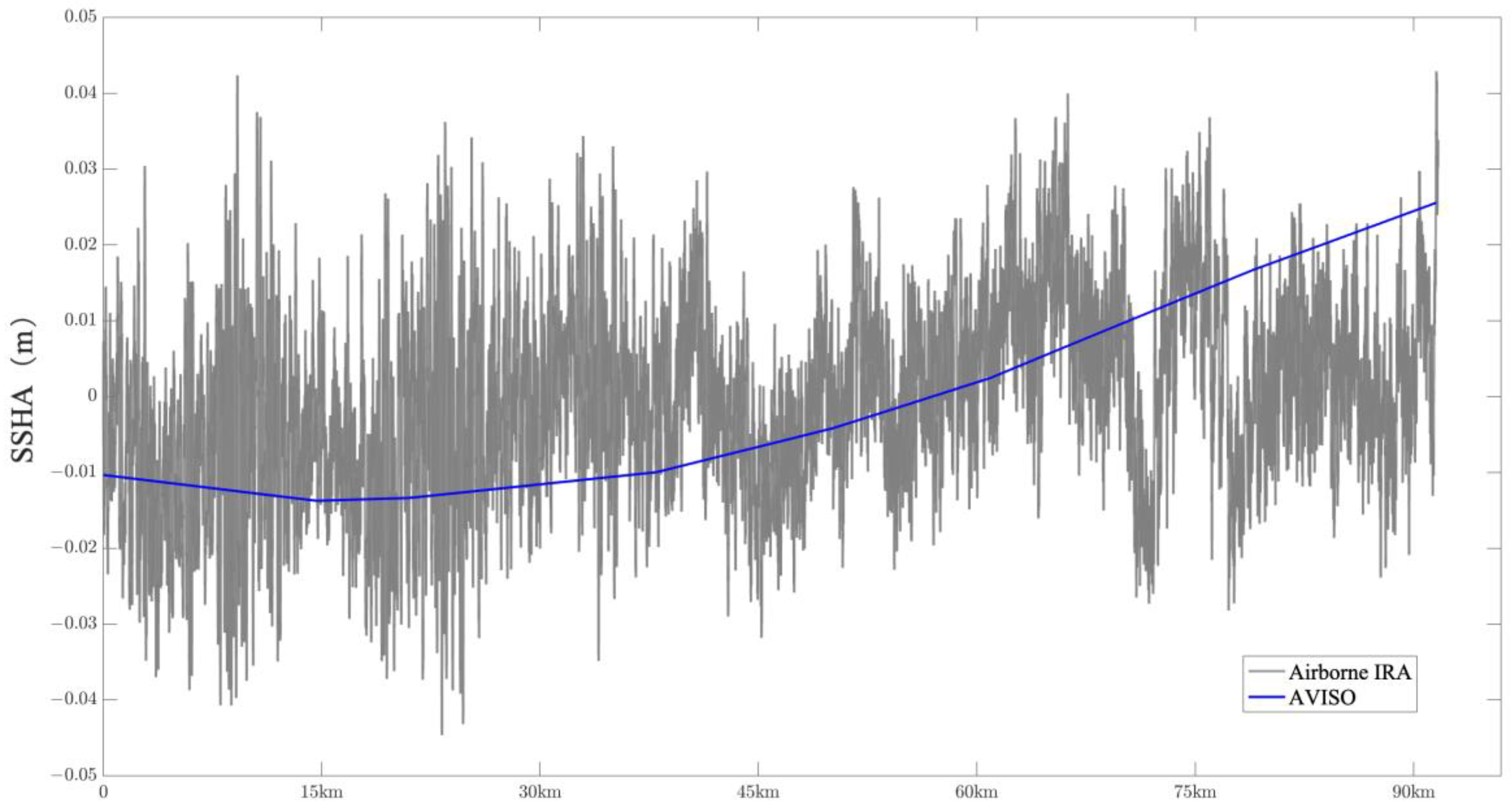
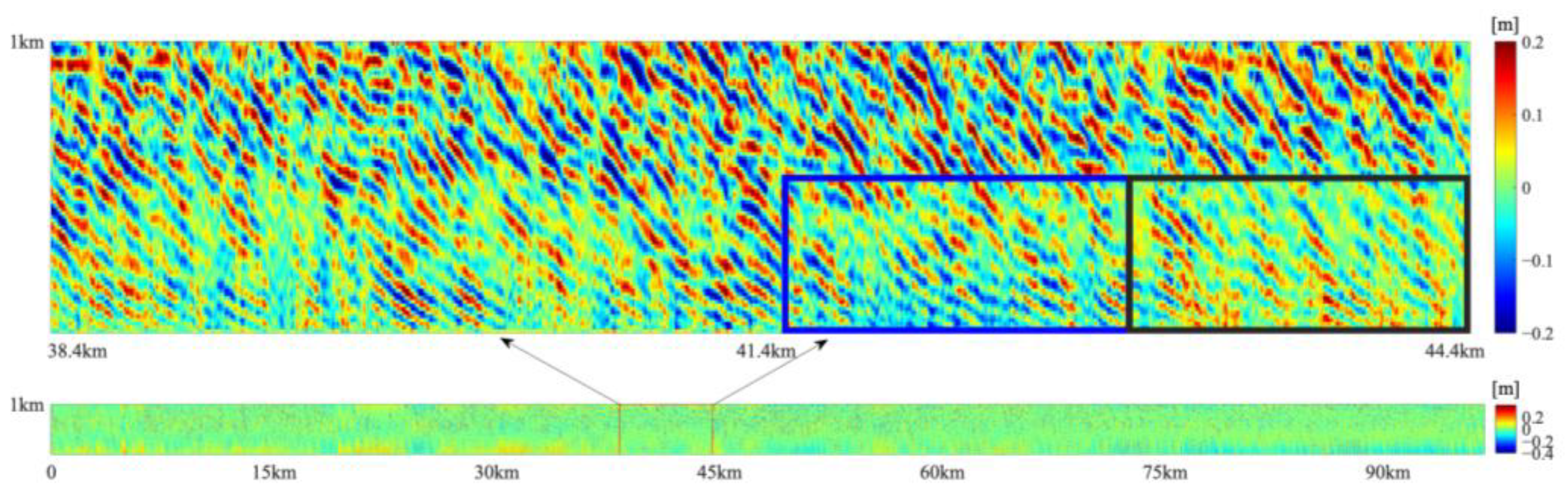
3.1. Sea Surface Height Anomaly

Figure 2 presents the along-track SSHA measured by the IRA, averaged across-track, in comparison with the SSHA from the gridded SSHA from AVISO on the same day, interpolated to the IRA track. It shows that the SSHA captured by the IRA has much more variability at shorter scales and that the short-scale variability is energetic over the entire submesoscale range. The energetic submesoscale processes in this region can be attributed to the interaction of vigorous ocean currents, winds, distinctive bathymetry, and pronounced temperature and salinity gradients [33]. At scales larger than 30 km, the IRA SSHA exhibits a rising trend along the track with a relatively steeper slope at a distance around 50 km, which is consistent with the trend of AVISO SSHA.
The AVISO SSHA exhibits significantly higher levels of smoothness in comparison to the IRA SSHA, mostly because of substantial data processing. This smoothness stems from spatial and temporal averaging, which diminishes short-term and small-scale fluctuations. Additionally, data interpolation fills gaps, inherently contributing to the dataset’s smoothness. The use of filtering techniques, such as low-pass filters, further removes noise and unwanted signals. These steps collectively enhance the smoothness of the AVISO SSHA, making it distinct in its clarity and consistency compared to the IRA SSHA.
The airborne IRA is capable of measuring 2D SSHA. Figure 3 shows the 2D SSHA from the IRA. The IRA shows a good ability to capture small-scale SSHA. In the enlarged image, waves featuring wavelengths between 50 and 150 m stand out as the most dominant feature. The submesoscale processes can occur on approximate scales of 0.1–10 km, with SSHA magnitudes typically smaller than ocean waves [2]. The superposition of waves with submesoscale SSHA complicates the identification of submesoscale SSHA. Nevertheless, it remains evident that the waves are superimposed on a background characterized by undulating heights. These fluctuations in the background are likely attributable to SSHA induced by submesoscale processes, as illustrated in the highlighted boxes in the enlarged image. The difference between the averaged SSHA in the two highlighted boxes in the enlarged image is about 3 cm. These fluctuations in the background are likely attributable to SSHA induced by submesoscale processes. Nevertheless, observing the smaller-scale part of the submesoscale SSHA remains challenging, due to the large SSHA of the wave motions, and the definition of the submesoscale SSHA remains elusive.

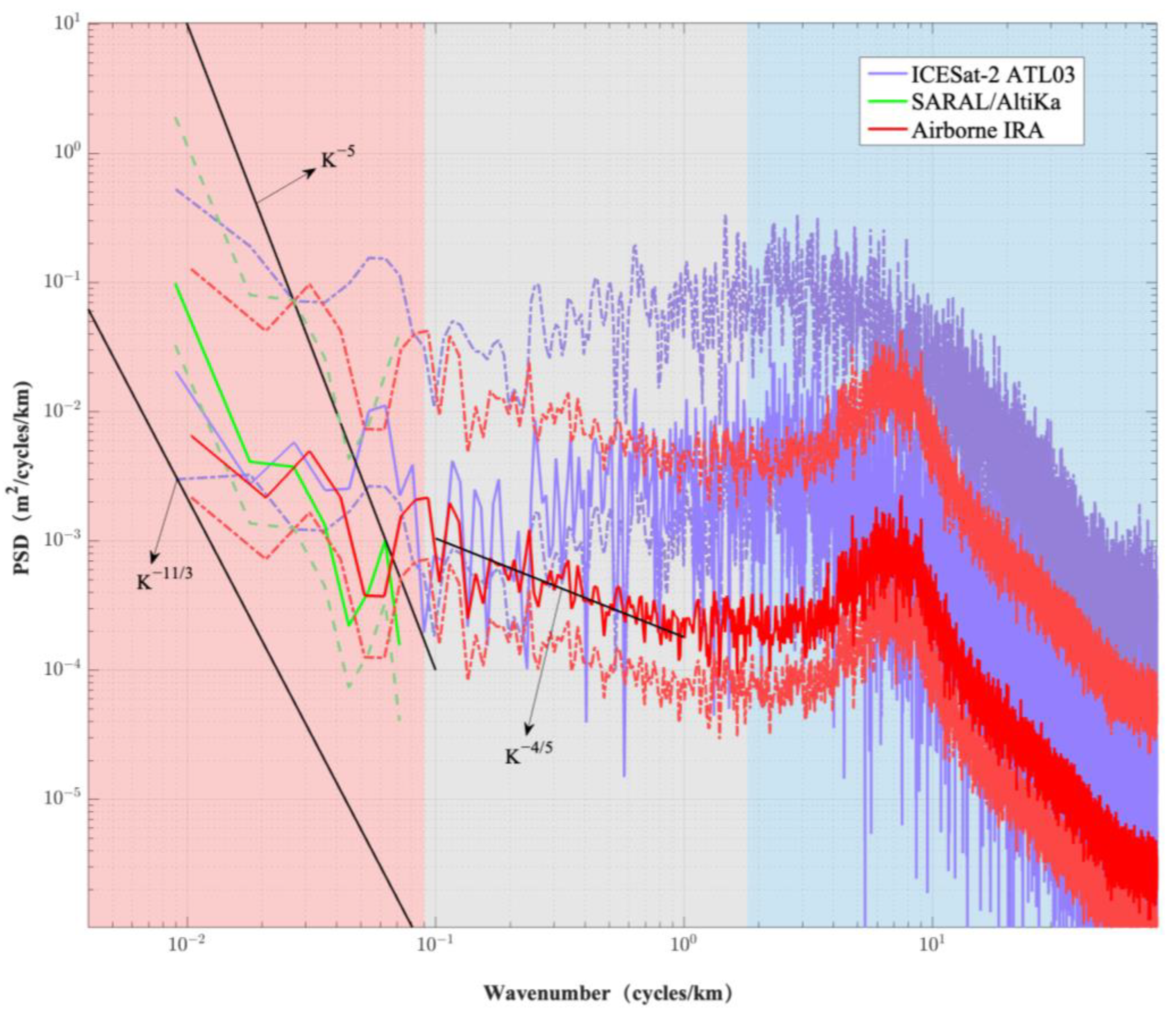
3.2. Wavenumber Spectrum

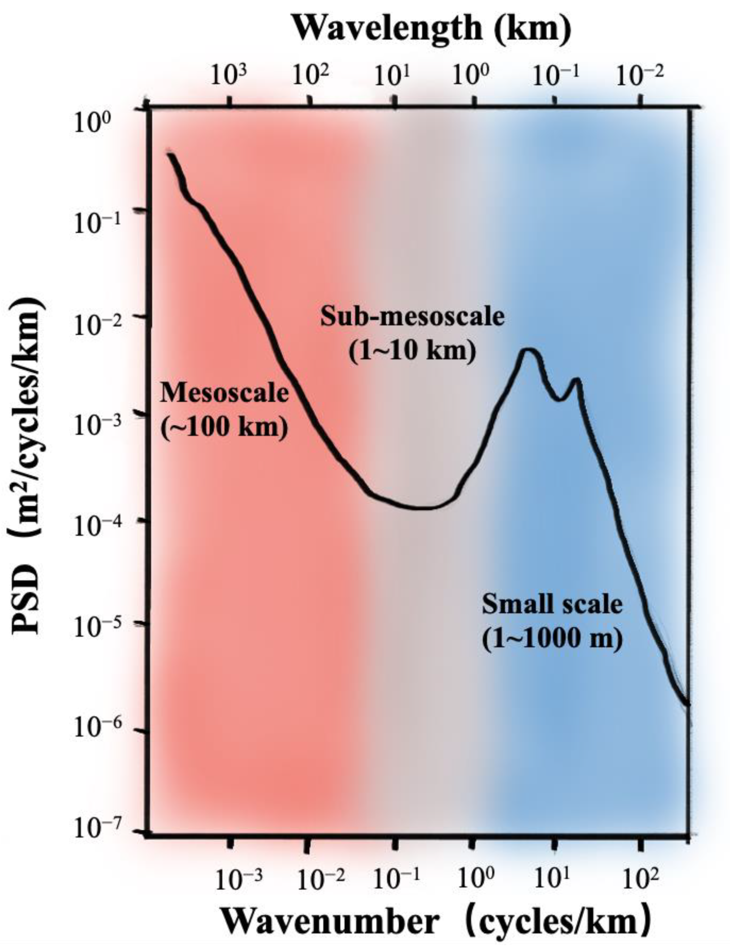
3.2.1. Expected Shape of Wavenumber Spectrum

Energy balance in ocean dynamics holds the key to predicting the state of ocean circulation and its evolution. The oceanic wavenumber spectrum can help diagnose energy balance and cascades. Mesoscale (tens to hundreds of kilometers) eddies are dominant motions in the upper ocean. Based on assumptions of geostrophic balance and conservations of energy and potential vorticity, the theories of quasigeostrophic turbulence predict a wavenumber (k) spectrum with spectral slopes spanning from k−5 to k−11/3 for wavenumbers in the mesoscale to submesoscale range (red zone in Figure 4) [34,35]. The shape of the theoretical mesoscale spectrum has been confirmed through satellite altimeter observations [15,36]. However, the instrumental noise of conventional altimeters has a significant effect on the slope of the wavenumber spectrum for sea surface heights on scales below 50 km, bringing them close to the white noise floor [16].
The spatial scale and energy level of the submesoscale SSHA, which ranges from about one to tens of kilometers (gray zone in Figure 4), is typically more than an order of magnitude smaller than that of the mesoscale, creating a gap in the wavenumber spectrum between the mesoscale and the scale of surface gravity waves, with PSD levels typically less than 10−3 m2/cycle/km [4,37]. The slope of the wavenumber spectrum for submesoscale SSHA can vary depending on the specific dynamics and environmental conditions, but with a downward trend similar to that of the mesoscale. Submesoscale SSHAs are driven by frontogenesis, instability, strain, topographic interactions, etc. However, submesoscale SSHAs can often be masked by internal waves, resulting in a flatter spectral slope. The lack of observations in this range makes it difficult to understand the role of each process. The instrumental noise of satellite altimetry (with zero spectral slope) is generally higher than the energy level of submesoscale SSHA in the smaller-scale part. Therefore, the lower the energy levels and the steeper the slope observed by satellites at submesoscales, the greater the likelihood of observing oceanic submesoscale processes.
At scales ranging from hundreds of meters to a few meters, the wavenumber spectrum of the sea surface elevation is dominated by surface gravity waves (blue zone in Figure 4). The wavenumber spectrum of ocean gravity waves typically exhibits a distinct shape characterized by a peak at a certain wavenumber. The peak of the spectrum corresponds to the dominant wavenumber, which represents the most energetic or prevalent wave scale in the ocean at a particular location and time. As the wavenumber increases beyond the peak, the energy content of the waves decreases rapidly. This decrease in energy at higher wavenumbers represents the diminishing contribution of smaller-scale waves to the overall wave energy spectrum. The specific shape of the wave spectrum is influenced by various factors, including wind speed, water depth, and fetch (the distance over which the wind blows) [38].

3.2.2. Observed Wavenumber Spectra

In this study, we examine the wavenumber spectra of IRA, ICESat-2, and SARAL/AltiKa. The Welch method [39] was utilized for power spectral density estimation of the airborne IRA and SARAL/AltiKa, and all IRA along-track spectra were averaged. A three-point moving average was applied to the ICESat-2 ATL03 data to reduce noise before estimating the wavenumber spectrum.
Figure 5 compares the SSHA wavenumber spectra of the Interferometric Radar Altimeter (IRA), ICESat-2 ATL03, and SARAL/AltiKa. At wavelengths exceeding 30 km (rightmost part of the red zone), the IRA spectrum resembles those of SARAL/AltiKa and ICESat-2 ATL03 in both shape and PSD level. All three spectra exhibit a “red” character, with similar energy levels below 0.03 cycles km−1 and a spectral slope close to the typical mesoscale turbulence range between k−5 and k−11/3, consistent with the spectra from satellite observations. This indicates that the IRA has a reasonable energy distribution at spatial scales near the mesoscale, consistent with the result in Figure 4.
The relatively shallower spectral slopes observed in IRA can be attributed to two factors. Firstly, the SSH wavenumber slope exhibits geographical variations [15], and the IRA track is positioned closer to the island compared to the satellite tracks (Figure 1). Secondly, the shorter length of the IRA track (less than 100 km) introduces larger uncertainties in the spectrum at scales exceeding 30 km. The confidence levels for various SSH spectra are depicted in Figure 5.
However, significant differences emerge at submesoscales (wavelengths below 30 km). While the SARAL/AltiKa and ICESat-2 ATL03 spectra become significantly flatter, the IRA spectrum maintains a clear negative slope down to approximately 1 km, consistent with theoretical prediction. This suggests that noise contamination affects SARAL/AltiKa and ICESat-2 ATL03, hindering their ability to resolve submesoscale SSHA. Furthermore, the IRA’s resolved PSD level in the 1–10 km submesoscale range is roughly ten times lower than that of ICESat-2 ATL03, demonstrating the airborne IRA’s superior capability to resolve lower-energy SSHA variations. The minimum PSD level of the IRA fell in the range of 10−4–10−3 m2/cycle/km. This is significantly lower, by more than an order of magnitude, compared to the measurements of ICESat-2. This discrepancy results in a spectral gap that aligns with theoretical predictions. The precise slope of the wave number spectrum at the submesoscale remains a subject of active investigation. While submesoscale processes such as mixed-layer instabilities and frontogenesis can be drivers of SSHA variations at this scale, there are far more factors that can have an impact on SSHA [2]. Internal waves, characterized by their ability to propagate long distances while affecting the vertical structure of the water column, and horizontally diverging currents, which contribute to the redistribution of water masses, play an important role in shaping SSHA patterns [2,40]. In addition, external factors such as the wind setup effect, geoid uncertainty, and thermal expansion due to temperature changes also contribute to the complexity of SSHA dynamics [2,41,42]. The cumulative effect of these diverse processes may underlie the observed negative slope in the IRA SSHA spectrum at this scale. Investigating the effects of these multiple factors provides a more comprehensive understanding of the mechanisms driving SSHA variability [18].
The observed IRA spectrum exhibits a k−1.3 slope in the 1–30 km range, significantly shallower than the k−11/3 slope expected for mesoscale eddies [2] and the k−2 slope advocated by Qiu et al. [43] and Torres et al. [44]. This deviation may stem from two factors: (1) The SSH wavenumber slope can vary significantly with time [45]. Similar variability could affect the 1–30 km range, leading to deviations from the expected slopes. The IRA track is near shore and crosses SST fronts parallel to the coastline (Figure 1). The topography of the coastal shelf can significantly affect the SSHA in several ways, including current steering and deflection, friction, coastal trapped waves, and upwelling and downwelling, contributing to the presence of more short-scale SSH variability in the IRA observations [46,47,48]. (2) Uncertainty in submesoscale SSH spectrum: McWilliams [30] focuses on velocity wavenumber slopes, lacking explicit discussion of SSH spectra near the submesoscale range. While their analysis suggests a k−5/3 velocity slope for velocity wavenumbers in the mesoscale-to-submesoscale transition, this does not directly translate to a k−11/3 SSH wavenumber slope within the 1–30 km range. This discrepancy arises because the expected k−2 slope difference under geostrophic balance does not hold strictly near the submesoscales, where geostrophic balance weakens. This can lead to complexities in the SSH wavenumber slope within the submesoscale range.
In the scale range of gravity wave (blue zone), the shape and energy level of ICESat-2 and IRA SSHA spectra are comparable. Both have a peak at a particular wavenumber corresponding to a dominant wavenumber. As the wavenumber decreases from the peak, the wave energy decreases, resulting in a rapid decline in the spectrum. This decline is steeper on the high-wavenumber side of the peak compared to the low-wavenumber side, consistent with the theoretical prediction of JONSWAP wave spectrum [49]. In deep water, the decline in the wavenumber spectrum is generally more gradual and less steep compared to shallow water. The spectrum may exhibit a more uniform distribution of wave energy across a wider range of wavenumbers. This prediction is further supported by the analysis of wavenumber spectra from ICESat-2 ATL03 and IRA SSHA data. It is noteworthy that the ICESat-2 ATL03 track covers a region with greater water depth compared to the airborne IRA.

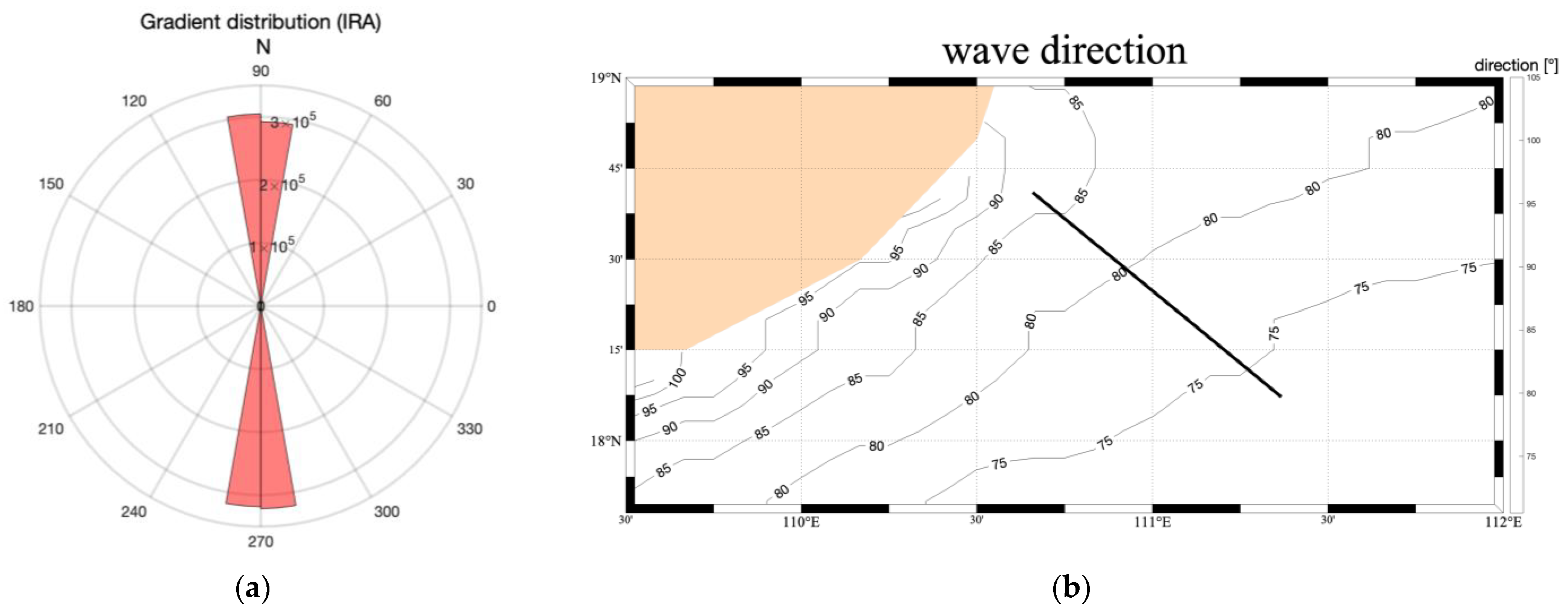
3.2.3. Wave Parameter Analysis

To further assess the effectiveness of airborne IRA measurements for wave monitoring, we compared wave parameters (dominant direction, wavelength, and SWH) extracted from 2D airborne IRA data with those from the MFWAM wave model. We employed the retrieval method proposed by Jiang et al. [10] for extracting these wave parameters from the IRA data. While Jiang et al. [10] analyzed a 1 km segment in the coastal region, we averaged these retrieved parameters over a 90 km path for a more robust estimate. And because the wavelengths of gravity waves generated by wind are roughly between 1.5 and 900 m [30], we filtered the data for wavelengths above 250 m. We identified the dominant wave direction as approximately 90 degrees by analyzing the gradient distribution in Figure 6a. Subsequently, the averaged SWH derived from the IRA WSSE is 0.82 m.
Figure 6b presents the wave direction as per the MFWAM wave data, which also indicates a direction close to 90 degrees in this region. Such a difference is to be expected given the spatial and temporal inconsistencies inherent in data collection and the uncertainty in the boundary conditions of the model data. Furthermore, the SWH of MFWAM in this region is 0.73 m, closely matching those obtained from the IRA measurements.

4. Discussion

Conventional nadir-looking radar altimeters have a footprint of the order of 2–10 km. Even with thousands of pulses averaging over 1 s, the noise level in SSHA measurements still obscures ocean SSHA signals at wavelengths shorter than 100 km. This limitation is evident in the noise floor observed in the along-track SSHA wavenumber spectrum of satellite radar altimeters, as highlighted by Fu and Ferrari [50]. After mitigating the effects of instrument noise, Xu and Fu [16] showed that the energy level below 100 km continues to decrease with wavenumber toward the submesoscale. Two distinct features are expected in the submesoscale SSHA wavenumber spectrum: a negative slope and the minimum energy level. These features are indeed present in the IRA SSHA wavenumber spectrum. Furthermore, the IRA’s minimum PSD level fell in the range of 10−4 to 10−3 m2/cycle/km, forming a spectral gap between meso-to-submesoscale motions and small-scale surface waves. This gap is consistent with the theoretical expectation, indicating the rationality of the wavenumber spectrum. It is unlikely that the error-dominated SSHA wavenumber spectrum has these features.
Although conventional satellite radar altimetry has changed our understanding of many oceanographic phenomena at large and mesoscales, the temporal and spatial resolution of the present constellation is insufficient to observe the two-dimensional structure of SSHA variability at scales shorter than 150 km [51]. The SWOT mission has changed this paradigm by mapping the SSHA via two parallel 50 km wide swaths, capable of resolving processes with wavelengths as small as ~15 km. However, it is still challenging for satellite interferometry to resolve the SSHA variability in the submesosale range of 1–10 km. Furthermore, traditional altimeters are restricted to one-dimensional measurements, hindering their ability to capture the nuances of submesoscale variations. In contrast, the IRA facilitates two-dimensional observations and has the potential to broaden the scope of its swath measurements. For the first time, we illustrate that an IRA-type altimeter possesses the potential to identify two-dimensional SSHA variability within the submesoscale domain (less than 10 km), bridging a gap in observational capabilities. We anticipate that our study will inspire a renewed appreciation for the potential of airborne IRA in detecting two-dimensional small submesoscale SSHA. These processes are vital for understanding ocean dynamics, marine ecosystems, and their role in the Earth’s climate system.

Author Contributions

Y.X. conceived the main ideas and methods for this paper. J.H. handled the data processing and analysis. Y.X. and J.H. collaborated to complete the initial draft of the manuscript. H.S. and W.K. contributed by providing IRA data for the research. Q.J. and L.Y. contributed a portion of the code used in this research. Y.L. contributed the data processing. All authors have read and agreed to the published version of the manuscript.

Funding

This research was supported by Laoshan Laboratory science and technology innovation projects (No. LSKJ202201406-2), NSFC-Shandong Joint Fund Key Project (No. U22A20587), and Innovative Practice Training Program of University of the National Academy of Sciences (No. Y5KY09101L).

Data Availability Statement

The AVISO data hosted by the PO.DAAC are openly shared, without restriction, in accordance with NASA’s Earth Science program Data and Information Policy (at https://doi.org/10.5067/SLREF-CDRV3, accessed on 20 July 2023). ICESat-2 data are available through the National Snow and Ice Data Center (NSIDC). The sea surface height product is found online (at https://nsidc.org/data/ATL03, accessed on 19 July 2022). The MFWAM model was conducted using E.U. Copernicus Marine Service Information; DOI: https://doi.org/10.48670/moi-00022, accessed on 6 April 2023. The SARAL/AltiKa data hosted by the PO.DAAC are openly shared, without restriction, in accordance with NASA’s Earth Science program Data and Information Policy (at https://doi.org/10.5067/AKASA-XOGD1, accessed on 20 September 2023).The SST data was conducted using E.U. Copernicus Marine Service Information; DOI https://doi.org/10.48670/moi-00016, accessed on 6 February 2024.

Acknowledgments

The authors would like to thank the technical crew of the Guanlan ocean science mission for the interferometric radar altimeter (IRA) data sampling in the South China Sea experiment.

Conflicts of Interest

The authors declare no conflicts of interest.

References

  1. Shutler, J.D.; Quartly, G.D.; Donlon, C.J.; Sathyendranath, S.; Platt, T.; Chapron, B.; Johannessen, J.A.; Girard-Ardhuin, F.; Nightingale, P.D.; Woolf, D.K.; et al. Progress in Satellite Remote Sensing for Studying Physical Processes at the Ocean Surface and Its Borders with the Atmosphere and Sea Ice. Prog. Phys. Geogr. Earth Environ. 2016, 40, 215–246. [Google Scholar] [CrossRef]
  2. McWilliams, J.C. Submesoscale Currents in the Ocean. Proc. R. Soc. A 2016, 472, 20160117. [Google Scholar] [CrossRef] [PubMed]
  3. Srinivasan, M.; Tsontos, V. Satellite Altimetry for Ocean and Coastal Applications: A Review. Remote Sens. 2023, 15, 3939. [Google Scholar] [CrossRef]
  4. Villas Bôas, A.B.; Lenain, L.; Cornuelle, B.D.; Gille, S.T.; Mazloff, M.R. A Broadband View of the Sea Surface Height Wavenumber Spectrum. Geophys. Res. Lett. 2022, 49, e2021GL096699. [Google Scholar] [CrossRef]
  5. Wang, J.; Fu, L.-L.; Torres, H.S.; Chen, S.; Qiu, B.; Menemenlis, D. On the Spatial Scales to Be Resolved by the Surface Water and Ocean Topography Ka-Band Radar Interferometer. J. Atmos. Ocean. Technol. 2019, 36, 87–99. [Google Scholar] [CrossRef]
  6. Fu, L.-L.; Pavelsky, T.; Cretaux, J.-F.; Morrow, R.; Farrar, J.T.; Vaze, P.; Sengenes, P.; Vinogradova-Shiffer, N.; Sylvestre-Baron, A.; Picot, N.; et al. The Surface Water and Ocean Topography Mission: A Breakthrough in Radar Remote Sensing of the Ocean and Land Surface Water. Geophys. Res. Lett. 2024, 51, e2023GL107652. [Google Scholar] [CrossRef]
  7. Tuozzolo, S.; Lind, G.; Overstreet, B.; Mangano, J.; Fonstad, M.; Hagemann, M.; Frasson, R.P.M.; Larnier, K.; Garambois, P.-A.; Monnier, J.; et al. Estimating River Discharge with Swath Altimetry: A Proof of Concept Using AirSWOT Observations. Geophys. Res. Lett. 2019, 46, 1459–1466. [Google Scholar] [CrossRef]
  8. Altenau, E.H.; Pavelsky, T.M.; Moller, D.; Lion, C.; Pitcher, L.H.; Allen, G.H.; Bates, P.D.; Calmant, S.; Durand, M.; Smith, L.C. AirSWOT Measurements of River Water Surface Elevation and Slope: Tanana River, AK. Geophys. Res. Lett. 2017, 44, 181–189. [Google Scholar] [CrossRef]
  9. Wang, Y.; Bai, Y.; Zhang, Y.; Sun, D.; Chen, G.; Yu, F.; Zhao, C.; Sun, H.; Wei, L.; Yang, L.; et al. Impact of Ocean Waves on the Decorrelation of Interferometric Radar Altimeter Image. IEEE Geosci. Remote Sens. Lett. 2022, 19, 1–5. [Google Scholar] [CrossRef]
  10. Jiang, Q.; Xu, Y.; Sun, H.; Wei, L.; Yang, L.; Zheng, Q.; Jiang, H.; Zhang, X.; Qian, C. Wind-Generated Gravity Waves Retrieval from High-Resolution 2-D Maps of Sea Surface Elevation by Airborne Interferometric Altimeter. IEEE Geosci. Remote Sens. Lett. 2021, 19, 1–5. [Google Scholar] [CrossRef]
  11. Sun, D.; Wang, Y.; Zhang, Y.; Sun, H.; Yang, L.; Yu, F. Wind Wave and Wind Speed Inversion Based on Azimuth Cutoff of Airborne IRA Images. IEEE Trans. Geosci. Remote Sens. 2024, 62, 1–14. [Google Scholar] [CrossRef]
  12. Sun, D.; Zhang, Y.; Wang, Y.; Chen, G.; Sun, H.; Yang, L.; Bai, Y.; Yu, F.; Zhao, C. Ocean Wave Inversion Based on Airborne IRA Images. IEEE Trans. Geosci. Remote Sens. 2022, 60, 1–13. [Google Scholar] [CrossRef]
  13. Qiu, Z.; Ma, C.; Wang, Y.; Yu, F.; Sun, H.; Zhao, S.; Yang, L.; Tang, J.; Chen, G. Improving Sea Surface Height Reconstruction by Simultaneous Ku- and Ka-Band Near-Nadir Single-Pass Interferometric SAR Altimeter. IEEE Trans. Geosci. Remote Sens. 2023, 61, 1–14. [Google Scholar] [CrossRef]
  14. Sun, D.; Wang, Y.; Xu, Z.; Zhang, Y.; Zhang, Y.; Meng, J.; Sun, H.; Yang, L. Ocean Wave Inversion Based on Hybrid Along- and Cross-Track Interferometry. Remote Sens. 2022, 14, 2793. [Google Scholar] [CrossRef]
  15. Xu, Y.; Fu, L.-L. Global Variability of the Wavenumber Spectrum of Oceanic Mesoscale Turbulence. J. Phys. Oceanogr. 2011, 41, 802–809. [Google Scholar] [CrossRef]
  16. Xu, Y.; Fu, L.-L. The Effects of Altimeter Instrument Noise on the Estimation of the Wavenumber Spectrum of Sea Surface Height. J. Phys. Oceanogr. 2012, 42, 2229–2233. [Google Scholar] [CrossRef]
  17. Yang, L.; Xu, Y.; Zhou, X.; Zhu, L.; Jiang, Q.; Sun, H.; Chen, G.; Wang, P.; Mertikas, S.P.; Fu, Y. Calibration of an Airborne Interferometric Radar Altimeter over the Qingdao Coast Sea, China. Remote Sens. 2020, 12, 1651. [Google Scholar] [CrossRef]
  18. Rocha, C.B.; Chereskin, T.K.; Gille, S.T.; Menemenlis, D. Mesoscale to Submesoscale Wavenumber Spectra in Drake Passage. J. Phys. Oceanogr. 2016, 46, 601–620. [Google Scholar] [CrossRef]
  19. Yu, Y.; Sandwell, D.T.; Gille, S.T.; Villas Bôas, A.B. Assessment of ICESat-2 for the Recovery of Ocean Topography. Geophys. J. Int. 2021, 226, 456–467. [Google Scholar] [CrossRef]
  20. Horvat, C.; Blanchard-Wrigglesworth, E.; Petty, A. Observing Waves in Sea Ice with ICESat-2. Geophys. Res. Lett. 2020, 47, e2020GL087629. [Google Scholar] [CrossRef]
  21. Zhao, Y.; Wu, B.; Shu, S.; Yang, L.; Wu, J.; Yu, B. Evaluation of ICESat-2 ATL03/08 Surface Heights in Urban Environments Using Airborne LiDAR Point Cloud Data. IEEE Geosci. Remote Sens. Lett. 2021, 19, 1–5. [Google Scholar] [CrossRef]
  22. Klotz, B.W.; Neuenschwander, A.; Magruder, L.A. High-Resolution Ocean Wave and Wind Characteristics Determined by the ICESat-2 Land Surface Algorithm. Geophys. Res. Lett. 2020, 47, e2019GL085907. [Google Scholar] [CrossRef]
  23. Verron, J.; Sengenes, P.; Lambin, J.; Noubel, J.; Steunou, N.; Guillot, A.; Picot, N.; Coutin-Faye, S.; Sharma, R.; Gairola, R.M.; et al. The SARAL/AltiKa Altimetry Satellite Mission. Mar. Geod. 2015, 38, 2–21. [Google Scholar] [CrossRef]
  24. Verron, J.; Bonnefond, P.; Andersen, O.; Ardhuin, F.; Bergé-Nguyen, M.; Bhowmick, S.; Blumstein, D.; Boy, F.; Brodeau, L.; Crétaux, J.-F. The SARAL/AltiKa Mission: A Step Forward to the Future of Altimetry. Adv. Space Res. 2021, 68, 808–828. [Google Scholar] [CrossRef]
  25. Verron, J.; Bonnefond, P.; Aouf, L.; Birol, F.; Bhowmick, S.A.; Calmant, S.; Conchy, T.; Crétaux, J.-F.; Dibarboure, G.; Dubey, A.K. The Benefits of the Ka-Band as Evidenced from the SARAL/AltiKa Altimetric Mission: Scientific Applications. Remote Sens. 2018, 10, 163. [Google Scholar] [CrossRef]
  26. Dibarboure, G.; Lamy, A.; Pujol, M.-I.; Jettou, G. The Drifting Phase of SARAL: Securing Stable Ocean Mesoscale Sampling with an Unmaintained Decaying Altitude. Remote Sens. 2018, 10, 1051. [Google Scholar] [CrossRef]
  27. Collard, F. Semi-Empirical Dissipation Source Functions for Wind-Wave Models: Part I, Definition, Calibration and Validation at Global Scales. J. Phys. Oceanogr. 2010, 40, 1917–1941. [Google Scholar]
  28. Capon, J. High-Resolution Frequency-Wavenumber Spectrum Analysis. Proc. IEEE 1969, 57, 1408–1418. [Google Scholar] [CrossRef]
  29. Storer, B.A.; Buzzicotti, M.; Khatri, H.; Griffies, S.M.; Aluie, H. Global Energy Spectrum of the General Oceanic Circulation. Nat. Commun. 2022, 13, 5314. [Google Scholar] [CrossRef]
  30. Toffoli, A.; Bitner-Gregersen, E.M. Types of Ocean Surface Waves, Wave Classification. In Encyclopedia of Maritime and Offshore Engineering; Carlton, J., Jukes, P., Choo, Y.S., Eds.; Wiley: Hoboken, NJ, USA, 2017; pp. 1–8. ISBN 978-1-118-47635-2. [Google Scholar]
  31. Hoffman, D.; Karst, O.J. The Theory of the Rayleigh Distribution and Some of Its Applications. J. Ship Res. 1975, 19, 172–191. [Google Scholar] [CrossRef]
  32. Stewart, R.H. Introduction to Physical Oceanography; Texas A & M University: College Station, TX, USA, 2008. [Google Scholar]
  33. Zheng, Q.; Xie, L.; Xiong, X.; Hu, X.; Chen, L. Progress in Research of Submesoscale Processes in the South China Sea. Acta Oceanol. Sin. 2020, 39, 1–13. [Google Scholar] [CrossRef]
  34. Charney, J.G. Geostrophic Turbulence. J. Atmos. Sci. 1971, 28, 1087–1095. [Google Scholar] [CrossRef]
  35. Blumen, W. Uniform Potential Vorticity Flow: Part I. Theory of Wave Interactions and Two-Dimensional Turbulence. J. Atmos. Sci. 1978, 35, 774–783. [Google Scholar] [CrossRef]
  36. Stammer, D. Global Characteristics of Ocean Variability Estimated from Regional TOPEX/POSEIDON Altimeter Measurements. J. Phys. Oceanogr. 1997, 27, 1743–1769. [Google Scholar] [CrossRef]
  37. Taylor, J.R.; Thompson, A.F. Submesoscale Dynamics in the Upper Ocean. Annu. Rev. Fluid Mech. 2023, 55, 103–127. [Google Scholar] [CrossRef]
  38. Jing, Z.; Fox-Kemper, B.; Cao, H.; Zheng, R.; Du, Y. Submesoscale Fronts and Their Dynamical Processes Associated with Symmetric Instability in the Northwest Pacific Subtropical Ocean. J. Phys. Oceanogr. 2020, 51, 83–100. [Google Scholar] [CrossRef]
  39. Same, M.H.; Gandubert, G.; Gleeton, G.; Ivanov, P.; Landry, R., Jr. Simplified Welch Algorithm for Spectrum Monitoring. Appl. Sci. 2020, 11, 86. [Google Scholar] [CrossRef]
  40. Savage, A.C.; Arbic, B.K.; Alford, M.H.; Ansong, J.K.; Farrar, J.T.; Menemenlis, D.; O’Rourke, A.K.; Richman, J.G.; Shriver, J.F.; Voet, G.; et al. Spectral Decomposition of Internal Gravity Wave Sea Surface Height in Global Models. J. Geophys. Res. Ocean. 2017, 122, 7803–7821. [Google Scholar] [CrossRef]
  41. Zhang, Y.; Wallace, J.M.; Battisti, D.S. ENSO-like Interdecadal Variability: 1900–1993. J. Clim. 1997, 10, 1004–1020. [Google Scholar] [CrossRef]
  42. Casey, K.S.; Adamec, D. Sea Surface Temperature and Sea Surface Height Variability in the North Pacific Ocean from 1993 to 1999. J. Geophys. Res. 2002, 107, 14-1–14-12. [Google Scholar] [CrossRef]
  43. Qiu, B.; Chen, S.; Klein, P.; Wang, J.; Torres, H.; Fu, L.-L.; Menemenlis, D. Seasonality in Transition Scale from Balanced to Unbalanced Motions in the World Ocean. J. Phys. Oceanogr. 2018, 48, 591–605. [Google Scholar] [CrossRef]
  44. Torres, H.S.; Klein, P.; Menemenlis, D.; Qiu, B.; Su, Z.; Wang, J.; Chen, S.; Fu, L. Partitioning Ocean Motions into Balanced Motions and Internal Gravity Waves: A Modeling Study in Anticipation of Future Space Missions. JGR Ocean. 2018, 123, 8084–8105. [Google Scholar] [CrossRef]
  45. Hu, Q.; Huang, X.; Zhang, Z.; Zhang, X.; Xu, X.; Sun, H.; Zhou, C.; Zhao, W.; Tian, J. Cascade of Internal Wave Energy Catalyzed by Eddy-Topography Interactions in the Deep South China Sea. Geophys. Res. Lett. 2020, 47, e2019GL086510. [Google Scholar] [CrossRef]
  46. Woodworth, P.L.; Melet, A.; Marcos, M.; Ray, R.D.; Wöppelmann, G.; Sasaki, Y.N.; Cirano, M.; Hibbert, A.; Huthnance, J.M.; Monserrat, S.; et al. Forcing Factors Affecting Sea Level Changes at the Coast. Surv. Geophys. 2019, 40, 1351–1397. [Google Scholar] [CrossRef]
  47. Strub, P.T.; Combes, V.; Shillington, F.A.; Pizarro, O. Currents and Processes along the Eastern Boundaries. In International Geophysics; Elsevier: Amsterdam, The Netherlands, 2013; Volume 103, pp. 339–384. [Google Scholar]
  48. Ray, S.; Swain, D.; Ali, M.M.; Bourassa, M.A. Coastal Upwelling in the Western Bay of Bengal: Role of Local and Remote Windstress. Remote Sens. 2022, 14, 4703. [Google Scholar] [CrossRef]
  49. Hasselmann, K.; Barnett, T.P.; Bouws, E.; Carlson, H.; Cartwright, D.E.; Enke, K.; Ewing, J.A.; Gienapp, A.; Hasselmann, D.E.; Kruseman, P.; et al. Measurements of Wind-Wave Growth and Swell Decay during the Joint North Sea Wave Project (JONSWAP). Ergaenzungsheft Zur Dtsch. Hydrogr. Z. Reihe A 1973, 12, 1–95. [Google Scholar]
  50. Fu, L.; Ferrari, R. Observing Oceanic Submesoscale Processes from Space. EoS Trans. 2008, 89, 488. [Google Scholar] [CrossRef]
  51. Morrow, R.; Fu, L.-L.; Ardhuin, F.; Benkiran, M.; Chapron, B.; Cosme, E.; d’Ovidio, F.; Farrar, J.T.; Gille, S.T.; Lapeyre, G. Global Observations of Fine-Scale Ocean Surface Topography with the Surface Water and Ocean Topography (SWOT) Mission. Front. Mar. Sci. 2019, 6, 232. [Google Scholar] [CrossRef]
Figure 1. The track of airborne interferometric altimeters, ICESat-2 ATL03 and SARAL/AltiKa. The color on the map represents the sea surface temperature (SST) on 6 November 2021.
Remotesensing 16 01359 g001
Figure 2. Across-track-averaged SSHA for airborne IRA (gray); gridded SSHA from AVISO for 6 November 2021 interpolated to the IRA track coordinates (blue).
Remotesensing 16 01359 g002
Figure 3. 2D SSHA from the IRA measurements.
Remotesensing 16 01359 g003
Figure 4. Schematic SSH wavenumber spectra. The red, grey, and blue areas in the background are the three different spectral regions defined in this paper (adapted from Villas Bôas et al. [4], Figure 1).
Remotesensing 16 01359 g004
Figure 5. Wavenumber spectrum of IRA, ICESat-2 ATL03, and SARAL/AltiKa. In the background are three defined spectral regions. The shallow red, green, and purple dashed lines are 90% confidence intervals for IRA, SARAL/AltiKa, and ICESat-2 ATL03, respectively.
Remotesensing 16 01359 g005
Figure 6. (a) The gradient distribution in the wave direction of IRA; (b) wave direction from the MFWAM wave data.
Remotesensing 16 01359 g006
Table 1. Parameters of the airborne IRA.
ParameterKa Band
Radar frequency35.8 GHz
Baseline length0.34 m
Incidence angle1–15°
Range pixel spacing3 m
Along track pixel spacing3 m
Flight altitude3767 m
Flight speed70 m/s
Disclaimer/Publisher’s Note: The statements, opinions and data contained in all publications are solely those of the individual author(s) and contributor(s) and not of MDPI and/or the editor(s). MDPI and/or the editor(s) disclaim responsibility for any injury to people or property resulting from any ideas, methods, instructions or products referred to in the content.

