1. Introduction
Roughly one-quarter of the terrestrial area in the Northern Hemisphere and about two-thirds of exposed land north of 60° latitude are underlain by permafrost [
1,
2]. Moreover, stored carbon stocks within the frozen ground material are estimated to be twice as high compared to the amount of carbon that is currently present in the atmosphere [
3,
4]. However, increasing ground temperatures are reported for most regions underlain by permafrost [
4,
5,
6]. As a consequence, future predictions on the distribution of frozen ground suggest a drastic reduction in the permafrost extent [
7,
8]. A thawing of permafrost leads hereby to the release of the stored organic materials via greenhouse gases, which may cause trillions of dollars in global economic damage without mitigation action [
3,
9].
A widespread phenomenon that is associated with the deteriorating state of frozen ground is the erosion of permafrost coastlines [
10,
11,
12]. Several studies highlighted the accelerated erosion of Arctic coastlines in recent years [
13,
14]. It was further reported that average erosion rates more than doubled for unlithified coasts of Canada, Alaska, and Siberia since the beginning of the century [
15]. Several drivers and their interplay are responsible for the continuous retreat of Arctic coastlines. The thawing of frozen ground itself causes a destabilization of the coastline that results in increased erosion vulnerability [
13,
14]. In addition, environmental factors, such as the increase in storm frequency [
16], rising sea and air temperatures [
17,
18,
19], the decrease in sea ice extent [
20,
21,
22,
23], and the increased duration of the open-water period [
24,
25] all amplify erosion processes on permafrost coasts [
13,
14,
26]. Moreover, a continuous sea level rise is predicted to strongly affect the cliff retreat until the end of the century [
27,
28]. Drastic changes in Arctic coastal environments can be observed as a consequence of increasing erosion rates of permafrost coasts. Fish and wildlife habitats are changed [
29,
30,
31] and human settlements and infrastructure are at risk of damage [
27,
32,
33,
34]. In addition, previously stored carbon stocks are released into the oceans [
29,
34,
35,
36,
37,
38]. The release of stored carbon stocks from coastal erosion is hereby expected to rise by up to 75% until the end of the century [
39].
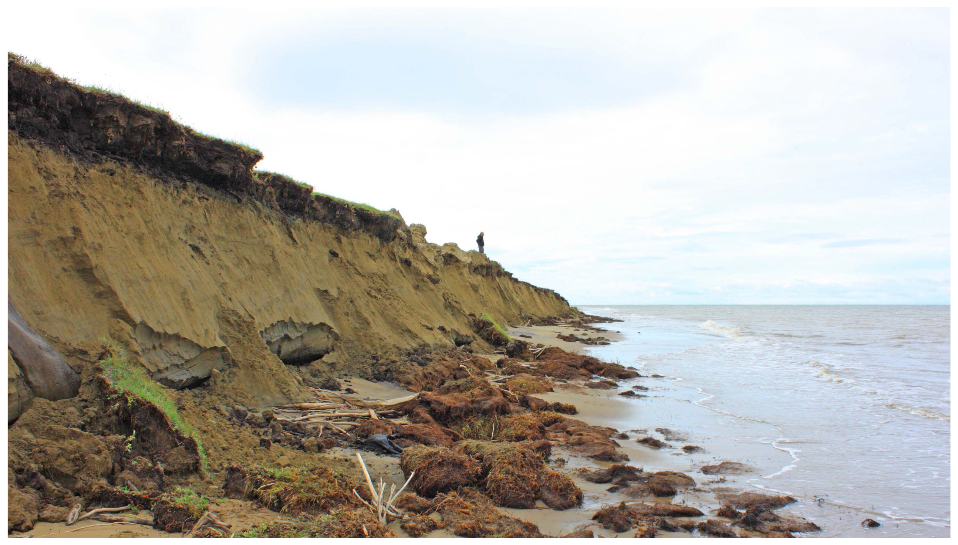
Figure 1 illustrates an example site affected by coastal erosion within the permafrost domain along the coastline of the Tuktoyaktuk Peninsula in Canada.
This highlights the need for large-scale and high-resolution quantification of Arctic coastal change in order to fully assess the impacts of eroding permafrost coastlines not only on the environment, but also on human infrastructure and society. Satellite remote sensing is hereby a powerful tool for fast, inexpensive, and spatially explicit analysis over large spatial scales [
40]. It is particularly valuable for analyzing remote and difficult-to-access regions. However, challenging environmental conditions in the form of low sun angles, frequent cloud cover, and low light intensities (including polar night) limit the usability of optical data in Arctic environments [
41,
42]. Synthetic Aperture RADAR (SAR) data on the other hand is largely independent of the aforementioned environmental conditions and serves therefore as a very attractive data source for studying these regions [
43]. Bartsch et al. [
44] investigated in a recent study the applicability of different SAR wavelengths in the context of detecting coastal erosion. Although the general application was rated to be feasible, issues with viewing geometries, inconsistencies in data acquisition, and ambiguous scattering behavior proved to be considerable challenges [
44]. Another recent study by Philipp et al. [
40] demonstrated a significant reduction in noise within the backscatter signal by working on annual composites instead of single observations.
First efforts in circum-Arctic erosion quantification were made by Lantuit et al. [
14], who provided a geomorphological classification for 1315 segments covering over 100,000 km of Arctic coastline in the form of the Arctic Coastal Dynamics Database (ACD) database. Next to the coastal change rates, the database also provides information about parameters, such as shore material, volumetric ground ice content, soil organic carbon content, and several others [
14]. A recent study by Rolph et al. [
45] presented the first physics-based model to simulate coastal retreat rates at the circum-Arctic scale, called “ArcticBeach v1.0”. Simulated coastal erosion was thereby in the same order of magnitude as the observed erosion rates based on two test sites [
45].
This study aims to build a comprehensive monitoring framework for current and future coastal erosion on a circum-Arctic scale and high resolution based on satellite remote sensing data. It therefore aims to close existing gaps by providing an inexpensive, robust, reproducible, and ongoing observation approach with high spatial resolution (10 m) on an annual basis. It hereby further represents the logical continuation of the recently published work by Philipp et al. [
40] through the application of the same methods on a circum-Arctic scale. Thus, the goals of this study are (1) to generate a high quality and circum-Arctic coastline product using a Deep Learning (DL) workflow in combination with annual Sentinel-1 (S1) backscatter composites, and (2) to quantify pan-Arctic erosion and build-up rates with high spatial resolution via a Change Vector Analysis (CVA) approach. In addition to manually digitized reference data, the OpenStreetMap (OSM) coastline was used for training the DL networks. Although quality fluctuations across different regions are frequently reported for OSM [
40,
46], the vast amount of additional training data outweighs the variations in data quality for neural networks, which are reported to be comparatively error resistant [
47,
48].
2. Materials and Methods
The study was generally divided into three parts. First, the study area was selected and S1 Ground Range Detected (GRD) backscatter images in Interferometric Wide (IW) swath mode were pre-processed. Annual median and standard deviation (sd) backscatter composites were generated for the years 2017–2021. Annual composites represent the months June–September. The second step was dedicated to the generation of a DL-based high quality and circum-Arctic scale coastline product which acted as a basis for all further analysis. Nine different U-Net architectures have been combined to generate a DL-based coastline product covering a total of 161,600 km of the Arctic coastline. Lastly, coastal change was quantified in proximity to the DL reference coastline via a CVA approach in combination with the annual S1 backscatter composites. In addition to the DL coastline and the CVA-based coastal change quantification, several quality layers were provided to assess the applicability of the proposed data and methods across different regions, and for quality control of the final output products. In addition, the impact of tidal changes on the analysis was investigated. Changes in local tides may have a significant influence on the exact location of the transition zone between land and sea, especially for flat sandy coasts. Each processing step and product are described in detail in the following sections.
A variety of data from different sources were used throughout this study. Mainly, S1 GRD images in IW swath mode [
49] were applied for the analysis. Imagery from Sentinel-2 (S2) [
50] and Google Earth [
51] acted as a means for additional quality control. In case of Google Earth, high-resolution imagery from Maxar Technologies and Centre national d’études spatiales (CNES)/Airbus were available. Furthermore, the Climate Change Initiative (CCI) permafrost fraction dataset by Obu et al. [
52] as well as the Arctic coastline product derived from OSM [
53] served to define the study area. Moreover, Mean Tidal Level (MTL) information by the National Oceanic and Atmospheric Administration (NOAA) [
54] from four buoy stations were incorporated to study the impact of tidal changes on the proposed methods and data. Further quality control was achieved through the Global Land Ice Measurements from Space (GLIMS) glacier database [
55] and information about daily sea ice concentration via the ARTIST Sea Ice (ASI) dataset [
56]. Lastly, the coastal erosion rates based on the proposed data and methods in this study were compared to coastal change information provided in the ACD by Lantuit et al. [
14]. Details on the applied data, such as the data type, spatial and temporal resolution, as well as temporal coverage within this study are listed in
Table 1.
2.1. Study Area
The first major part of this study was dedicated to the selection of the study area. It is limited to Arctic coastal areas in proximity to permafrost occurrences and with available S1 GRD imagery in IW swath mode. The Arctic coastline product from OSM was used as the basis as it proved to have the highest overall accuracy compared to other publicly available coastline products across 10 test regions in the Arctic [
40].
As a first step, the CCI permafrost fraction for the year 2017 by Obu et al. [
52] was used to define the extent of permafrost. The data were converted into a binary map where pixel values are either 0 (no permafrost) or 1 (≥1% permafrost occurrence). In order to also include smaller islands in proximity to the coastline that are not covered by the dataset, a buffer of 20 km was computed around the binary map.
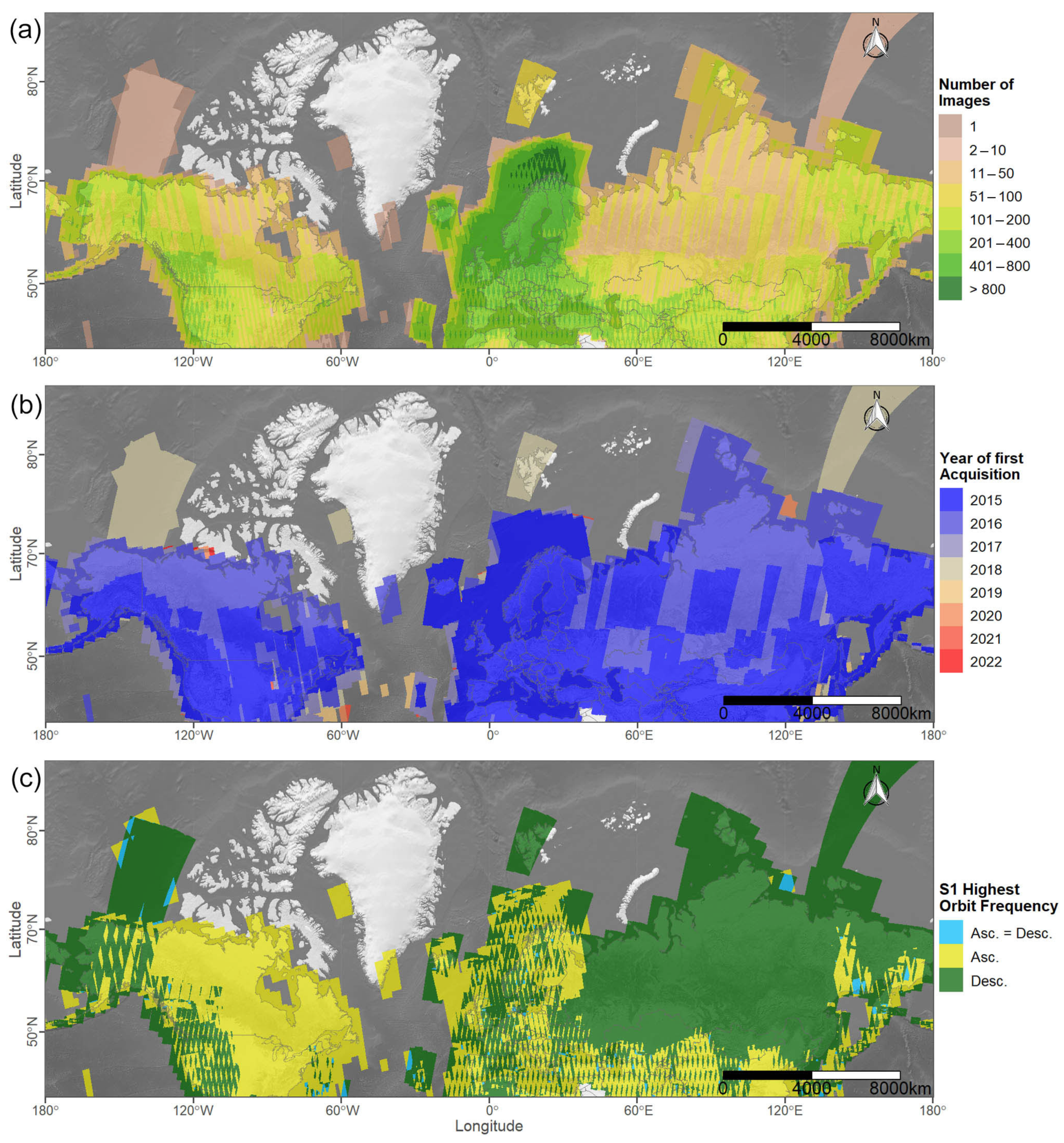
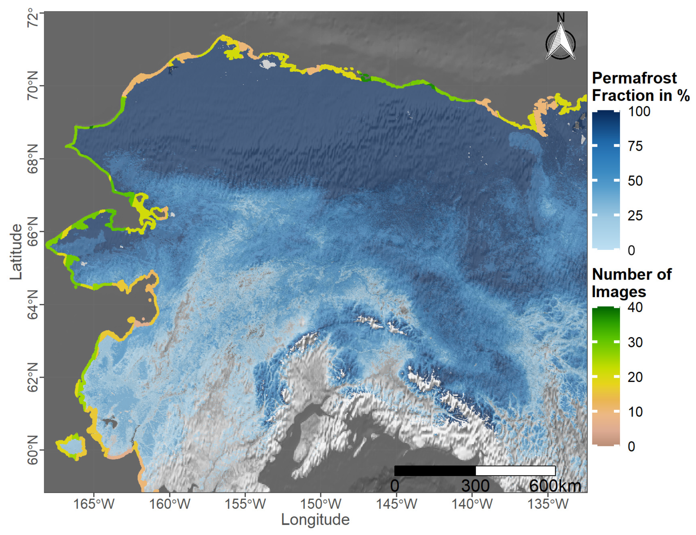
The next step was to assess the spatio-temporal availability of S1 satellite imagery. For this purpose, the number of all S1 GRD imagery in IW swath mode for the months June–September and until the end of the year 2021 from 30 degrees latitude upwards was computed on a pixel basis (
Figure 2a). Data access and filtering were conducted in Google Earth Engine (GEE). We further differentiated between imagery with an ascending or descending orbit. Based on the data frequency per orbit, a categorical map was defined that shows which orbit features the highest amount of S1 scenes per pixel (
Figure 2c). This map served as a basis for any further processing of S1 data to make sure the most frequent orbit was used when filtering the data. If both orbits feature the same amount of images, S1 data were filtered to the ascending orbit. Moreover, the year of first available data per pixel is portrayed in
Figure 2b. A binary for areas with one or more images present was created.
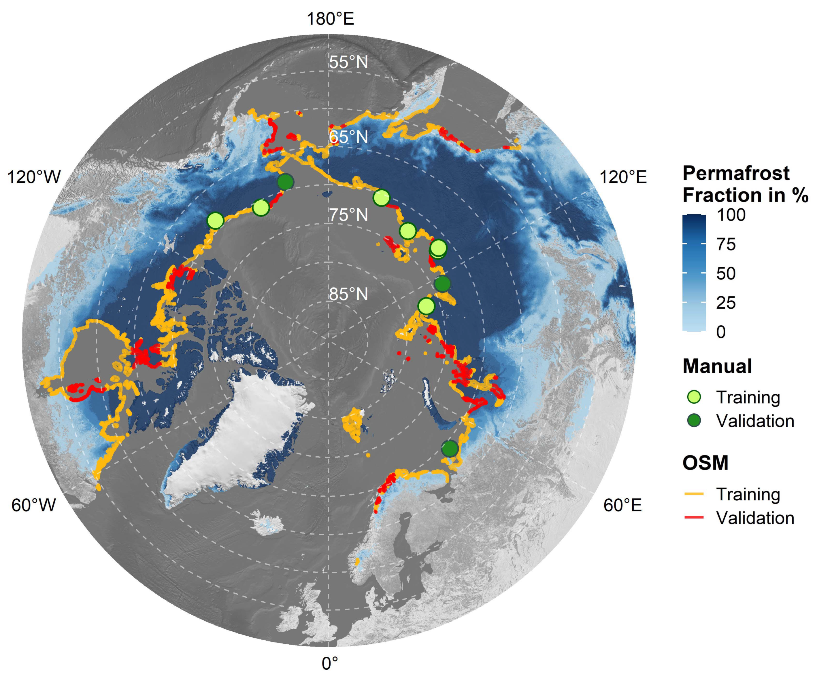
As a last step, the OSM Arctic coastline product was clipped to the binary maps of permafrost occurrence and S1 data availability to reveal the investigated coastline (
Figure 3). A buffer of 10 km was applied on the clipped coastline in order to account for any potential inaccuracies of the OSM product.
2.2. Framework for Deep Learning-Based Arctic Coastline Extraction
The application of DL Convolutional Neural Networks (CNNs) has become increasingly popular in recent years and several studies testify to its capabilities, especially in the context of land vs. water segmentation [
59,
60,
61,
62]. One major objective of this study is to take advantage of the DL segmentation capabilities in order to generate a high-quality and circum-Arctic coastline product. The feasibility of combining S1 SAR data with a U-Net-based segmentation algorithm was already demonstrated by Philipp et al. [
40]. In this study, the same concept is applied on a circum-Arctic scale with additional training via OSM as reference data. A detailed overview of how a CNN-based U-Net structure works is given by the previous publication by Philipp et al. [
40] and in the original paper by Ronneberger et al. [
63].
2.2.1. Preparation of Sentinel-1 Pseudo-RGB Images
SAR data were derived from S1 features continuous observation capabilities due to its nature of being largely independent of sun illumination and weather conditions [
43,
64]. For that reason, S1 Level-1 GRD backscatter imagery in IW swath mode was employed for this study. The satellite data is available as backscatter coefficient sigma nought (
) in the unit decibel (dB) with a spatial resolution of 10 m and was accessed via the cloud computing platform GEE [
65]. Imagery for the year 2020 and for the months beginning of June until the end of September was selected. Scenes between June and September were chosen to reduce the influence of sea ice contamination. The data were filtered to the most frequent orbit for a given region based on the previous data availability analysis (
Figure 2c). The amount of speckle in each scene was reduced by applying a 3 × 3 median Moving Window (MV). Images were temporarily converted from dB to natural for the removal of speckle. As a next step, median and sd backscatter images for each polarization, vertical-horizontal (VH) and vertical-vertical (VV), were computed. While the median backscatter tends to be generally lower over water compared to land, the opposite effect can be observed for the sd backscatter. Here, the sd backscatter proved to be higher over water and lower over land [
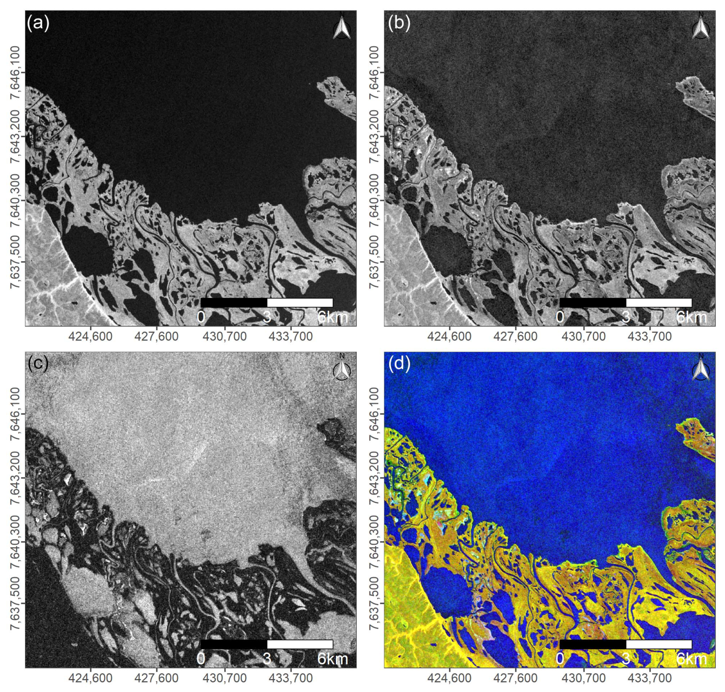
40]. This information was utilized to create Pseudo-Red Green Blue (RGB) images, with the median backscatter in VH polarization as the red channel, median backscatter in VV polarization as the green channel, and sd backscatter in VV polarization as the blue channel. Each scene was further normalized to their 2nd and 98th percentile.
Figure 4 visualizes each of the channels, as well as the combined Pseudo-RGB for an example region in Shoalwater Bay, Canada. These Pseudo-RGB images served subsequently as inputs for training the U-Net models. In addition to the Pseudo-RGB images, the number of available scenes on a pixel basis was extracted as a quality layer for the final DL coastline product. All data access, filtering, and pre-processing were conducted in GEE.
2.2.2. Preparation of Training and Validation Data
Training and validation data were collected on two levels. In the first level, a total of 1038 km of Arctic coastline and a combined area of 19,275 km
split into ten different regions across the Arctic were manually digitized. Details on the digitization process and the individual regions can be found in Philipp et al. [
40]. Each region was associated with significant erosion rates based on the ACD by Lantuit et al. [
14] and was therefore selected as a study area. The final data in the form of binary images (1 = land; 0 = water) was split into seven regions for training and three independent regions for validation. Therefore, spatial auto-correlation between the train and test dataset could be avoided.
The second level was dedicated to generating further training and validation data based on OSM. In order to cover the variety of different coastal morphologies and to overcome the limitation of CNNs requiring a vast amount of training data, OSM was utilized as an additional reference source. OSM is one of the biggest Volunteered Geographic Information (VGI) projects and currently features over eight million contributors [
66]. Data in OSM is derived from multiple different sources and imported and edited by various editors [
46]. The quality of imported data strongly depends on the source of the created geometries, such as aerial images or Global Positioning System (GPS) traces [
46,
67]. Multiple companies including Microsoft Bing, Yahoo!, and Aerowest provided (temporal) access to their aerial image database for the OSM project [
46]. Although the overall quality of the OSM proved to outperform other freely available Arctic coastline datasets, the accuracy of the data also varies across different regions [
40]. Furthermore, although being updated regularly, the dataset may not accurately depict the current state of highly dynamic regions, e.g., changing Arctic coastlines. Having that said, the vast amount of additional data is assumed to outweigh the variations in data quality, especially when working with CNNs. For this purpose, OSM land polygons were downloaded for all areas within the study region that are not already covered by the manually digitized study areas. The polygons were subsequently converted to binary rasters where pixel values are 1 in the case of the terrestrial area and 0 in the case of the water area. The entire OSM reference dataset was split into 136 tiles, of which 27 tiles were randomly chosen for validation and the remaining 109 tiles for training.
Figure 3 visualizes all training and validation data derived from manual digitization and from OSM. The previously generated Pseudo-RGB images in combination with the binary reference rasters from both the manual and OSM sites were subsequently used as inputs for training the U-Net models.
2.2.3. Deep Learning Coastline Detection
A total of nine different models were trained and their results were combined in order to perform a high-quality segmentation between sea and land areas (including inland rivers and lakes). Each of the following models ResNet34 [
68], ResNet50 [
68], VGG16 [
69], VGG19, [
69], Inception v3 [
70], Inception-ResNet v2 [
71], DenseNet121 [
72], ResNeXt50 [
73] and SE-ResNeXt50 [
74] were available with pre-trained encoder weights based on the ImageNet database (≈14 Mio. images).
Additional model training was conducted in two stages. First, reference data from the manually digitized sites were utilized to train each model. The input data were converted to tiles the size of 512 by 512 pixels. A total of seven augmentations were applied to the input data, resulting in 49,096 tiles (32,606 tiles for training; 16,490 tiles for validation). As for the hyper-parameters, a Root Mean Square Propagation (RMSprop) optimizer with a learning rate of 0.001, a batch size of 8, a binary cross-entropy loss function, and binary accuracy as an accuracy metric were used. Each model was trained for 30 epochs. The number of epochs describes how often the entire dataset is presented to the network for training. The epoch with the highest binary validation accuracy was hereby treated as the representative trained model.
Each of the representative models received further training in the second stage by using reference data from the OSM sites. In the case of the OSM reference data, no augmentation was applied. The number of 512 by 512 pixels tiles from OSM hereby totaled 307,056 (237,460 tiles for training; 67,760 tiles for validation). The same hyper-parameter settings were applied for the training with data from manually digitized sites. Again, the models were trained for 30 epochs, and the epoch with the highest binary validation accuracy acted as the representative output per architecture.
The fully trained models were subsequently utilized to create probability maps with values ranging between 0 and 1 for each 512 by 512 pixels tile across the entire area of study. A threshold of 0.5 was applied on each probability map to differentiate between land (including inland rivers and lakes) and sea area. As a result, nine binary maps, one from each model, were available per tile. In order to receive the most representative output class, the mode value was computed across all nine binary segmentation maps on a pixel basis. In addition to the mode, the (dis-)agreement between the models was assessed as a quality layer for the DL-based final coastline product. The formula for the normalized model agreement is shown in Equation (
1). The value ranges between 0.11, if only 5 out of 9 models agreed on the output class, and 1, if the output of all models was the same class. Lastly, objects that are smaller ≈0.2 km
were removed, and holes that are smaller ≈3 km
were closed in the final binary classification map. The border between sea and land area (including inland rivers and lakes) was vectorized, revealing the DL-based coastline product. A final screening of the coastline product was conducted and minor local adjustments were manually applied.
where:
= Number of occurrences of the mode value;
= Total number of models;
= Total number of classes.
2.3. Quantification of Coastal Change
As described in detail by Philipp et al. [
40] and as shown in
Figure 4, median backscatter and sd backscatter tend to show inverse behavior when comparing land and water areas. While the median backscatter is generally higher over land and lower over water, the opposite can be observed for the sd backscatter. This behavior can be exploited to analyze changes between land and water via a CVA approach. CVA is a commonly applied tool in change detection analyses and allows not only for the identification of the change direction, but also the magnitude of change [
75]. Furthermore, CVA avoids an accumulation of errors from separate input classifications in contrast to traditional post-classification change detection approaches [
76]. Therefore, CVA in combination with S1 backscatter was employed to quantify coastal change on a circum-Arctic scale.
2.3.1. Magnitude of Change via Change Vector Analysis
In order to conduct the CVA, annual median and annual sd backscatter for the years 2017 and 2021 were computed. For areas where no images were available for the year 2017, scenes from 2018 were used instead. Similar to the pre-processing of Pseudo-RGB images, S1 GRD scenes in IW swath mode were filtered to both years and to the months June–September. Images were further filtered to the most common orbit per area based on the previously calculated orbit frequency map (
Figure 2). Moreover, the speckle effect was reduced by applying a 3 × 3 median MV. Lastly, median and sd backscatter in VV polarization was computed for each year and used as inputs for the CVA computation. If the median backscatter decreased and the sd backscatter increased, it was interpreted as a change from land to water and thus, erosion. If a change in the opposite direction could be observed, it was interpreted as build-up. The final magnitude of change maps was normalized to have values ranging between 0 and 1. Moreover, the number of available images per year and per pixel were assessed as an additional quality layer for the final CVA coastal change product.
2.3.2. Post-Processing of Change Vector Analysis
The previously computed DL coastline product served as a reference area for the coastal change analysis. A one-sided buffer with a size of 200 m was computed in the direction of the sea, while a 50 m buffer was added in the direction of land. The magnitude of change maps was clipped to the buffered coastline area in order to limit the change detection to the coastline. Next was the identification of suitable thresholds for differentiating between actual change and noise within the magnitude of change maps. For this purpose, manual delineation of coastal change was conducted for the manual test sites based on the analyzed S1 scenes in combination with optical data from S2 and high-resolution imagery from Google Earth. These manually digitized coastal changes served as a reference for identifying the most suitable threshold values (0.35 for erosion and 0.6 for build-up). Details on creating the reference data and extracting optimal threshold values can be found in Philipp et al. [
40]. A 3 × 3 mode MV was applied on the thresholded change maps to reduce the amount of left-over noise to a minimum. Further processing included computing the distance between each erosion/build-up cluster and the DL reference coastline. Clusters of coastal change with a minimum distance larger than 100 m to the DL coastline were interpreted as noise within the water and therefore removed. Moreover, the effect of changing glaciers on the analysis was reduced to a minimum by removing areas that intersect with a 500 m buffer around any glacier polygons derived from the GLIMS glacier database [
55,
77]. Moreover, areas with less than ten available S1 GRD scenes in IW swath mode in either the year 2017 (or 2018) and/or 2021 were excluded from the analysis. Within the context of this study, it is assumed that a higher amount of available images generally leads to more robust change analyses. Therefore, and to avoid measuring noise instead of change, only areas with more than 10 scenes available for the months of June–September in both years were included. Furthermore, areas with less than 50% sea-ice-free days in either year during the observation period June–September were excluded from the analysis. A pixel was considered contaminated by sea ice if at least 20% ice was present based on daily sea ice concentration information from the ASI database [
56]. Finally, average change rates in the form of erosion and build-up were computed separately for 400 m segments along the DL coastline. For each segment, a rectangular polygon the size of 40 × 40 pixels (400 × 400 m) around a center point on the coastline was generated. Next, the number of erosion/build-up pixels in this area was extracted. Lastly, the average change (either build-up or erosion) per segment could be calculated as shown in Equation (
2).
where:
= Average change (either erosion or build-up) per segment in meters;
= Length of the rectangular observation window in meters;
= Number of pixels that indicate change (either erosion or build-up);
= Total number of pixels in the observed window.
2.4. Validation and Quality Control
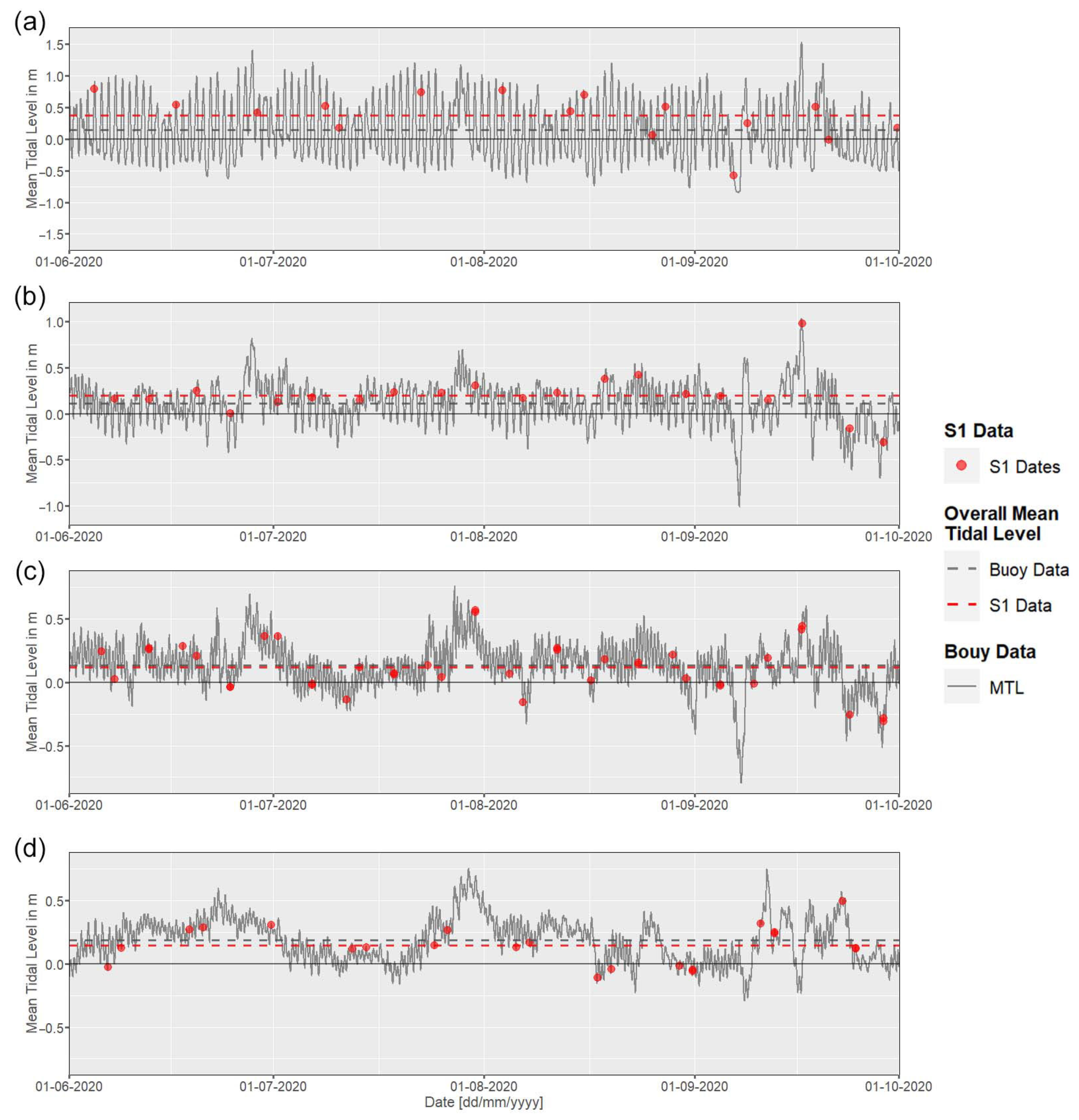
Extensive efforts were made for validating both the DL coastline product and the CVA coastal change analysis. Next to accuracy statistics based on manually digitized reference coastlines, quality layers, such as the model agreement, the number of available images, and the total number of days with sea-ice contamination during the observation period are provided on a pixel basis. Further analysis of the impact of tidal changes on identifying the coastline was performed.
2.4.1. Tidal Influence on the Accuracy of the SAR-Based Coastline
The exact delineation of the Arctic coastline may vary throughout the observation period June–September due to tidal changes. Therefore, it is reasonable to not use single observations, and instead combine several images across an observation period to receive a representative output. However, based on the number of available images on the current tide level at the acquisition times, the quality of this aggregated image may vary. In order to assess the impact on tidal changes, MTL from four buoy stations on a six-minute basis and covering the same temporal window as the Pseudo-RGB images (June–September 2020) provided by the [
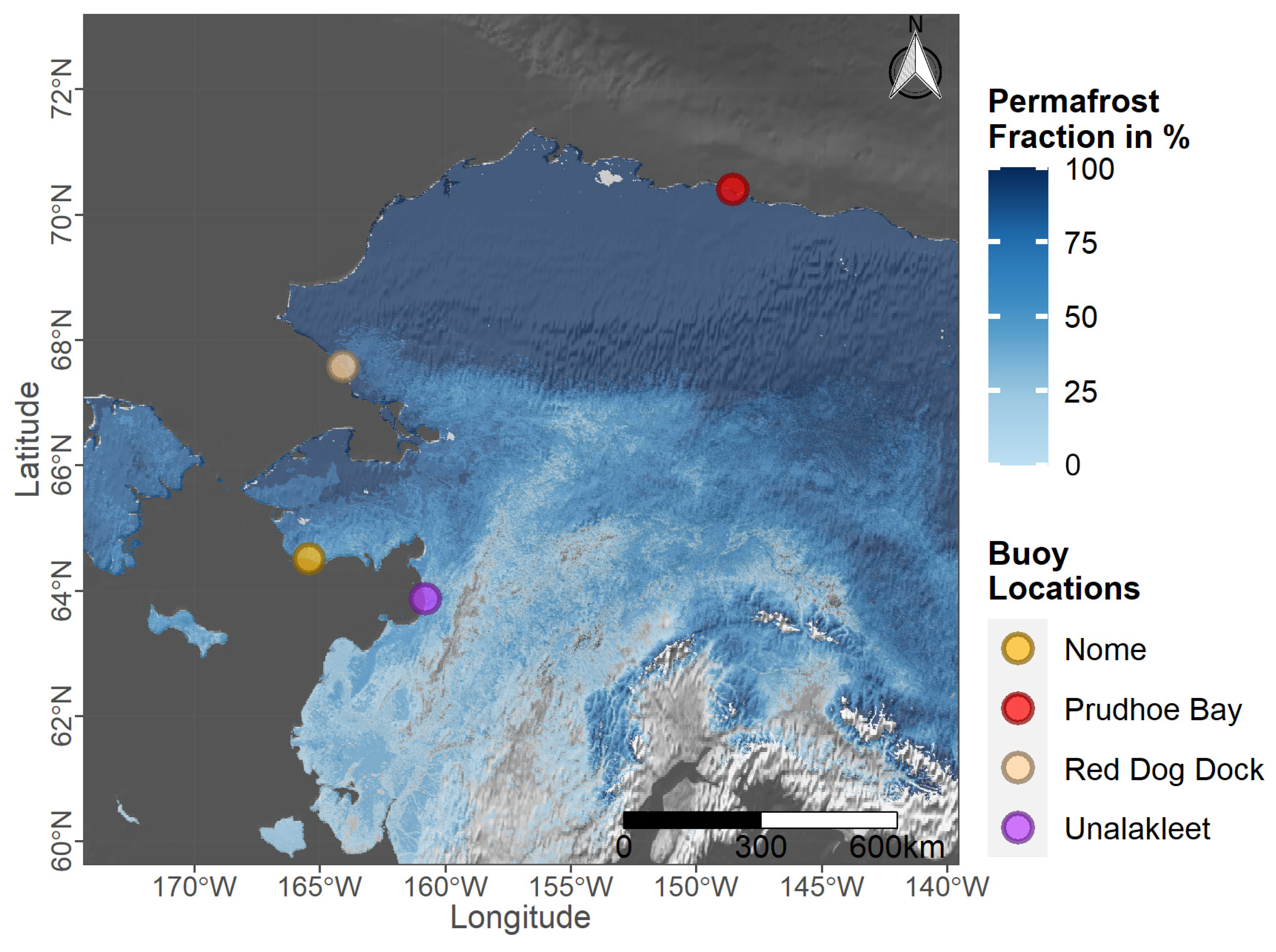
54] were downloaded. MTL data from the following stations were used: 9468333 Unalakleet, 9468756 Nome, 9491094 Red Dog Dock, and 9497645 Prudhoe Bay.
Figure 5 illustrates the distribution of buoy stations across Alaska.
The MTL describes the arithmetic mean of mean high water and mean low water [
78]. The MTL for each acquisition date and time of available S1 GRD data in IW swath mode was extracted for each tide station and compared to the overall mean MTL across the entire observation period. It was ensured that both satellite data and buoy data are present in the same time zone (Greenwich Mean Time (GMT)). It is assumed, that a close mean MTL from S1 acquisition dates to the overall mean MTL across the entire observation period indicates a highly representative annual S1 composite.
2.4.2. Accuracy Assessment of Deep Learning Coastline
Statistics on the binary accuracy and loss values for each model are provided for the quality assessment of the individual model outputs. In addition, further accuracy assessment on the final combined binary classification map within a 500 m buffer around the coastline was conducted. Since high accuracy numbers can be expected for binary classifications across large regions, a focus was put on the transition zone between land and sea area. For this purpose, common metrics, such as overall accuracy, precision, recall, and the
-score were derived. We differentiated between training and validation areas, as well as between manually digitized sites and OSM sites. The deviation between the 1038 km of manually digitized reference coastline and the generated final DL coastline product served as another means to quantify the quality of the predicted coastline. Moreover, several quality layers are available, such as the number of available S1 scenes, the level of agreement between the nine separate models, and the total number of days with more than 20% sea-ice contamination during the observation period via the ASI database [
56].
2.4.3. Accuracy Assessment Coastal Change via Change Vector Analysis
As for the CVA analysis, manually digitized coastal changes across the manual test sites served as a basis for suitable threshold identification. Details on the creation of reference data for the CVA change maps are provided in Philipp et al. [
40]. Moreover, the number of available S1 images, and the total number of days with sea-ice contamination based on the ASI database [
56] are provided per year and per pixel as additional quality layers. The number of days with ≥20% sea ice for the time period June–September 2017 across the Arctic is visualized in
Figure 6.
Lastly, information about the glacier extent using the GLIMS glacier database [
77] was included for quality control. The magnitude of change maps themselves act as a further quality layer that can be used to identify custom threshold values based on image availability, sea ice contamination, and region.


