Article

Identification of Streamside Landslides with the Use of Unmanned Aerial Vehicles (UAVs) in Greece, Romania, and Turkey

by
Mehmet Yavuz
1,
Paschalis Koutalakis
2,
Daniel Constantin Diaconu
3,
Georgios Gkiatas
2,
George N. Zaimes
2,*,
Mustafa Tufekcioglu
1 and
Maria Marinescu
4
1
Department of Forest Engineering, Faculty of Forestry, Artvin Coruh University, 08100 Artvin, Turkey
2
Geomorphology, Edaphology and Riparian Areas Laboratory (GERi Lab), Department of Forestry and Natural Environment Sciences, International Hellenic University, 66100 Drama, Greece
3
Ministry of Investments and European Projects, 013681 Bucharest, Romania
4
Buzau Ialomita Water Administration, 120208 Buzau, Romania
*
Author to whom correspondence should be addressed.
Remote Sens. 2023, 15(4), 1006; https://doi.org/10.3390/rs15041006
Submission received: 30 November 2022 / Revised: 21 January 2023 / Accepted: 9 February 2023 / Published: 11 February 2023
(This article belongs to the Section Earth Observation for Emergency Management)

Abstract

:
The alleviation of landslide impacts is a priority since they have the potential to cause significant economic damage as well as the loss of human life. Mitigation can be achieved effectively by using warning systems and preventive measures. The development of improved methodologies for the analysis and understanding of landslides is at the forefront of this scientific field. Identifying effective monitoring techniques (accurate, fast, and low cost) is the pursued objective. Geographic Information Systems (GISs) and remote sensing techniques are utilized in order to achieve this goal. In this study, four methodological approaches (manual landslide delineation, a segmentation process, and two mapping models, specifically object-based image analysis and pixel-based image analysis (OBIA and PBIA)) were proposed and tested with the use of Unmanned Aerial Vehicles (UAVs) and data analysis methods to showcase the state and evolution of landslides. The digital surface model (DSM)-based classification approach was also used to support the aforementioned approaches. This study focused on streamside landslides at research sites in three different countries: Greece, Romania, and Turkey. The results highlight that the areas of the OBIA-based classifications were the most similar (98%) to our control (manual) classifications for all three sites. The landslides’ perimeters at the Lefkothea and Chirlesti sites showed similar results to the OBIA-based classification (93%), as opposed to the Sirtoba site, where the perimeters of the landslides from OBIA-based classification were not well corroborated by the perimeters in the manual classification. Deposition areas that extend beyond the trees were revealed by the DSM-based classification. The results are encouraging because the methodology can be used to monitor landslide evolution with accuracy and high performance in different regions. Specifically, terrains that are difficult to access can be surveyed by UAVs because of their ability to take aerial images. The obtained results provide a framework for the unitary analysis of landslides using modern techniques and tools.

Graphical Abstract

1. Introduction

Landslides are irregular and active landforms generated by the gravitational downslope movement of rocks, soils, or both [1]. They are complex natural phenomena, generated by a wide range of factors (geology, slopes, land use, climate, etc.) and occur in different forms and types (deep earth movements, rapid landslides such as falling rocks, muddy flows, etc.) [2]. Differences in the predominant type of transported material and different deposit formations lead to many different types and categories [3,4,5,6,7]. Globally, landslide-induced losses of human infrastructure and life have substantially increased [4]. Each type of landslide has different characteristics and needs to be studied.
Of special interest are streamside landslides [8,9,10], which occur along streambanks or the adjacent steep terrain within the riparian zone; they transport soil, rock, and vegetation to stream channels and affect stream sedimentation. These are considered erosion control hot-spots because they are highly affected by the vegetation (roots) and water present in the soil. Part of a rock’s or soil’s shear strength is based on cohesion rather than interparticle friction [11]. The cohesion index is the relative contribution of soil to inhibiting the development of a slope failure through root cohesive forces; thus, along with the slope, it plays a significant role in landslides and especially in streamside landslides, which are influenced by riparian zones [12,13,14]. The primary landslide types that have an impact on streams are debris slides and flows [15,16]. These landslides impact the drainage-basin sedimentation rates since they can provide substantial volumes of transported materials from the hillslope to stream channels [17,18] and affect sediments distributed in stream channels over time and space [19]. Streamside landslides also cause major disturbances in the adjacent riparian ecosystems (geomorphic, abiotic, and biotic) [20].
The main parameters measured for a landslide to enhance the understanding of its mechanics and processes are (a) the vertical and horizontal displacements of the sliding body, (b) the pressures exerted during the landslide, and (c) the groundwater, spring, and surface water properties [21,22]. The variety of landslide types and characteristics, along with the landforms over which they take place and the accessibility of the research area, leads to the utilization of diverse monitoring equipment and technologies [23,24]. Easily identifying the areas affected by landslides, understanding their process, and monitoring them will protect the human population, reduce economic losses, and, more importantly, lead to the adoption and implementation of timely and cost-effective preventive measures [25,26].
Early warning and real-time monitoring systems have become important for landslide mitigation measures due to their efficiency with the use of affordable equipment and technologies compared to traditional ones [27,28]. New tools define the characteristics of landslide locations, provide soil conditions, and reveal the effectiveness of different mitigation methods [29]. Effective landslide-monitoring technologies require the combination of theoretical and field analyses [30,31,32,33,34]. The technologies and techniques used for landslide monitoring can be classified into three main categories: (a) statistical methods and rating schemes for landslide susceptibility hazard and zonation mapping [35,36,37,38], (b) remote sensing techniques [39,40,41], and (c) field measurement methods [4]. The first category estimates the probability of potential landslides. The second category uses sensors that record data, located away from the landslide. This category includes Synthetic Aperture Radar (SAR), which uses electromagnetic radiation to generate two-dimensional images or three-dimensional reconstructions to detect moving objects and estimate their ground velocity and positions [42]. The Laser Interferometer Space Antenna (LISA) is a ground antenna of an Interferometric Synthetic Aperture Radar (InSAR) system that receives images of the ground area, minimizing the effect of bad weather on the ability to obtain high-quality images [43]. Light Detection and Measurement (LiDAR) scans landslides to create point clouds and determine or monitor any deformations [44,45,46,47,48]. To locate active landslide areas, the global positioning system (GPS) is also being used [49,50].
Photogrammetric techniques use calibrated cameras with specific lenses and settings to monitor ground motion. These techniques are based on field measurements, specifically ground control points (GCPs), whose positions are determined periodically and represented in the GIS system [51,52]. Fiber optic (reflectometer) (OTDR) sensors are an effective monitoring technique and detect vibrations generated by ground movements but are very expensive. There has also been significant interest in Wireless Sensor Network (WSN)-based methods for landslide monitoring [53]. Utilizing images obtained by the networks, a series of algorithms are applied to improve their quality. A cutting-edge analytics tool called machine learning has been utilized to analyze large datasets, with a focus on the development of early warning systems for landslides, landslide detection using images, and landslide susceptibility assessment [54]. Object-based image analysis (OBIA) and pixel-based image analysis (PBIA) have received significant interest for mapping landslides based on the image segmentation and classification approach [34,55,56,57,58]. Their applications have increased due to the widespread use of Unmanned (or Unoccupied) Aerial Vehicles (UAVs). For the detection and monitoring of landslides, remotely sensed data (photogrammetric products) and related tools have become crucial [59]. Nowadays, UAVs have become a necessary tool in order to monitor, analyze, and measure landslides [60]. UAV-based products preprocessed with artificial intelligence technologies are very helpful for landslide detection, not only for creating susceptibility maps and inventories but also for predicting spatial landslide evolution [61]. Image cross-correlation functions and digital elevation model (DEM) subtraction techniques are applied to structure-from-motion (SfM) photogrammetric products (e.g., UAV-based orthomosaics) in order to determine the area affected by the landslide using manual delineation [62]. Different machine learning (ML) methods, for example, the multilayer perceptron neural network, K-Nearest Neighbor, random forest, and Decision Tree, have been evaluated with the inclusion of spatial, spectral, and contextual properties based on airborne or UAV-borne flights and DEMs for landslide detection [58].
Effective landslide mitigation can be achieved through the development of early warning systems, susceptibility assessments, and detection based on images [63]. The critical task at the moment is to thoroughly detect and analyze such phenomena in a timely and cost-effective manner. Despite the numerous methods proposed and tested over time, there are still constraints and gaps that affect the quality of data acquired by UAVs in this scientific field [64,65,66,67,68]. The objective of the present study was to identify hot-spots of streamside landslides utilizing UAV data on landslides in Greece, Romania, and Turkey and to improve this methodology. To achieve this objective, four different methods using images from high-tech drones were applied and tested. Initially, the drone’s images were used to produce photogrammetric products (e.g., orthomosaics and DSMs) and then analyzed in GIS to develop aspect and hillshade maps. The four methods included are (1) manual landslide delineation based on previously described products; (2) a segmentation process and two mapping models (OBIA and PBIA); (3) a showcase of the state; and (4) the evolution of streamside landslides.

2. Materials and Methods

2.1. Case Studies

This work was carried out at three different streams located in Greece, Romania, and Turkey (Figure 1). The streams selected are part of the Aggitis River Watershed (Greece), Buzau River Watershed (Romania), and Arhavi River Watershed (Turkey), all pilot areas of the Protect-Streams-4-Sea project funded by Joint Operational Programme BLACK SEA BASIN 2014-2020 (Project Number: BSB963). The Protect-Streams-4-Sea project is focused on the collaborative environmental monitoring of nonpoint source contaminants and litter that enter the Black Sea. This will be accomplished by emphasizing inland pollutants and waste, particularly those that originate from rivers and their watersheds that discharge into the Black Sea. In order to accomplish the aforementioned goals, a joint monitoring program on these pollutants and litter has been established to encourage “the coordination of environmental protection and joint reduction of pollutants and litter through the adoption of best management practices.” One of the activities is to monitor “hot-spots” of soil erosion/or deposition in the stream network of the pilot areas (e.g., landslides). Sentinel-2 satellite images were utilized to find possible hot-spots (landslides, bare soils, mines, and quarries) using the Normalized Difference Vegetation Index (NDVI), Normalized Difference Water Index (NDWI), and Normalized Difference Soil Index (NDSI) in the entire pilot areas of Buzau, Aggitis, and Arhavi Watersheds. It was difficult to determine the extent of small-sized landslides precisely due to the spatial resolution of Sentinel-2 imagery (10 m for RGB-NIR and 20–60 m for multispectral bands). To better define the landslides’ extent, UAV imagery with 1–5 cm spatial resolution was used. The studied sites are streamside landslides that have been selected as representative “hot-spots” of the entire water basins belonging to the above-mentioned pilot areas.

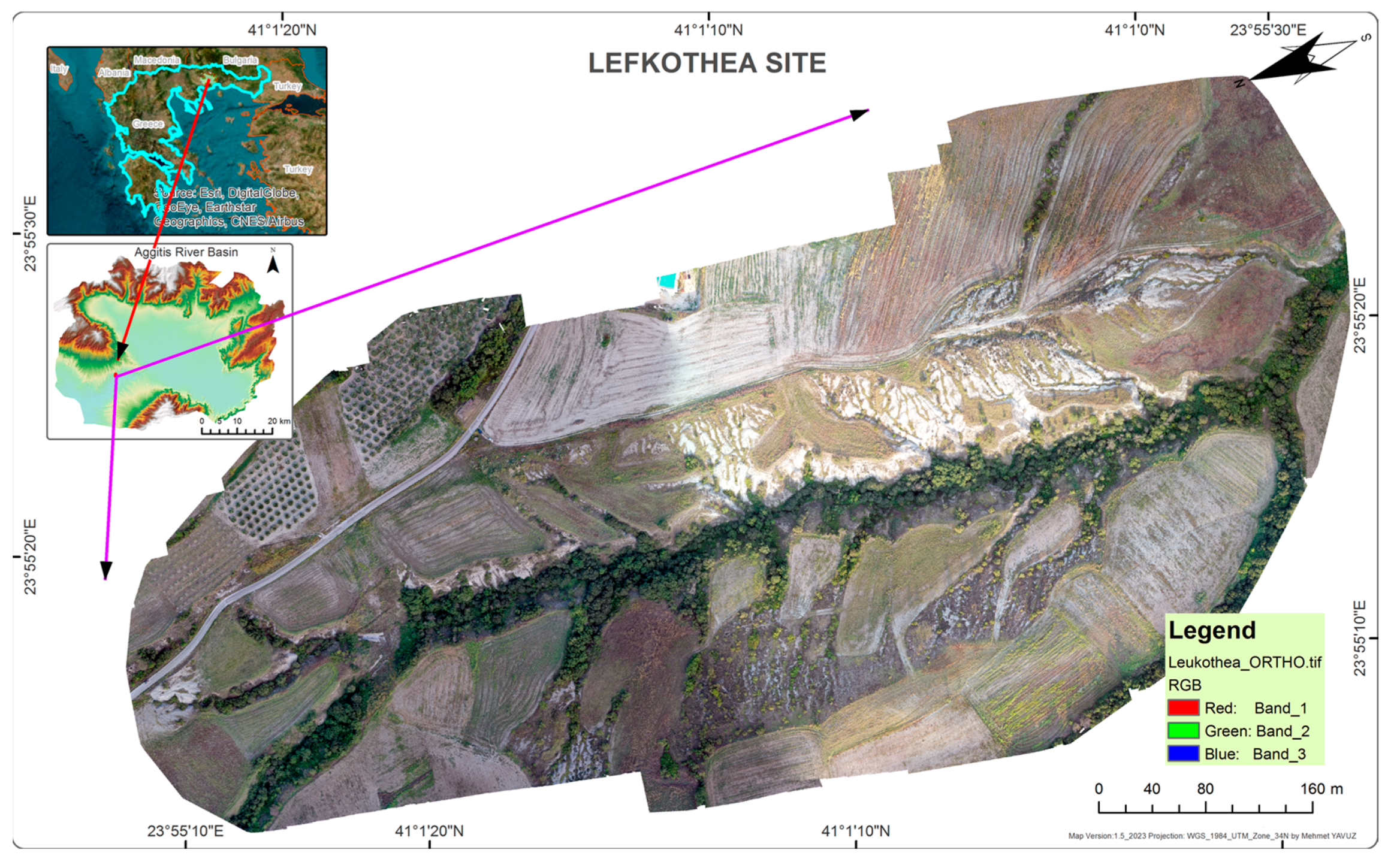
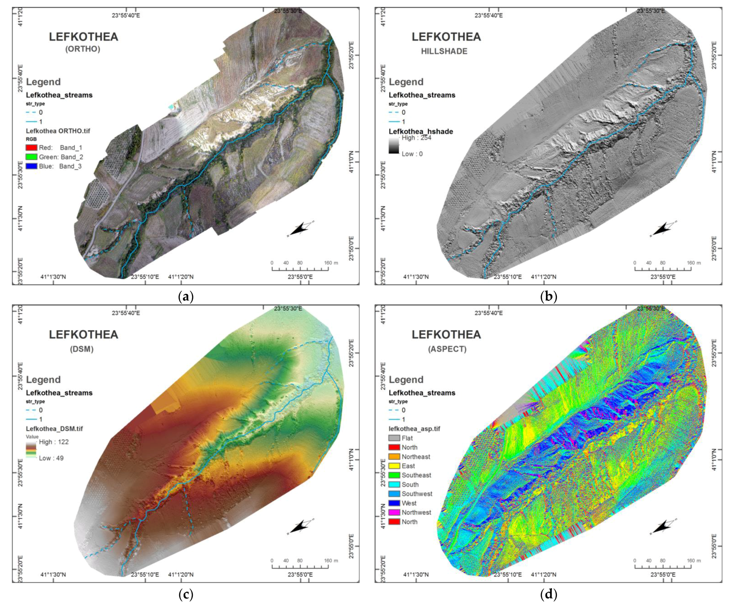
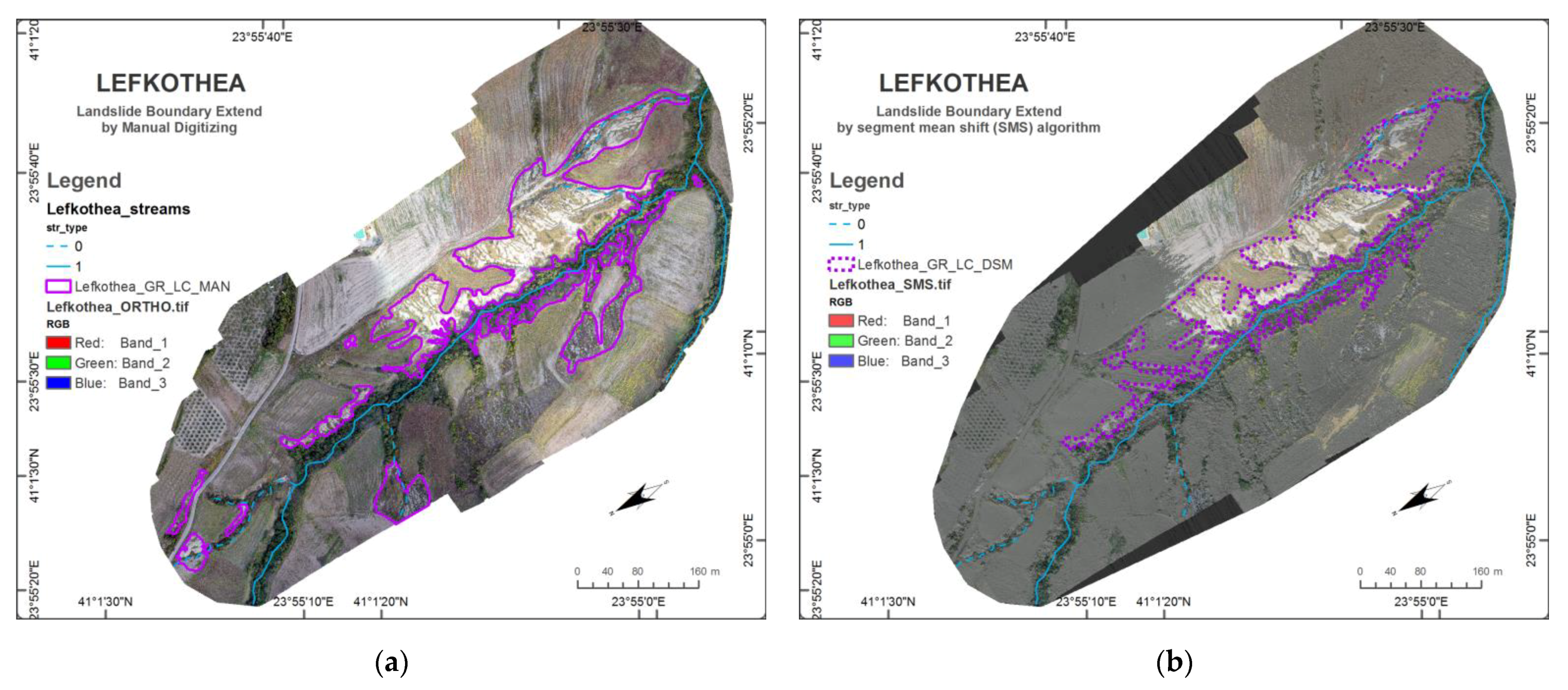
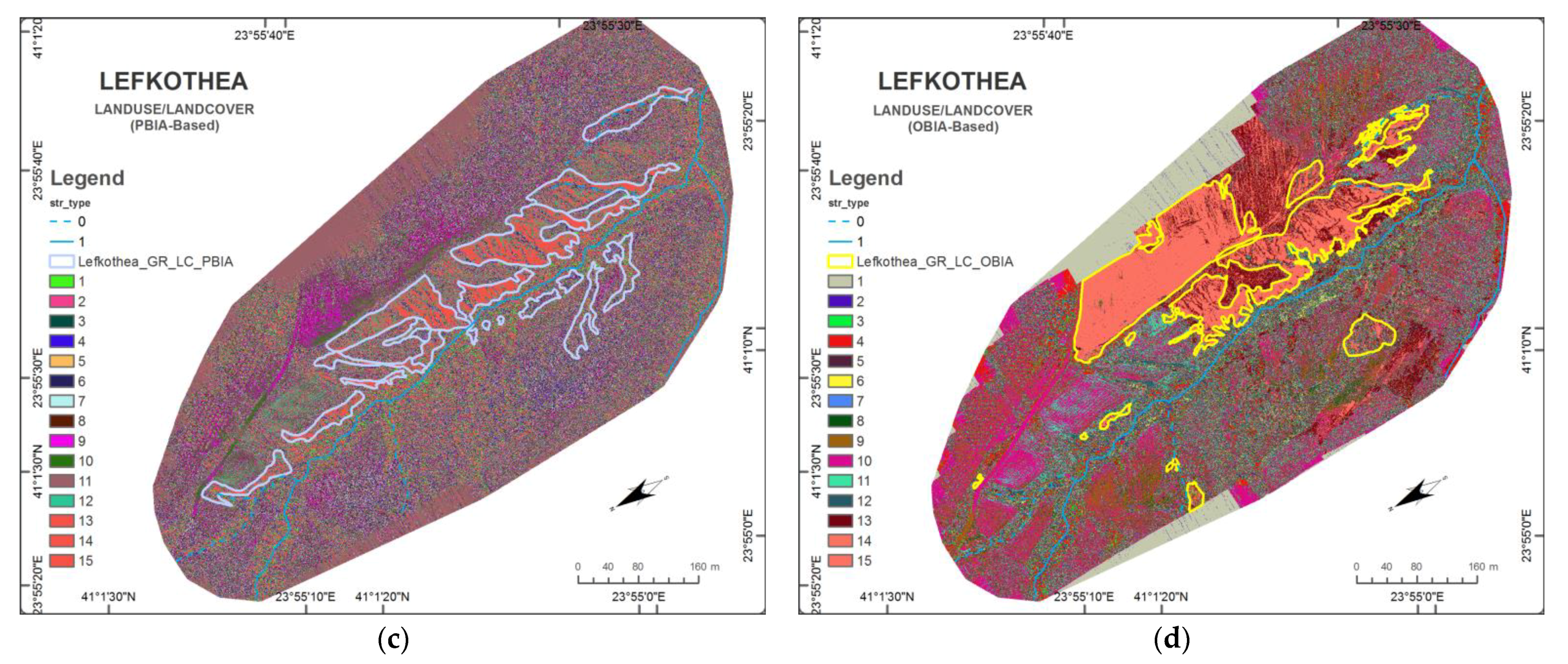
2.1.1. The Lefkothea Site of the Aggitis River Watershed (GREECE)

This case study is a torrent that is part of the Aggitis River Watershed and located near Lefkothea Village at latitudes between 41.0240° and 41.0155°N and longitudes between 23.9196° and 23.9249°E in the World Geodetic System 1984 (WGS84) (Figure 2). Aggitis River, the major tributary of the Strymonas River in the Greek territory, is 75 km long and is located in the Falakro massif and Kato Nevrokopi Plateau [69,70]. The Aggitis watershed covers an area of 2707 km2. The Menoikio Mountain, Falakro Mountain, and Ori Lekanis and Paggeo Mountains surround the watershed [71]. The stream network of the Menoikio Mountain is dominated by intermittent and ephemeral torrents [72]. The hydrographic network combines dendritic and parallel stream patterns due to the geology, geomorphology, and tectonic activity of the region [73]. In the past, the area was near the shore of Achinos Lake and its marshes, which were drained in 1932 as a result of the Strymonas River Basin’s engineering work plan [74,75]. The specific studied torrent is located at the south foothills of the Menoikio Mountain (near the Lefkothea Village), where the soils are extremely vulnerable to erosion [76]. The geologic substrate consists of a ~5 m layer of quaternary breccio-conglomerates and a ~220 m layer of silty clays, limy siltstones, and marls deposited in one monotonous clayey-limy-silty sediment with Aulacoseira fossils, representing the character of the “lake” and the Pliocene period [77]. Due to severe soil erosion, particularly in other Neogene (Miocene–Pliocene), red beds, and Quaternary sediments, the steep slopes produced numerous gullies [75,78]. The above characteristics form an intense hydrographic network with unstable slopes, while, in many locations, debris slides and gullied scarps have been recorded [79]. The preconditioning factors of the Lefkothea site are (a) regional tectonic activity with the active NW–SE-trending normal fault “Tholos–Nea Zichni” [80] and (b) the composition of the regional soils (silty clays, limy siltstones, and marls) which are extreme vulnerable to deep and intense gully erosion. The triggering factor is the extreme rainfall events that triggered the described phenomena: 80.6 mm in April 2021; 109.9 mm on 15 October 2021; and 98.2 mm on 11 December 2021, as recorded at the Micropoli weather station located in the Menoikio Mountain Range. Agricultural areas, sclerophyllous flora, natural grasslands, and broad-leaved forests make up the majority of the land cover of the pilot area, according to the locations noted in the 2018 Corine land cover data. Based on the meteorological station in Drama, the general climatic type in the Aggitis–Drama Basin has been found to be Mediterranean with hot summers (Csa) (Data 1975–2001). This comes from the fact that the driest month’s average rainfall does not exceed 30 mm (September, 22.50 mm high mean rainfall), whilst the average rainfall in the wettest month is at least three times higher than that in the driest month (56.60 mm in December). In the same manner, July, the hottest month, has an average temperature higher than 30 °C. Summer temperatures can reach 40 °C, while winter temperatures can dip to −15 °C or even lower. In the winter, the area receives high precipitation (rain and snow). The riparian vegetation is characterized as sclerophyllous with pastures and agricultural fields that are cultivated with yearly crops, and there are also a few olive orchards.

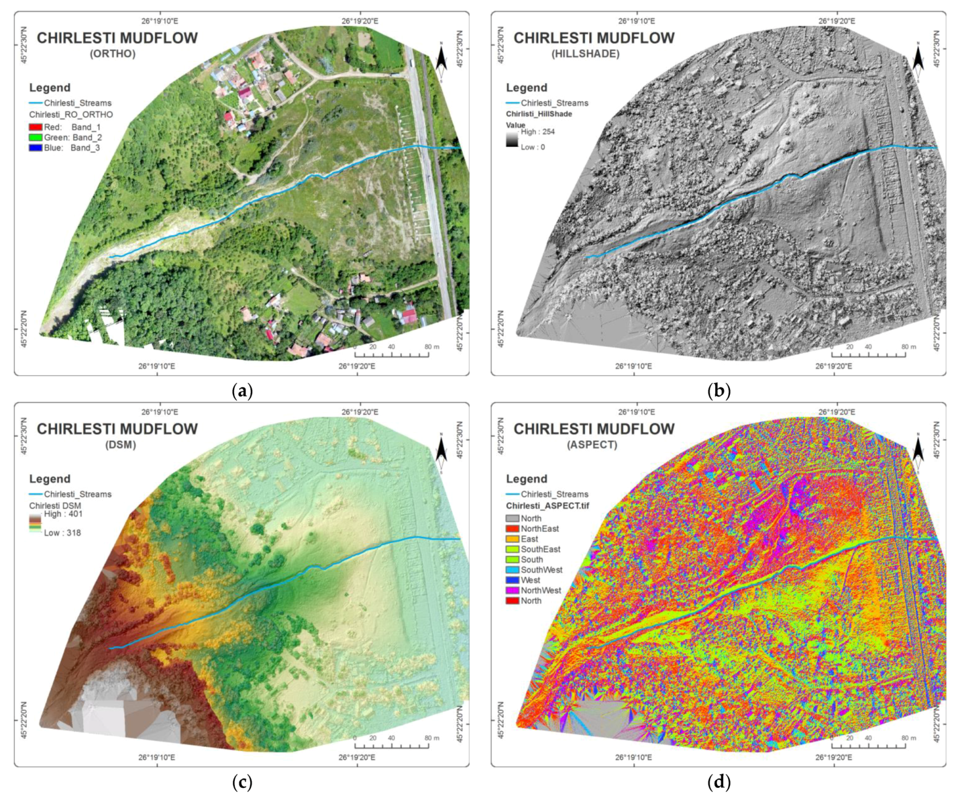
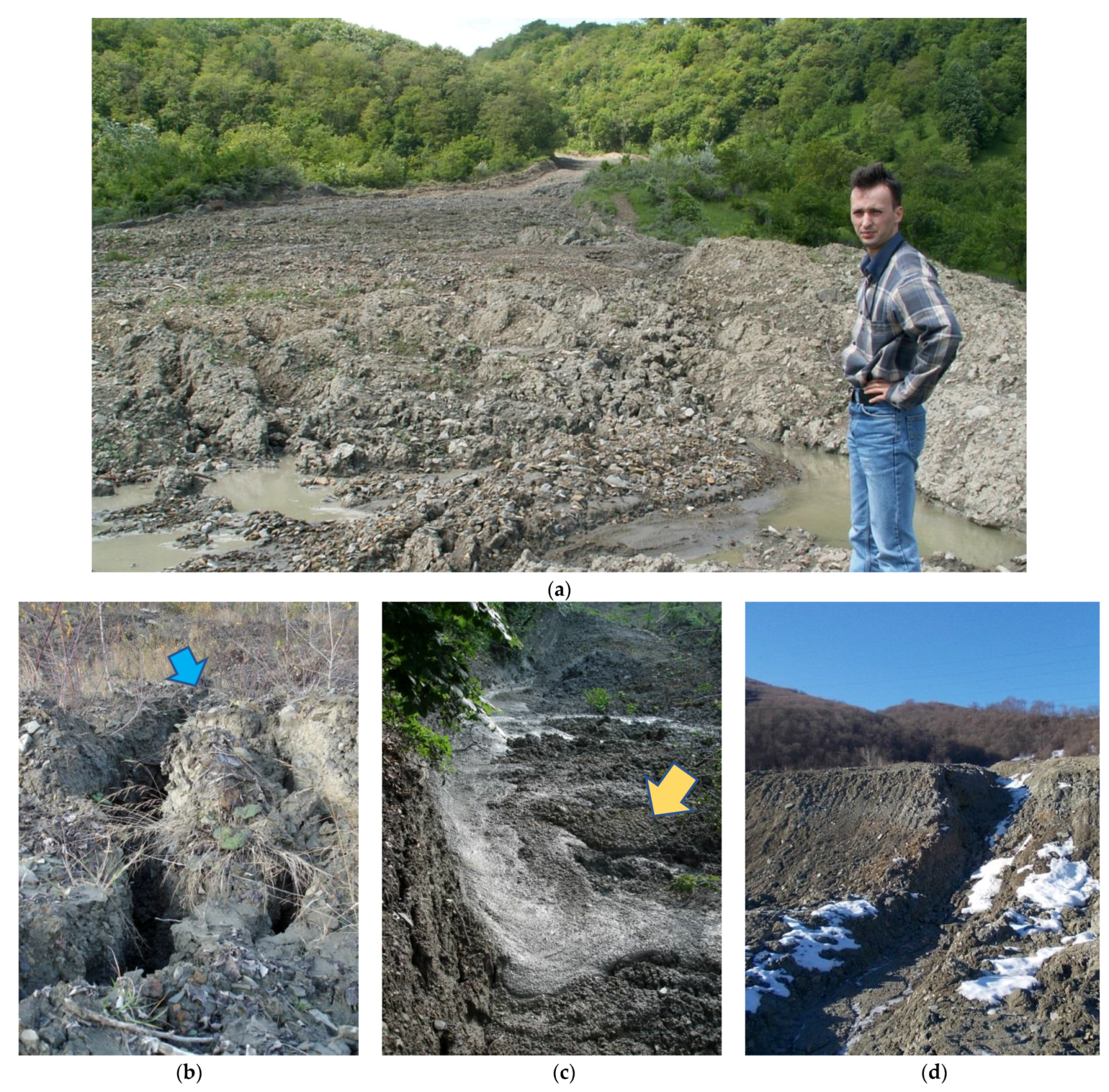
2.1.2. The Chirlesti Mudflow of the Buzau River Watershed (ROMANIA)

The landslide developed on the right side of the Buzau River at latitudes between 45.3752° and 45.3719°N and longitudes between 26.3178° and 26.3240°E in the WGS84 geographical coordinate system, within the structural curvature of Sub-Carpathians, along a valley oriented SW–NE (Figure 3) [81]. The mountainous area consists of a folding flysch aligned in the north direction. The flysch series is made up of fine sandstones that are curbicortical, micaceous, calcareous, and gray and alternate with gray clays and marls (they can be found in Zabrataului and the Siriului Mic valleys at Crasna), and 600 m thick conglomerate covers the entire formation. This lithological formation dates from the Late Cretaceous to the Paleogene Period. The region into which the upper Buzău basin drains belongs to the crystalline-Mesozoic region, as well as the Cretaceous and Paleogene flysch region. Late Cretaceous black shales are found in the region that extends from Siriu, crosses the Buzău river near Crasna, and moves north. It was grafted over Eocene deposits of gray-green claystone interspersed with thin grayish layers. The direction of the dip of the layers is SW–NE, parallel to the direction of the flow, and there is also a dislocation line between the Eocene and Oligocene [82]. Currently, the landslide has a length of 1300 m, occurring between 320 and 620 m. The high slope (about 30 degrees), high water infiltration, the foundation structure, and the composition of the sliding mass are the main factors triggering the phenomenon [83]. Due to the major source area’s exceptionally vast extent and highly heterogeneous rock formations (rich clays, sandy clays, sands, and marls), water from nearby water tables and precipitation can infiltrate quickly. As a result, the oversaturated soil starts to migrate downward as a mudflow. The accumulating colluvial mass is the result of shallow slides, granular topples, and medium- and deep-seated slumps. Sheet wash, rill erosion, and surface slides all affect the colluvium [3,84].
The average annual precipitation is between 800 and 1200 mm/m2 with a wet climate from April to September. The slopes of the watershed are covered mostly by deciduous forests (dwarf willow, rhododendron species), juniper species, pastures, meadows, and a small proportion of ace roads and houses. The agricultural lands had 18% coverage. The transported material has a heterogeneous, marno-clay structure and is very wet, with the transported matter including trees uprooted from the forested slopes. In longitudinal profiles, grain-size fractions are not very well separated, maintaining their heterogeneous character both in catchment areas and along the flow-track [85]. The catchment and alluvial basin, located at altitudes of 550–605 m, are covered by grassland. The water discharge decreases the cohesion index of the soils, triggering the failure mechanism that causes streamside landslides that can also lead to mudflows. Mineral and plant waste particles (tree trunk remnants) can be seen on the debris fan’s surface. These come from the middle area of the torrent, where landslides affect steep slopes. The flow channel has a considerable length of over 700 m and a width at the top and bottom of about 30 m. For most of its length, the channel does not exceed a width of 20 m. In terms of its appearance, the channel has a transverse profile in the form of a “U”, with the thalweg covered over its entire length by moving alluvial deposits. The material, which can reach a thickness of 1–3 m, has high moisture content, especially below 480 m, where new springs appear. The debris fan is spectacular in its development, with an altitude range of 320–350 m, a length of roughly 200 m, and a width of 250–300 m. As it slides from the top, the majority of the transported material is stored here. The material in the spreading cone is also affected by the upper part through surface washing and even surface erosion, leading to the appearance of gutters and small ravines that can exceed 1.5 m in depth. Its mobility is significant, being mainly influenced by the amount of rain falling and temperature variations. The velocity of the mudflow’s motion has seasonal differences. The spring–summer interval records the most intense dynamics (due to intense precipitation) and varies between 5 and 17 m/month with a mean value of 9.2 m/month, while winter is the most stable season, with a mean displacement velocity of 4.8 m/month [85]. Extreme temperatures promoted water evaporation (drought), which generated more cracks in the soils at the Chirlesti mudflow site in Romania. Then, surface runoff water infiltrated deep into the soil through these cracks, causing rapid soil saturation and decreasing soil particle cohesiveness [86].

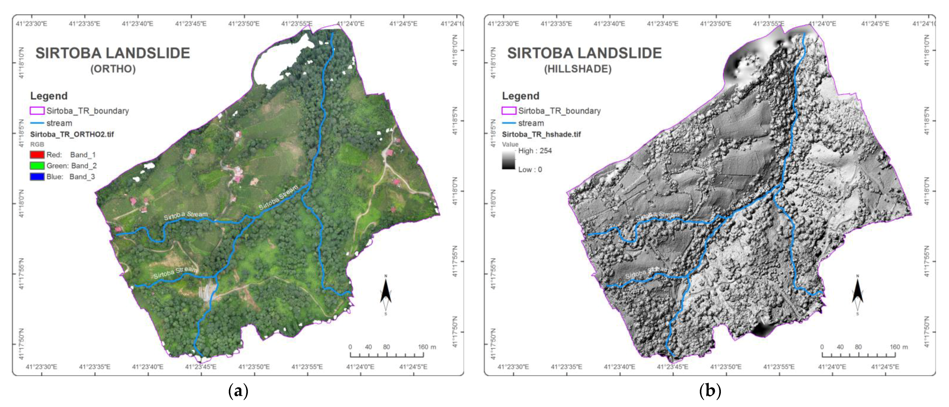
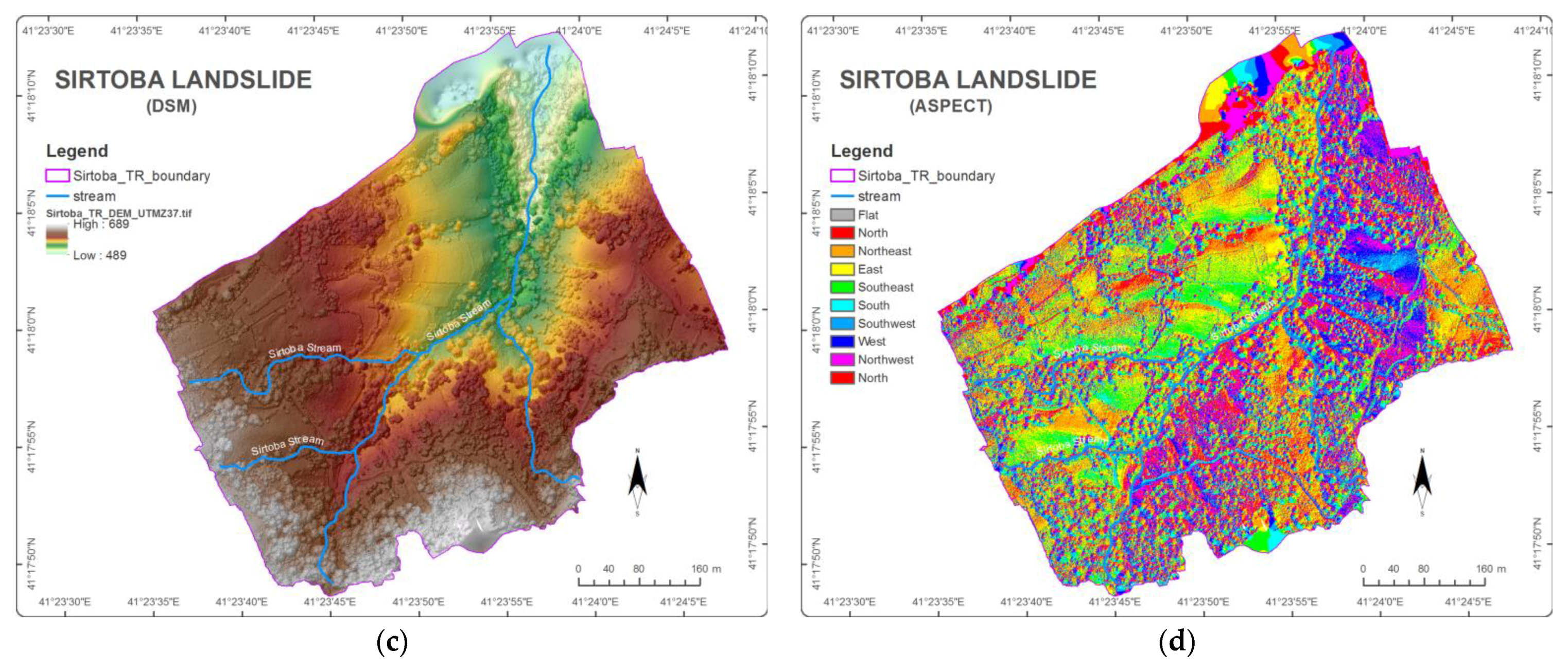
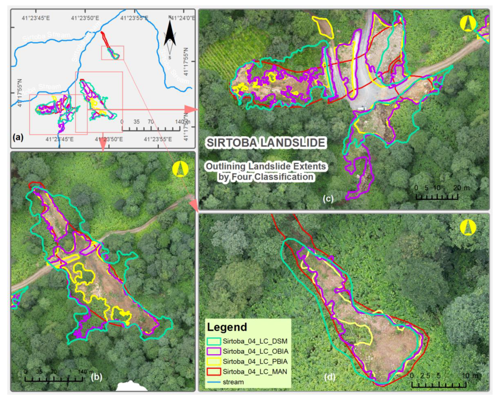
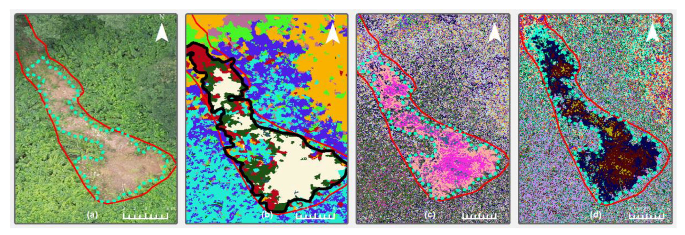
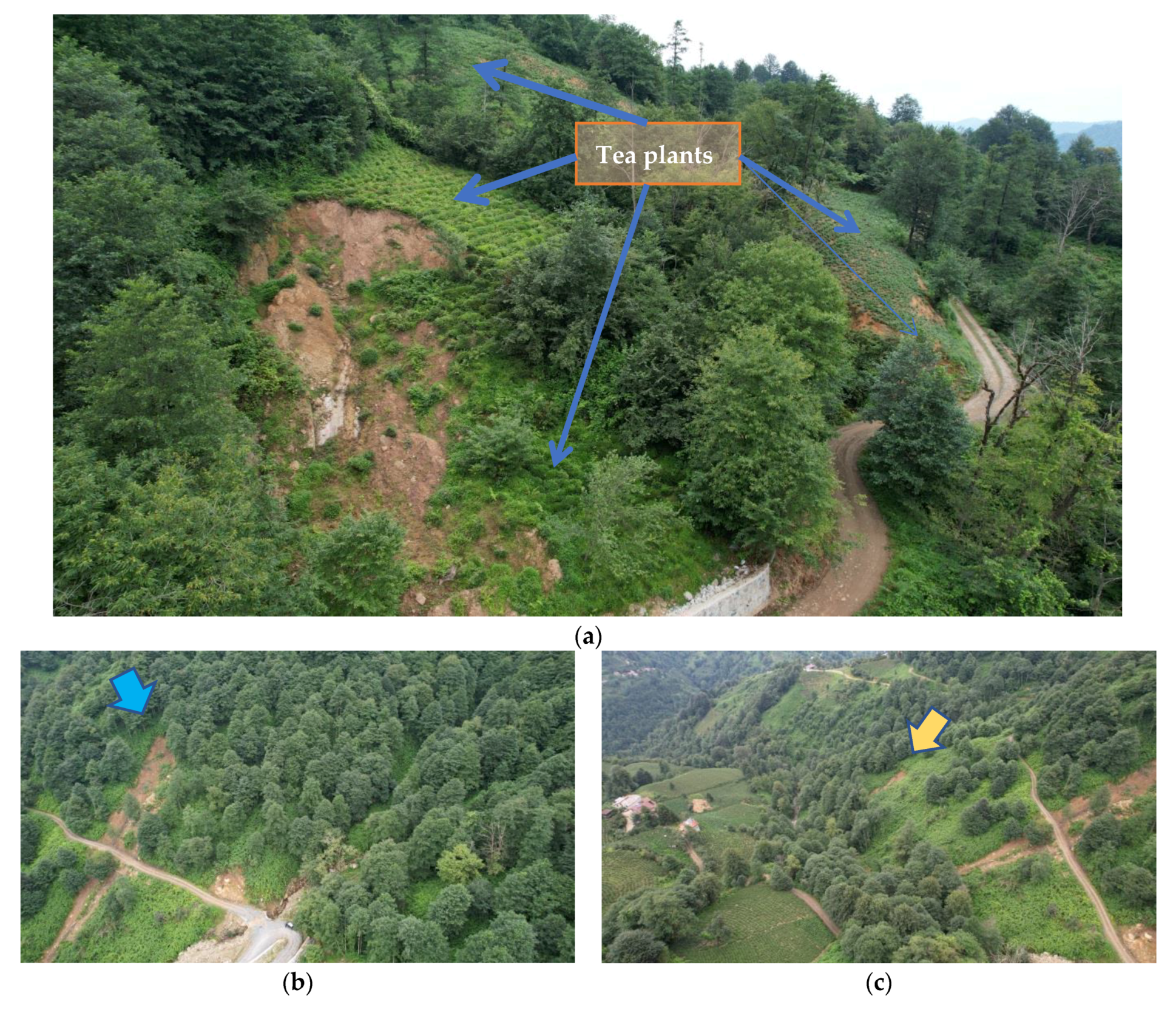
2.1.3. The Sirtoba Landslide Site of the Arhavi River Watershed (TURKEY)

The case study area of the Sirtoba landslide site is located southeast of Sirtoba Village in the Arhavi River Watershed, Arhavi Province, Turkey, at latitudes between 41.2967° and 41.3034°N and longitudes between 41.3932° and 41.4022°E in the WGS84 geographical coordinate system (Figure 4). The pilot area is 31.83 ha in size. The terrain has a very steep slope, with elevations ranging from 489 to 689 m above sea level. The distinctive typographic elevation differences reveal a variety of floristic habitat compositions. The forested lands include Anatolian chestnut (Cestanea sativa Mill.), bearded alder (Alnus glutinosa subsp. barbata (C.A. Mey. Yalt.), Oriental beech (Fagus orientalis Lipsky.), Oriental spruce (Picea orientalis L.), hornbeam (Carpinus orientalis), Scots pine (Pinus sylvestris L.), and sycamore (Platanus orientalis) trees. The main crop species in the agricultural areas are tea (Camellia sinensis L. Kuntz.), pears (Pyrus sp.), hazelnuts (Corylus avellana L.), kiwis (Actinidia sp.), apples (Malus sp.), and grapes (Vitis vinifera L.). The total area of the case study site is made up of 46.1% forest, 53.3% grassland and agricultural land, and 0.6% residential areas [87]. The geology of the research site consists of volcanic agglomerates and sedimentary rocks belonging to the geological Rhodope-Pontid Fragment. The geologic formations date from the Late Cretaceous Period to Quaternary limestone deposits [88]. Ultisol, inseptisol, and podzol soils are the predominant soil types in the region. The region experiences a climate that is typical of the Black Sea, which is very humid and heavily influenced by air masses carried by the sea. Data from the Arhavi Weather Station for 33 years (1985–2018) show that the mean annual temperature is 13.6 °C, with July being the hottest month (22.1 °C) and January being the coldest (6.5 °C) [89].
The landslides in the case study were triggered by heavy rainfall (136 mm in six hours) on 22 July 2021. The rain fell at a rate of 61 mm during the first hour of the rain event [89]. Within the study area, three major and one minor landslide with lengths of 117, 88, 75, and 23 m and widths of 33, 29, 13, and 15 m occurred during this event. The landslides were initiated as translational slides and then became debris avalanches [3] with liquefiable material’s cohesion loss due to undrained loading simultaneously after the extreme rainfall. The one in the tea garden remained a translational slide and accumulated as a colluvial mass near the road–stream junction. The landslides ranged in depth from 2 to 5 m. The flows ended up in Sirtoba Stream and then were washed away by rainwater. While allowing the clogged road to be used, some sediments on the deposited area were formed. Because of the steep slope, the landslides did not deposit sediments in a cone. Rather, the sediments ended up in streams and washed away.

2.2. Hardware, Software, and Methodology

2.2.1. UAV Flight Planning and Acquisition of UAV Imagery

In order to monitor and map the streamside landslides, high-tech UAVs were utilized, alongside photogrammetric software, to produce high-resolution (RGB) orthophoto maps, while sophisticated mapping was performed in GIS analysis software. The UAVs that we used were the DJI Mavic 2 Pro (in Greece), the DJI Mavic Mini 2 (in Romania), the DJI Matrice 300 RTK, and the DJI Air2S (in Turkey). The DJI Mini 2 has a 1/2.3” CMOS (complementary metal–oxide–semiconductor) sensor with a 12MP camera. The DJI Matrice 300 RTK (M300) has an integrated H20T camera system housing a 12-megapixel (MP) red, green, and blue (RGB) wide-angle camera with a focal length of 8 mm, a 20 MP zoom camera with 23× hybrid optical zoom capabilities, a 640 × 512 pixel radiometric thermal camera, and a 1200 m laser rangefinder. A Hasselblad L1D-20c camera with a 20 MP 1” CMOS sensor is included with the DJI Mavic 2. The DJI Air2S has a one-inch 20 MP CMOS sensor with a 22 mm equivalent lens [90]. Because of its size, the M300 was used for mapping streamside slopes in windy conditions, and the Air2S was used for mapping streams at a height of 2-3 m above water level. Then, the acquired images from M300 were used for orthomosaicking and DSM generation. The imagery taken by the Air2S was also used to delineate the stream network under the shading trees. Noontime (around 11:00–14:00) was selected for taking UAV images to reduce shadow effects. Although the period when the leaves fall is considered the best, allowing visibility under the canopy in forested riparian zones, in this study, the period with leaves was chosen in order to assess whether streamside landslides are able to be captured and delineated in such vegetated conditions. The flight altitude was set to 100, 150, and 124 m for Lefkothea, Chirlesti, and Sirtoba, respectively, in order to obtain uniform ground coverage for each flight (Table 1). Flight was avoided on windy days (>10 m/s). To ensure a 2–3 cm ground sampling distance (GSD), flight planning was set to obtain 80 percent overlap and 70 percent side-lap by using the polygon 2D mapping flight plan option. The flights were conducted on 1 July 2021 in Romania, on 1 September 2022 in Greece, and on 13 August 2022 in Turkey (Table 1). A single UAV image’s footprint on the ground was 141 × 94 m for Lefkothea in Greece, 69 × 52 m for Chirlesti in Romania, and 304 × 228 m for the Sirtoba site in Turkey.

2.2.2. Topographic Correction of Aerial Products

Data from GPS-GNSS (Global Positioning System/Global Navigation Satellite System) are essential for the image georeferencing process and provide highly accurate horizontal and vertical positioning for UAV products [91] in WGS84 geographical coordinates. Obtaining high accuracy in the finished products requires a density of 1 GCP/200 m2 [92]. The GPS-GNSS JAVAD TRIUMPH-1 receiver (San Jose, CA, USA) was used to include six (6) physical spots as GCPs for the Greek site (Table 1). The geospatial accuracy of the orthoimagery, rated at an XY RMSE of 0.1353 m and Z RMSE (DSM) of 0.9639 m accuracy, was ensured using the 6 GCPs. The GCPs for the Chirlesti mudflow site in Romania were captured with a Leica TCA1103 total station with 4 GCPs (Table 1). The XY RMSE for orthophotos was 0.1498 m, and the Z RMSE for the DSM product was 0.7985 m (Table 2). There was no GPS base station to be used to correct signals for data gathered by the GPS receivers in the Chirlesti and Lefkothea sites. Real-Time Kinematic (RTK) technology [93] provided high-precision image georeferencing in the Turkish case study. Before the flight plan, the satellite navigation geodetic system’s “base station” was installed. The DJI Matrice 300 RTK’s GNSS antenna served as a “rover.” Using a radio-telemetry system, the RTK system enabled the continuous transmission of GNSS corrections to the UAV, ensuring the real-time recording of the coordinates with an XY RMSE of 0.0768 m (orthophoto) and a Z RMSE (DSM) of 0.9813 m accuracy in the flight controller’s memory (Table 2) [94]. We did not need to employ coordinate post-processing kinematic (PPK) technology, which would have required more time because the survey sites were small [95].

2.2.3. Photogrammetric Workflow

The Pix4DMapper software package (Lausanne, Switzerland) was selected to generate the orthomosaic and digital surface model (DSM) of each case study site. Pix4DMapper is powerful well-established commercial Structure-from-Motion (SfM) software used worldwide [96]. With the aid of SfM technology, which is based on computer vision, photogrammetric reconstruction can be performed solely from RGB images, and using overlapping images, 3D information can be calculated without the need for prior knowledge of the camera’s surveyed reference points, calibration, or location and orientation in the scene [97,98,99]. The raw images were carefully inspected for any unwanted blurry images before any photometric processing. The UAV’s GPS data and IMU parameters were used to externally and internally orient the high-resolution imagery taken. The raw images were automatically tied to points to obtain the initial aerotriangulation [100]. In order to reduce the processing time, the intensity of the dense cloud was set to medium. Limits for the key and tie points were set at 40,000 and 4000, respectively. An adaptive camera fitting model was used for image matching. Then, dense point clouds were generated, followed by the mesh model and the texture. All of the parameters were set to medium for this workflow. The DSM was generated using the dense cloud points with Z RMSEs of 0.9639, 0.7985, and 0.9813 m for the Lefkothea, Chirlesti, and Sirtoba study sites, respectively (Table 2). Using the DSM and texture, the orthomosaic of each stream segment was generated at 2.56, 3.08, and 3.84 cm spatial resolution for each study site (Table 1). Furthermore, hillshade and aspect maps, based on the DSM as input, were generated in the spatial analysis toolbox in ArcGIS 10.6. Figure 5, Figure 6 and Figure 7 depict the orthomosaic, DSM, hillshade, and aspect maps for each site, respectively (Lefkothea in Greece, Chirlesti in Romania, and Sirtoba in Turkey).

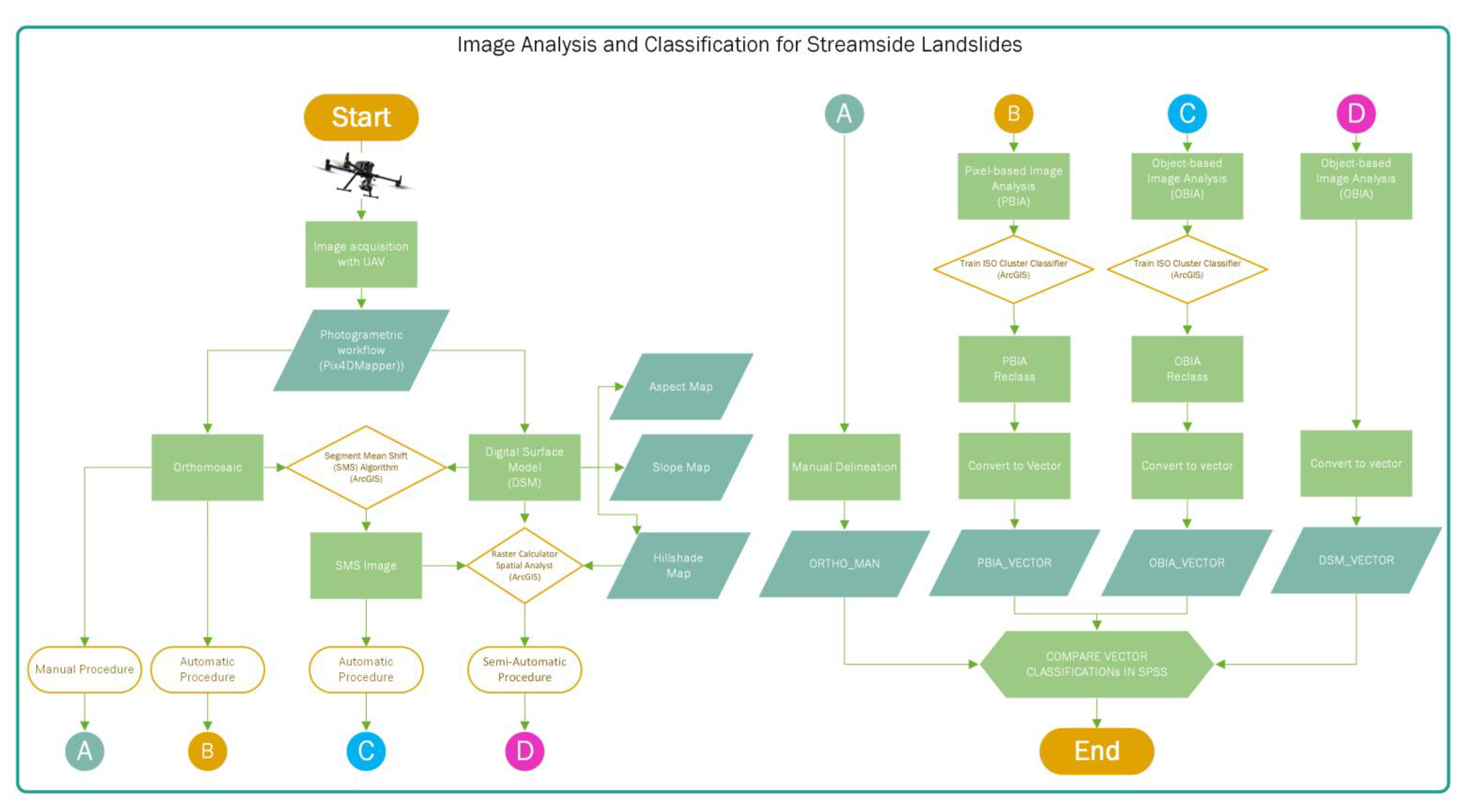
2.2.4. Image Analysis and Classification

Initially, manual delineation was performed in ArcGIS 10.6 (Redlands, CA, USA) in order to compare the results produced by the manual and automatic procedures. The combination of the above datasets was critical in order to identify the affected areas even in shadowed areas. The only limitation recorded was in areas covered by recent vegetation. The manual delineation of landslide deposits is the most common approach in the remote sensing community [101]. During this procedure, an experienced operator (an expertly trained geologist) identified the landslides by zooming and panning the three orthophotos and delineating the polygon boundaries, while a second experienced operator confirmed the uncertain boundaries (expertise in remote sensing photogrammetry). The orthomosaic’s bands, DSM, slope, and hillshade layers, which were derived from the DSM, were utilized as background datasets in order to map the boundaries of the landslides. The DSM data were also used to investigate the landslide depths in each study site. This was accomplished by evaluating the landslide cross-sectional profiles.
The ArcGIS “Segment Mean Shift” (SMS) tool under the Segmentation and Classification toolbox was utilized in order to extract streamside severe erosion and landslide events at each study site. The input layers used in this SMS analysis were the orthomosaic’s red, green, and blue bands, DSM, slope, and hillshade layers. Equal weighting was applied to each input layer, regardless of the units that were used in each layer [102]. The initial values were set to a spatial detail of 15, a spectral detail of 15.5, and a minimum segment size in pixels of 20. These values were selected in order to automatically identify feature objects/segments in the orthomosaic of each case study by grouping adjacent pixels together that have similar spectral and spatial characteristics. To make classification simple, the segmentation method eliminates the speckles and groups small pixels into substantial continuous areas.
The next process included the PBIA methods to automatically map the streamside landslides. The traditional PBIA approach assigns a land use/land cover class to a pixel that has the same size and shape [103]. We used ArcGIS’s “Train ISO (iterative self-organizing) Cluster Classifier” tool under the Segmentation and Classification toolbox [104] to classify land cover types, including landslides within each streamside (Figure 8). The orthomosaic dataset was utilized to perform automatic classification for the PBIA method. The spectral bands (RGB) of orthomosaic images for each site were chosen as input bands for PBIA processes using the ISO Cluster classifier. The maximum number of classes was set to 15, with a maximum number of iterations of 20. The maximum number of cluster merges per iteration was set to 5, and the maximum merge distance was set to 0.5. The minimum number of samples per cluster was set to 20 with a skip factor of 10. There were no additional raster files included in the process. The output classifier definition files were generated for the pixel-based image analysis and the object-based image analysis. The PBIA uses the objects’ spectral (band) characteristics [105] to classify land cover types. In the Sirtoba landslide–Arhavi River pilot area, the land cover types were divided into forests, tea gardens, hazelnut gardens, shrubs, and pastures. For the Chirlesti mudflow–Buzau River Watershed and Lefkothea–Aggitis River Watershed, the land cover types were divided into forested areas, agricultural land, urban development, and pasture lands. The spatial variation in various land covers in high-resolution images is not taken into account by pixel-based techniques used for moderate- and low-resolution imagery [106]. Instead, these techniques ignore nearby pixels that are a part of the same land cover. The pixel itself does not hold any neighboring or surrounding concept of an object. On the other hand, the OBIA method divides an image into segments by accumulating small pixels into vector objects [107,108]. These objects vary in size and shape. Because they are vector objects, there is no need for a vectorization process. Using their spectral, geometrical, and spatial properties (geometry, area, color, shape, texture, adjacency, etc.), these vectors can be used to classify images into any land cover class. Since the weighted OBIA analysis can be performed on any GIS layer, it gives users unlimited analysis options to choose from. For a thorough review of OBIA methods on remote sensing applications, an extensive review with references can be found in [107].
The ArcGIS software has been incorporated into OBIA algorithms for segment mean shift (SMS) and classification (SVM classifiers, random forest, Maximum Likelihood, and ISO Cluster) [102]. Then, the segmented images (SMS products) were classified by using ISO Cluster Unsupervised Image Classification. This tool enables automatic classification based on statistical variances in the spectral properties of the pixels (the computer determines which classes are present in the image). In each segmented image that resulted, 15 classes were selected as a threshold value, with a sample interval of 10 and a minimum class size of 20. These numbers were selected after several trials as the best option for separating the different colors representing distinct features in the images.
When the population standard deviation is unknown, Student’s t-test analysis can be used as a statistical method for evaluating assumptions about the mean of a small sample drawn from a normally distributed population [109]. Since we have only four classifications for each case study site, Student’s t-test analysis was employed to determine whether there were any statistical variations among the classifications. All statistical analyses were performed using IBM’s SPSS 19 Statistical software (IBM Corp., Armonk, NY, USA) for each study site.

3. Results

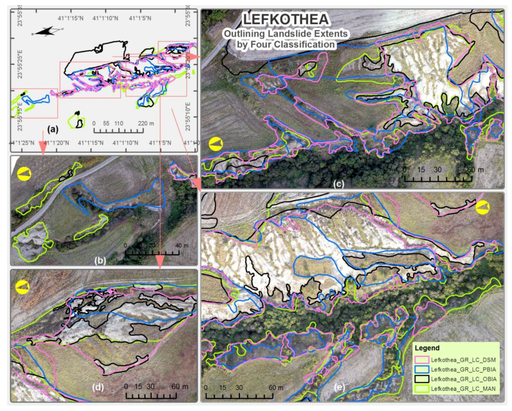
3.1. The Results of the Lefkothea Site

The results of manual delineation from orthomosaic imagery for the Lefkothea site in Greece are depicted in Figure 9a. The areas were categorized into 15 different classes. The areas of interest (landslide) belonged to categories 13, 14, and 15. By using merging operations during the classification stage, image objects from the same classes were combined to accurately represent the shape of the landslides. After the segments were created during the segmentation process, the second classification stage was applied to the SMS dataset to separate classes (Figure 9b). After the development of the PBIA-based and OBIA-based landslide models (Figure 9c,d), it is evident that there are differences among the four methodologies, as shown in Table 3. The majority of the landslides are located in the southeast, northwest, and west (Figure 10).
The SMS algorithm overestimated the affected areas, including agricultural fields that had a similar color to almost-flat areas. The specific dataset produced similar uncertainties to the ISO Cluster. The results showed that the manual classification based on the length of the landslide site was underestimated by the DSM and ISO Cluster algorithms and overestimated for the area of the Lefkothea site (Table 1). The test results showed that there was a statistical significance (p < 0.05) among the four classifications for the Lefkothea study site.
For the intersected areas, 50% of the OBIA classification area was covered by manual delineation, followed by 25% for PBIA and 16% for SMS classifications (Table 3). The same pattern was followed by the intersected perimeters at 22%, 12%, and 10% for OBIA, PBIA, and SMS classifications, respectively.

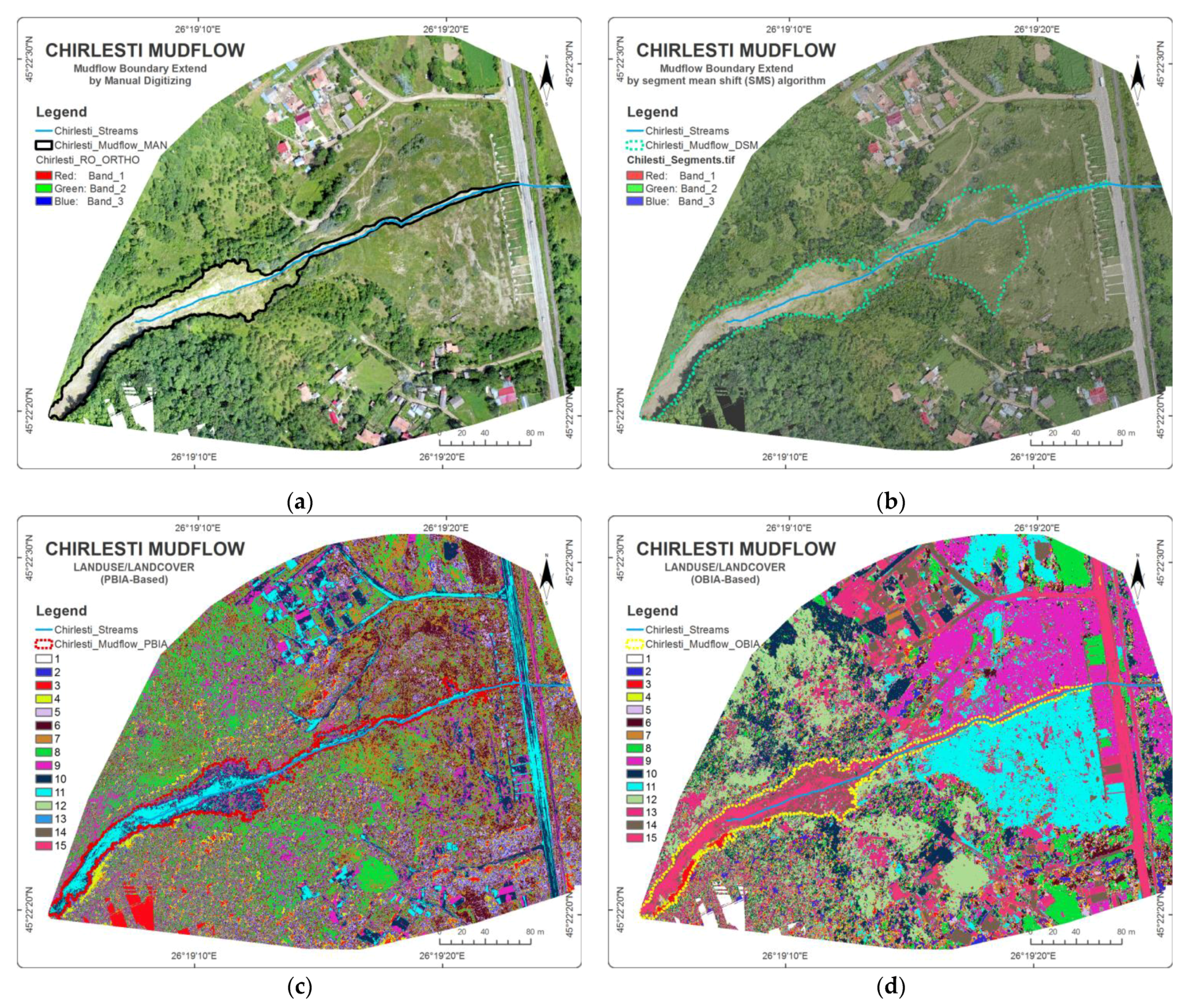
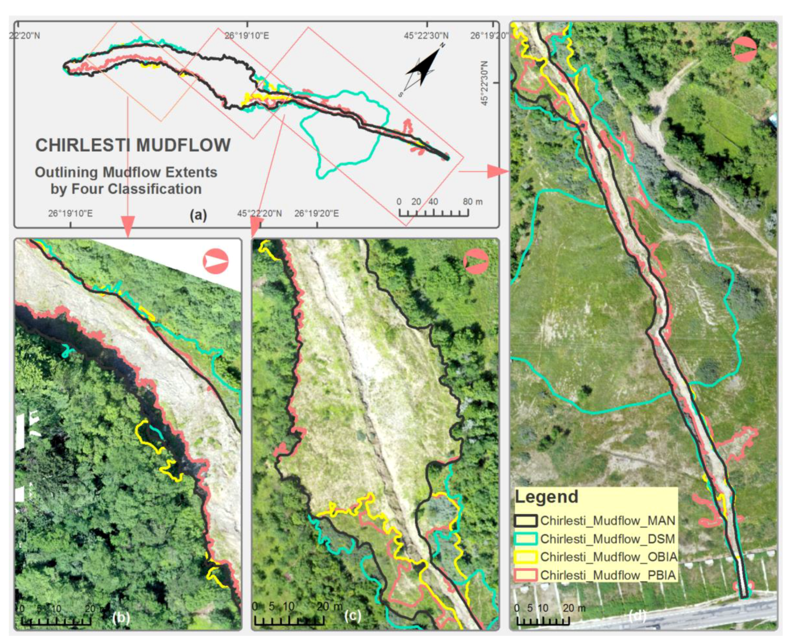
3.2. The Results of the Chirlesti Site

The ISO Cluster classifier used orthomosaic and segmented images for the Chirlesti mudflow site as input rasters. The maximum number of classes was limited to 15, with a maximum of 20 iterations. In each iteration, the maximum number of clusters to merge was set at 5, with a maximum merge distance of 0.5. With a skip factor of 10, the minimum number of samples per cluster was set at 20. The output classifier definition files for pixel-based image analysis and object-based image analysis were created. The output maps for the Chirlesti site in Romania are depicted in Figure 11. There are differences among the four methodologies in both events that are presented in Table 4. The segmentation parameters applied to the Chirlesti site were the same as those applied to the Greek Lefkothea site. The ISO Cluster algorithm underwent the same procedures. The results showed that the manual classification based on the orthoimage was underestimated by the DSM and ISO Cluster algorithms for the perimeter and the area of the Chirlesti mudflow site (Figure 12). The area of the mudflow site was underestimated by 8% by pixel-based ISO Cluster algorithms (Table 4). For the Chirlesti mudflow study site, Student’s t-test analysis revealed a statistical significance (p < 0.05) among the four classifications in both the perimeter and area. Because degraded and deposited areas may be better seen in DSM images than in the orthoimage (Figure 6c and Figure 12), the DSM-based classification of the mudflow site differed from the manual digitization by 91% (Table 4).
For the intersected areas, 5% of the OBIA classification area was covered by manual delineation, followed by 9% for PBIA and 48% for SMS classifications (Table 4). The intersected perimeters were 5%, 18%, and 18% for OBIA, PBIA, and SMS classifications, respectively (Table 4).

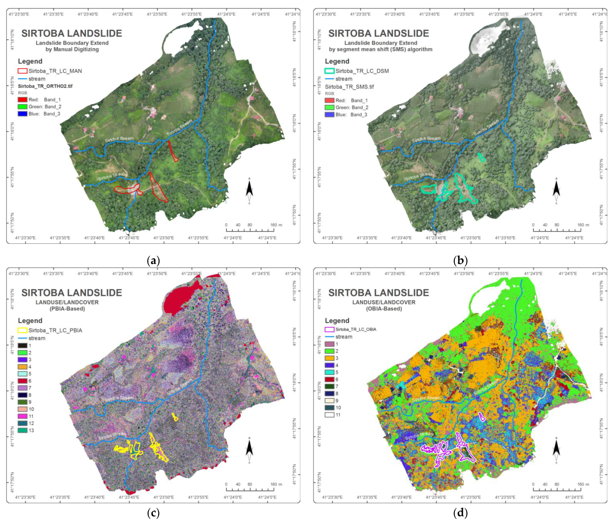
3.3. The Results of the Sirtoba Site

The ad hoc and final segmentation parameters used at the Sirtoba site were the same as those used at the Chirlesti mudflow site in Romania and the Lefkothea site in Greece. In addition to the ISO Cluster classification technique used for the other two sites, the region-grouping algorithm was used to fine-tune the classification for the Sirtoba site in Turkey. The classification outputs for the Sirtoba site are captured in Figure 13. For the ortho-based image analysis, the automatic unsupervised classification technique produced 13 classes (Figure 13c), and for segment-mean-shift-based image analysis, it produced 11 classes (Figure 13d). To remove speckles caused by plants within the landslides, classes 11, 12, and 13 were merged. In a similar manner, classes 9, 10, and 11 were combined for the OBIA-based classification. Similar disparities existing between the four approaches for the two situations are also noted in Table 5. The results showed that the manual classification based on the orthoimage was underestimated by the DSM and ISO Cluster algorithms for the perimeter of the Sirtoba Landslides (Figure 14). On the other hand, the landslide area was overestimated by pixel-based ISO Cluster algorithms by 27% (Table 5). According to Student’s t-test analysis, the four classifications for the Sirtoba Landslide research site have a statistical significance (p < 0.05) in terms of both the perimeter and area. Figure 7d depicts the locations of the landslides, which occurred on the terrain facing north, northeast, and east. A detailed view of the landslide boundary extent determined by the four distinct classifications in the orthophoto image can be seen in Figure 14. Field observations revealed that the soil in these regions is almost always moist. Following a significant downpour, these places are excessively susceptible to landslides.
For the intersected areas, 26% of the OBIA classification area was covered by manual delineation, followed by 19% for PBIA and 40% for SMS classifications (Table 5). The same pattern was followed by the intersected perimeters at 27%, 14%, and 33% for OBIA, PBIA, and SMS classifications, respectively (Table 5).

4. Discussion

Given the variety of shapes and sizes that landslides can take, detecting landslides is still a difficult task. Due to tree shadows, automatic classifications underestimated the extent of the landslide boundaries, particularly at the Chirlesti mudflow site in Romania. The riparian vegetation along the streams has covered transported sediments, which were only discovered in situ at the Lefkothea site in Greece and the Sirtoba site in Turkey. The main triggering factor for the landslide in each study area was extreme rainfall. This is true for most of the studies we cited in the Introduction section [4,5,12,88]. For instance, the Sirtoba site in Turkey received 160 mm of precipitation within a 6 hr period during the rainfall event on July 22, 2021. In order to see the variation in the runoff volume for each vegetation type in the Sirtoba site, we installed surficial erosion runoff plots. Through these runoff plots, we collected and measured the runoff water on the forested lands, tea garden fields, hazelnut garden fields, and grasslands of the Arhavi River Watershed, where the Sirtoba landslide site is located. The preliminary data from December 2021 to December 2022 showed that the runoff volumes were 0.9 L/day for forested lands, 1.3 L/day for tea gardens, 6.7 L/day for grasslands, and 15 L/day for hazelnut gardens. This demonstrated that trees and tea plants regulate the surficial runoff water. It was also observed that in the case of any extreme rain events, the leaves and roots of tea plants let the excess water infiltrate into the soil rapidly, causing saturation and triggering landslides.
Another triggering factor was the steep slopes of the study sites. Through their root systems, the extensive tree canopy was expected to preserve the soil and prevent landslides. This was not the case on very steeply sloped terrains [110]. As a result, the Sirtoba site saw numerous landslides during a single heavy rainfall event. The shallow soil depth and the shale layer forming the bedrock contributed to triggering the landslides. This specific study focused on streamside landslides, which differ from other landforms, as they occur in and are connected to the stream network and, in most cases, are generated by the force of water in vulnerable soils under high slopes [111]. The soil moisture content on the northern aspects (north, northeast, and northwest) is more than that on other aspects [112,113,114,115]. This makes the soil on the northern aspects more saturated than on other aspects. Furthermore, it increases the probability of a landslide. The authors of [116] had similar findings in their study, which they conducted on hillslopes in the Black Soil (Mollisols) Area of Northeast China.
The depth of the topsoil varies between 1 and 6 m at the Sirtoba landslide site in Turkey. A shale layer begins underneath the topsoil. Due to heavy downpours in the study area, trees in the forested lands and tea plants in the tea garden slow the runoff water and let it drain into the soil. The shale beneath forested lands and tea gardens collects drained water as a thin layer between the upper soil layer and the shale, causing the upper soil layer to move downward. At the Chirlesti site in Romania, the same shale formation existed along the mudflow. After the extreme rainfall at the two study sites, we believe that the shallow shale formation is the second contributing factor.
Landslide mapping via OBIA and PBIA methods has been applied previously, e.g., in Hokkaido province of Japan, by also using DEMs and vegetation indices (e.g., NDVI) to detect changes between satellite images taken on different dates and by comparing the vegetation and elevation products [117]. The NDVI index is a worldwide known vegetation index that can be used in dense vegetated areas to spot and classify landslides [118]. The specific index was utilized in a previous step by using free satellite images in order to highlight the places of interest (not presented here), which were further investigated with the current UAV flights in greater resolution.
The UAVs used were not equipped with a near-infrared camera to acquire the NDVI index. In addition, a full-scale object-level change detection method (segmentation and classification) has been used effectively and efficiently for change detection and the extraction of artificial objects with rich structure information from multiple images of the Wenchuan Earthquake area affected by landslides [119]. Generally, semi-automatic or fully automatic UAV-based photogrammetry has been utilized to detect longitudinal and transverse cracks (e.g., on the road or the railway network) and assess their severity in landslide areas [95,120,121]. These models (OBIA and PBIA) underwent testing at the chosen landslide locations in Greece, Romania, and Turkey. The models offered different results for each of the three areas, per the accuracy assessment findings. This difference was primarily caused by the fact that many landslide bodies were hidden by vegetation and shadowy areas. In order to minimize these effects, the classified images were aggregated by using an 8x8-cell region-grouping algorithm under the Spatial Analyst Tool in ArcGIS 10.6. Additionally, some landslides were cut by the forested road network in the Turkish site (Sirtoba). During the landslide events, all roads within the affected area were moved downward. These roads were reconstructed, and the supporting walls were built to prevent upper slope mass movements. The final result was different (fewer classes produced in some of the case studies) due to the colors contained in each orthomosaic. All of these factors affected the accurate size of the area produced in each method. For all case studies, the OBIA model provided the best results, with values that were closer to those obtained by manual delineation (only a 2% difference in area size).
Temporal variation in vegetational growth is one of the limitations in identifying and delineating the extent of landslides [66,76]. It is much easier to identify the landslide’s boundary immediately following the landslide event using UAVs and sediment and mud deposits on vegetation. In Turkey’s Sirtoba site, the vegetation covered the affected area within a month (Figure 15a). The ability of the vegetation to cover the landslide area at the Lefkothea site in Greece and the Chirlesti site in Romania, on the other hand, took longer than at the Sirtoba site in Turkey. This is one of the reasons why the perimeter/area ratio at the Sirtoba site is higher than at the Lefkothea and Chirlesti sites (Table 3, Table 4 and Table 5).
Using the Minimum Bounding Geometry Toolbox in ArcGIS, the width and length of each landslide in the case study areas were estimated. For comparison, the average values for each classification type were subtracted from the manual classification results (Table 6). According to the findings depicted in Table 6, the Lefkothea and Sirtoba sites’ average widths varied for each approach. Surprisingly, all methods except the one that used DSM data to obtain results indicated the same width at the Chirlesti mudflow site. This might be attributable to a DSM image’s roughness property, which can more accurately depict the eroded and deposited areas than other techniques [59,60,122]. Table 6 shows the W/L ratio results for the four different classifications in each study site. Three out of four classifications showed an average W/L ratio of 0.450 at Sirtoba in Turkey. Small width/length ratios are indicators of thin-shaped landslides that have a typical mix of translational debris slides and debris avalanches on steep slopes. The W/L ratio for manual delineation at the Sirtoba site was lower than in other classifications because the landslides reached streams through the trees. Because of the tree cover, the ISO Cluster classification and SMS algorithms failed to detect those routes. The detection of those landslides was possible with manual delineation and in situ observations. The Chirlesti site followed the same thin-shaped mudflow and had the longest landslide among the three study sites. The W/L ratio was higher in the segmented classification than in the other classifications. It showed a wide (elongated) mudflow pattern. With the help of the DSM and hillshade images, the cone (deposited area) was clearly visible and distinguishable from its surroundings (Figure 6c and Figure 12d). The Chirlesti mudflow site is a continuous phenomenon that started in 1953 [82]. The detailed shape and characteristics of the mudflow can be found in Lahousse et al. [82]. The W/L values were similar for all classifications at the Lefkothea site. They were higher than the W/L values at the Chirlesti site, but lower than those at the Sirtoba site.
The positional accuracies of GPS data embedded within each UAV image and the GCPs used to create orthophotos and DSMs might slightly affect the areas and lengths determined using the four classifications. This can be attributed to the nature of GPS signal errors introduced by atmospheric delays (ionospheric effects), space weather, ephemeris effects, and so on [93,123]. In normal conditions, GPS signals have 3–15 m positional errors in XY and 10–20 m in the Z-direction when GPS satellites’ selective availability (SA) feature is turned off (an intentional degradation of public GPS signals). With the survey-grade GPS receivers we used in the Lefkothea and Chirlesti study sites, we were able to reduce these Z-directional errors to close to one meter and the XY-directional errors to less than 15 cm. Even with the help of real-time kinematic processing (RTK, CORS, or WAAS), these errors can be reduced to centimeter accuracy [31,93]. In the Chirlesti, Lefkothea, and Sirtoba sites, the UAV images were taken at an oblique angle. Therefore, even with differential GPS data applied, the off-nadir images might be linked to the Z errors introduced in our DSM products [79,82,124]. This was the reason why our Z errors in orientation in GCPs were close to 1 m. Agüera-Vega et al. [124] reported that DSM positional errors were mostly affected by the UAV’s flight altitude and the number of GCPs rather than the terrain morphology. They found no statistical significance among the XY RMSE, flight altitude, or terrain morphology. They used the same number of GCPs as we did in our study.
The spatial intersections (overlaps) of the classification with manual delineation varied at each study site. The largest area of agreement between manual and OBIA classifications was 50% for Lefkothea, 26% for Sirtoba, and 5% for the Chirlesti site. The SMS and manual classification agreement at intersected areas were 48% for Chirlesti, 40% for Sirtoba, and 16% for the Chirlesti study site. At the Lefkothea site, there was a 25% intersection between manual and PBIA classifications. It was 19% for Sirtoba and 9% for the Chirlesti site (Table 3, Table 4 and Table 5). There was no relation between the W/L ratio and intersected areas either. One could have expected that the percent difference in area and the percent intersected area would add up to 100 percent. This was not the case for these study sites. This could be explained by stating that spatial intersections and non-spatial area differencing are not the same and cannot be comparable.

5. Conclusions

In the context of this study, manual landslide delineation, a segmentation process, and two mapping models (OBIA and PBIA) were created based on the characteristics of each selected landslide. The case studies under analysis have had significant impacts on the affected areas, which have been altered as a result, including urban settings, forested areas, and agricultural fields (Figure 16, Figure 17 and Figure 18). The comparison highlighted differences among the various methodologies on the affected areas and perimeters. Among the four classifications, the OBIA produced the best intersection across all study sites (area-wise, 2% deviation from the control points). The classification model with the lowest performance was the PBIA. The only classification that was able to detect the debris fan at the Chirlesti mudflow site was the SMS classification using the hillshade image. The results indicated that the terrain (slope), the aspect of the slope, the shape of the landslide, the vegetation cover, and the soil/parent material are highly implicated in the landslide phenomena and their future evolution. The creation of preventative streamside landslide buffers will aid in mitigating the effects of similar streamside events in the Black Sea and the Mediterranean, as well as those in areas already mentioned above [125]. The best ways to prevent or reduce adverse effects on both the urban environment and the natural environment are to combine gray-green adaptation, preventive, and mitigation methods (a combination of targeted nature-based solutions with appropriate engineering techniques) [126,127]. Furthermore, knowledge about the subsurface properties would help to define the spatial occurrence and extent of the landslides [128]. As for future directions, frequent three-dimensional monitoring via UAV-based photogrammetry (including oblique imagery for the Z-axis) would enable us to calculate the volume of the transported material. This could be further achieved by also implementing field monitoring, including alert sensors to capture the events immediately (as in many cases, vegetation can cover previously unrecorded landslides).
Landslides are one of the major threats causing soil and ecosystem degradation and are considered of high importance for the European Union but also for the Black Sea Region [129]. The EU Thematic Strategy for Soil Protection calls “for actions and means for the protection and sustainable use of soils as a physical platform on which human activities are developed” [130,131]. The goal is to pinpoint areas at risk for landslides and other soil threats, set risk reduction objectives there, and create the necessary tasks, programs, and management plans of action [132]. In order to quantify the occurrence of landslides, it is necessary to have applicable data; for this reason, landslide inventories are of high importance [133]. Attention must be given when comparing spatial intersections with non-spatial area differencing. Inventories can be either prepared manually or can be semi-automatically developed in a GIS environment, or even available to everyone through a web-GIS platform [134]. Such a cloud-based GIS tool includes surface ruptures, main shocks, faults, aftershocks, earthquake-triggered landslides, and earthquake intensity from the 2008 Wenchuan Earthquake [135] in addition to other sources of hazard data. The proposed framework can support landslide experts, land managers, and responsible authorities by providing tested UAV-based methods and guidelines for mapping areas at risk of landslides, with an emphasis on streamside events. The proposed framework is a substantial development that can help identify landslides easily and quickly in order to create an inventory focused on the vulnerable Black Sea Region but also allow recommendations of targeted nature-based solutions for preventive measures. For further research, relationships among land properties, reliefs, forests, and climate extremes can be analyzed.

Author Contributions

Conceptualization, M.Y., P.K. and D.C.D.; methodology, M.Y., P.K., G.G. and D.C.D.; validation, M.Y., P.K., and D.C.D.; formal analysis, M.Y., P.K. and D.C.D.; investigation, M.Y., G.G., P.K. and D.C.D.; writing—original draft preparation, M.Y., P.K. and D.C.D.; writing—review and editing, G.N.Z., M.T. and M.M.; visualization, M.Y., G.G., P.K. and D.C.D.; supervision, G.N.Z.; project administration, G.N.Z., M.T. and M.M.; funding acquisition, G.N.Z., M.T. and M.M. All authors have read and agreed to the published version of the manuscript.

Funding

The current work was realized in frames of the Joint Operational Black Sea Programme 2014-2020, the Project BSB 963 “Protect-Streams-4-Sea”, with the financial assistance of the European Union. The content of this publication is the sole responsibility of the authors and in no case should be considered to reflect the views of the European Union.

Data Availability Statement

Not applicable.

Conflicts of Interest

The authors declare no conflict of interest. The funders had no role in the design of the study; in the collection, analyses, or interpretation of data; in the writing of the manuscript; or in the decision to publish the results.

Abbreviations

CORSContinuously Operating Reference Stations
CMOSComplementary Metal–Oxide–Semiconductor
DSMDigital Surface Model
GCPsGround Control Points
GISGeographic Information Systems
GNSSGlobal Navigation Satellite System
GPSGlobal Positioning System
DGPSDifferential GPS
GPS-GNSSGlobal Positioning System/Global Navigation Satellite System
GSDGround Sampling Distance
IMUInteractive Multimedia Unit
InSARInterferometric Synthetic Aperture Radar
ISOIterative Self-Organizing
LiDARLight Detection and Measurement
LisaLaser Interferometer Space Antenna
MLMachine Learning
MPMegapixel
NDSINormalized Difference Soil Index
NDVINormalized Difference Vegetation Index
NDWI Normalized Difference Water Index
NENortheast
OBIAObject-Based Image Analysis
OTDROptical Time Domain Reflectometer
PBIAPixel-Based Image Analysis
PPKPostprocessing Kinematic
RGBRed, Green, Blue
RTKReal-Time Kinematic
SARSynthetic Aperture Radar
SfMStructure from Motion
SMSSegment Mean Shift
SVMSupport Vector Machine
SWSouthwest
UAVUnmanned Aerial Vehicle
WAASWide Area Augmentation System
WGS84World Geodetic System 1984
WSNWireless Sensor Networks

References

  1. Mokarram, M.; Sathyamoorthy, D. A review of landform classification methods. Spat. Inf. Res. 2018, 26, 647–660. [Google Scholar] [CrossRef]
  2. Intrieri, E.; Gigli, G.; Casagli, N.; Nadim, F. Brief communication” Landslide Early Warning System: Toolbox and general concepts”. Nat. Hazards Earth Syst. Sci. 2013, 13, 85–90. [Google Scholar] [CrossRef]
  3. Hungr, O.; Leroueil, S.; Picarelli, L. The Varnes classification of landslide types, an update. Landslides 2014, 11, 167–194. [Google Scholar] [CrossRef]
  4. Scaioni, M.; Longoni, L.; Melillo, V.; Papini, M. Remote sensing for landslide investigations: An overview of recent achievements and perspectives. Remote Sens. 2014, 6, 9600–9652. [Google Scholar] [CrossRef]
  5. Schuster, R.L.; Wieczorek, G.F. Landslide triggers and types. In Landslides; Routledge: London, UK, 2018; pp. 59–78. [Google Scholar]
  6. Šilhán, K. Dendrogeomorphology of different landslide types: A review. Forests 2021, 12, 261. [Google Scholar] [CrossRef]
  7. Varnes, D.; Eckel, E. Landslide types and processes. In Landslides and Engineering Practice by the Committee on Landslide Investigations; National Research Council (U.S.), Highway Research Board Special Report; Committee on Landslide Investigations: Washington DC, USA, 1958. [Google Scholar]
  8. Bracken, L.J.; Turnbull, L.; Wainwright, J.; Bogaart, P. Sediment connectivity: A framework for understanding sediment transfer at multiple scales. Earth Surf. Process. Landf. 2015, 40, 177–188. [Google Scholar] [CrossRef]
  9. Campforts, B.; Shobe, C.M.; Steer, P.; Vanmaercke, M.; Lague, D.; Braun, J. HyLands 1.0: A hybrid landscape evolution model to simulate the impact of landslides and landslide-derived sediment on landscape evolution. Geosci. Model Dev. 2020, 13, 3863–3886. [Google Scholar] [CrossRef]
  10. Huang, Y.; Xu, C.; Zhang, X.; Li, L. Bibliometric analysis of landslide research based on the WOS database. Nat. Hazards Res. 2022, 2, 49–61. [Google Scholar] [CrossRef]
  11. Jasim, M.M.; Al-Khaddar, R.M.; Al-Rumaithi, A. Prediction of bearing capacity, angle of internal friction, cohesion, and plasticity index using ANN (Case Study of Baghdad, Iraq). Int. J. Civ. Eng. Technol. 2019, 10, 2670–2679. [Google Scholar]
  12. Deb, S.K.; El-Kadi, A.I. Susceptibility assessment of shallow landslides on Oahu, Hawaii, under extreme-rainfall events. Geomorphology 2009, 108, 219–233. [Google Scholar] [CrossRef]
  13. Zhang, H.; Zhao, Z.; Ma, G.; Sun, L. Quantitative evaluation of soil anti-erodibility in riverbank slope remediated with nature-based soil bioengineering in Liaohe River, Northeast China. Ecol. Eng. 2020, 151, 105840. [Google Scholar] [CrossRef]
  14. Schmidt, K.; Roering, J.; Stock, J.; Dietrich, W.; Montgomery, D.; Schaub, T. The variability of root cohesion as an influence on shallow landslide susceptibility in the Oregon Coast Range. Can. Geotech. J. 2001, 38, 995–1024. [Google Scholar] [CrossRef]
  15. EPA. Total Maximum Daily Load for Sediment Redwood Creek, California; United States Environmental Protection Agency Region, Ed.; Generic: San Francisco, CA, USA, 1998; p. 73. [Google Scholar]
  16. Sutherland, D.G.; Ball, M.H.; Hilton, S.J.; Lisle, T.E. Evolution of a landslide-induced sediment wave in the Navarro River, California. Geol. Soc. Am. Bull. 2002, 114, 1036–1048. [Google Scholar] [CrossRef]
  17. Benda, L.; Dunne, T. Stochastic forcing of sediment supply to channel networks from landsliding and debris flow. Water Resour. Res. 1997, 33, 2849–2863. [Google Scholar] [CrossRef]
  18. Schuster, R.L.; Highland, L.M. Impact of landslides and innovative landslide-mitigation measures on the natural environment. In Proceedings of the International Conference on Slope Engineering, Hong Kong, China, 8–10 December 2003. [Google Scholar]
  19. Benda, L. The influence of debris flows on channels and valley floors in the Oregon Coast Range, USA. Earth Surf. Process. Landf. 1990, 15, 457–466. [Google Scholar] [CrossRef]
  20. Swanson, F. Natural disturbance effects on riparian areas. In Riparian Resources, Proceedings of the Symposium on the Disturbances, Management, Economics, and Conflicts Associated with Riparian Ecosystems, Logan, Utah, 18–19 April 1991; Utah State University: Logan, UT, USA, 1994; pp. 11–14. [Google Scholar]
  21. Baum, R.L.; Reid, M.E. Geology, hydrology, and mechanics of a slow-moving. In Clay Shale Slope Instability; The Geological Society of America: Boulder, CO, USA, 1995; Volume 10, p. 79. [Google Scholar]
  22. Bogaard, T.A.; Greco, R. Landslide hydrology: From hydrology to pore pressure. Wiley Interdiscip. Rev. Water 2016, 3, 439–459. [Google Scholar] [CrossRef]
  23. Dikau, R.; Cavallin, A.; Jäger, S. Databases and GIS for landslide research in Europe. Geomorphology 1996, 15, 227–239. [Google Scholar] [CrossRef]
  24. Pánek, T. Recent progress in landslide dating: A global overview. Prog. Phys. Geogr. 2015, 39, 168–198. [Google Scholar] [CrossRef]
  25. Glade, T.; Crozier, M.J. Landslide hazard and risk: Concluding comment and perspectives. In Landslide Hazard Risk; Wiley: Chichester, UK, 2005; pp. 767–774. [Google Scholar]
  26. Rogers, D.; Tsirkunov, V. Costs and benefits of early warning systems. In Global Assessment Report; ISDR: Geneva, Switzerland; The World Bank: Washington, DC, USA, 2011. [Google Scholar]
  27. Pecoraro, G.; Calvello, M.; Piciullo, L. Monitoring strategies for local landslide early warning systems. Landslides 2019, 16, 213–231. [Google Scholar] [CrossRef]
  28. Xu, Q.; Peng, D.; Zhang, S.; Zhu, X.; He, C.; Qi, X.; Zhao, K.; Xiu, D.; Ju, N. Successful implementations of a real-time and intelligent early warning system for loess landslides on the Heifangtai terrace, China. Eng. Geol. 2020, 278, 105817. [Google Scholar] [CrossRef]
  29. Guzzetti, F.; Mondini, A.C.; Cardinali, M.; Fiorucci, F.; Santangelo, M.; Chang, K.-T. Landslide inventory maps: New tools for an old problem. Earth-Sci. Rev. 2012, 112, 42–66. [Google Scholar] [CrossRef]
  30. Azzam, R.; Arnhardt, C.; Fernandez-Steeger, T. Monitoring and early warning of slope instabilities and deformations by sensor fusion in self-organized wireless ad-hoc sensor networks. J. SE Asian Appl. Geol. 2010, 2, 163–169. [Google Scholar]
  31. Guo, J.; Yang, J.I.; Ding, Z.G.; Zhou, P.G.; Zhu, X.G. GPS landslide monitoring. J. Geod. Sci. 2004, 10, 65–70. [Google Scholar]
  32. Intrieri, E.; Gigli, G.; Mugnai, F.; Fanti, R.; Casagli, N. Design and implementation of a landslide early warning system. Eng. Geol. 2012, 147, 124–136. [Google Scholar] [CrossRef]
  33. Jeong, S.; Ko, J.; Kim, J. The effectiveness of a wireless sensor network system for landslide monitoring. IEEE Access 2019, 8, 8073–8086. [Google Scholar] [CrossRef]
  34. Li, J.; Wang, W.; Han, Z.; Li, Y.; Chen, G. Exploring the impact of multitemporal DEM data on the susceptibility mapping of landslides. Appl. Sci. 2020, 10, 2518. [Google Scholar] [CrossRef]
  35. Pardeshi, S.D.; Autade, S.E.; Pardeshi, S.S. Landslide hazard assessment: Recent trends and techniques. SpringerPlus 2013, 2, 523. [Google Scholar] [CrossRef]
  36. Baeza, C.; Lantada, N.; Amorim, S. Statistical and spatial analysis of landslide susceptibility maps with different classification systems. Environ. Earth Sci. 2016, 75, 1318. [Google Scholar] [CrossRef]
  37. Reichenbach, P.; Rossi, M.; Malamud, B.D.; Mihir, M.; Guzzetti, F. A review of statistically-based landslide susceptibility models. Earth-Sci. Rev. 2018, 180, 60–91. [Google Scholar] [CrossRef]
  38. Zaimes, G.Ν.; Tamparopoulos, A.E.; Tufekcioglu, M.; Schultz, R.C. Understanding stream bank erosion and deposition in Iowa, USA: A seven year study along streams in different regions with different riparian land-uses. J. Environ. Manag. 2021, 287, 112352. [Google Scholar] [CrossRef]
  39. Valjarević, A.; Algarni, S.; Morar, C.; Grama, V.; Stupariu, M.; Tiba, A.; Lukić, T. The coastal fog and ecological balance for plants in the Jizan region, Saudi Arabia. Saudi J. Biol. Sci. 2022, 30, 103494. [Google Scholar] [CrossRef] [PubMed]
  40. Jiang, Z.; Zhao, C.; Yan, M.; Wang, B.; Liu, X. The Early Identification and Spatio-Temporal Characteristics of Loess Landslides with SENTINEL-1A Datasets: A Case of Dingbian County, China. Remote Sens. 2022, 14, 6009. [Google Scholar] [CrossRef]
  41. Shahabi, H.; Hashim, M. Landslide susceptibility mapping using GIS-based statistical models and Remote sensing data in tropical environment. Sci. Rep. 2015, 5, 9899. [Google Scholar] [CrossRef]
  42. Álvarez López, Y.; García Fernández, M.; Grau, R.; Las-Heras, F. A synthetic aperture radar (SAR)-based technique for microwave imaging and material characterization. Electronics 2018, 7, 373. [Google Scholar] [CrossRef]
  43. Prokop, A.; Panholzer, H. Assessing the capability of terrestrial laser scanning for monitoring slow moving landslides. Nat. Hazards Earth Syst. Sci. 2009, 9, 1921–1928. [Google Scholar] [CrossRef]
  44. Chen, Z.; Zhang, B.; Han, Y.; Zuo, Z.; Zhang, X. Modeling accumulated volume of landslides using remote sensing and DTM data. Remote Sens. 2014, 6, 1514–1537. [Google Scholar] [CrossRef]
  45. Hu, H.; Fernandez-Steeger, T.M.; Dong, M.; Azzam, R. Landslide stability analysis on basis of Lidar data extraction. In Proceedings of the EGU General Assembly Conference 2010, Vienna, Austria, 2–7 May 2010; p. 652. [Google Scholar]
  46. Jaboyedoff, M.; Oppikofer, T.; Abellán, A.; Derron, M.-H.; Loye, A.; Metzger, R.; Pedrazzini, A. Use of LIDAR in landslide investigations: A review. Nat. Hazards 2012, 61, 5–28. [Google Scholar] [CrossRef]
  47. NASA; ESA. Laser Interferometer Space Antenna (LISA) Measurement Requirements Flowdown Guide; NAES Agengy, Ed.; NASA: Washington, DC, USA; ESA: Paris, France, 2011. [Google Scholar]
  48. Raspini, F.; Ciampalini, A.; Del Conte, S.; Lombardi, L.; Nocentini, M.; Gigli, G.; Ferretti, A.; Casagli, N. Exploitation of amplitude and phase of satellite SAR images for landslide mapping: The case of Montescaglioso (South Italy). Remote Sens. 2015, 7, 14576–14596. [Google Scholar] [CrossRef]
  49. Malet, J.-P.; Maquaire, O.; Calais, E. The use of Global Positioning System techniques for the continuous monitoring of landslides: Application to the Super-Sauze earthflow (Alpes-de-Haute-Provence, France). Geomorphology 2002, 43, 33–54. [Google Scholar] [CrossRef]
  50. Xue, Z.; Wei, J.; Jin, X. The landslide monitoring using GPS in Kala reservoir area. Eng. Surv. Mapp. 2007, 16, 65–68. [Google Scholar]
  51. Blikra, L.H.; Fasani, G.B.; Esposito, C.; Lenti, L.; Martino, S.; Pecci, M.; Mugnozza, G.S.; Kalenchuk, K.S.; Hutchinson, D.J.; Diederichs, M. 26 The Aknes rockslide, Norway. In Landslides: Types Mechanisms and Modeling; Cambridge University Press: Cambridge, UK, 2012; p. 323. [Google Scholar]
  52. Mustafa, I.S.; Din, N.M.; Ismail, A.; Omar, R.C.; Khalid, N.H.N. Antenna placement for landslide monitoring using analytical hierarchy process (AHP) and Geographical Information System (GIS). In Proceedings of the 2013 IEEE Symposium on Wireless Technology & Applications (ISWTA), Kuching, Malaysia, 22–25 September 2013; IEEE: Piscataway, NJ, USA; pp. 295–300. [Google Scholar]
  53. Ramesh, M.V.; Vasudevan, N. The deployment of deep-earth sensor probes for landslide detection. Landslides 2012, 9, 457–474. [Google Scholar] [CrossRef]
  54. Ma, Z.; Mei, G.; Piccialli, F. Machine learning for landslides prevention: A survey. Neural Comput. Appl. 2021, 33, 10881–10907. [Google Scholar] [CrossRef]
  55. Comert, R.; Avdan, U.; Gorum, T.; Nefeslioglu, H.A. Mapping of shallow landslides with object-based image analysis from unmanned aerial vehicle data. Eng. Geol. 2019, 260, 105264. [Google Scholar] [CrossRef]
  56. Karantanellis, E.; Marinos, V.; Vassilakis, E.; Christaras, B. Object-based analysis using unmanned aerial vehicles (UAVs) for site-specific landslide assessment. Remote Sens. 2020, 12, 1711. [Google Scholar] [CrossRef]
  57. Lu, H.; Ma, L.; Fu, X.; Liu, C.; Wang, Z.; Tang, M.; Li, N. Landslides information extraction using object-oriented image analysis paradigm based on deep learning and transfer learning. Remote Sens. 2020, 12, 752. [Google Scholar] [CrossRef]
  58. Tavakkoli Piralilou, S.; Shahabi, H.; Jarihani, B.; Ghorbanzadeh, O.; Blaschke, T.; Gholamnia, K.; Meena, S.R.; Aryal, J. Landslide detection using multi-scale image segmentation and different machine learning models in the higher himalayas. Remote Sens. 2019, 11, 2575. [Google Scholar] [CrossRef]
  59. Lissak, C.; Bartsch, A.; De Michele, M.; Gomez, C.; Maquaire, O.; Raucoules, D.; Roulland, T. Remote sensing for assessing landslides and associated hazards. Surv. Geophys. 2020, 41, 1391–1435. [Google Scholar] [CrossRef]
  60. Antoine, R.; Lopez, T.; Tanguy, M.; Lissak, C.; Gailler, L.; Labazuy, P.; Fauchard, C. Geoscientists in the sky: Unmanned aerial vehicles responding to geohazards. Surv. Geophys. 2020, 41, 1285–1321. [Google Scholar] [CrossRef]
  61. Sharma, A.; Sharma, K.K.; Sapate, S.G. A prototype model for detection and classification of landslides using satellite data. J. Phys. Conf. Ser. 2022, 2327, 012029. [Google Scholar] [CrossRef]
  62. Peppa, M.V.; Mills, J.P.; Moore, P.; Miller, P.E.; Chambers, J.E. Brief communication: Landslide motion from cross correlation of UAV-derived morphological attributes. Nat. Hazards Earth Syst. Sci. 2017, 17, 2143–2150. [Google Scholar] [CrossRef]
  63. Chae, B.-G.; Park, H.-J.; Catani, F.; Simoni, A.; Berti, M. Landslide prediction, monitoring and early warning: A concise review of state-of-the-art. Geosci. J. 2017, 21, 1033–1070. [Google Scholar] [CrossRef]
  64. Fernández, T.; Pérez, J.L.; Cardenal, J.; Gómez, J.M.; Colomo, C.; Delgado, J. Analysis of landslide evolution affecting olive groves using UAV and photogrammetric techniques. Remote Sens. 2016, 8, 837. [Google Scholar] [CrossRef]
  65. Lucieer, A.; Jong, S.M.d.; Turner, D. Mapping landslide displacements using Structure from Motion (SfM) and image correlation of multi-temporal UAV photography. Prog. Phys. Geogr. 2014, 38, 97–116. [Google Scholar] [CrossRef]
  66. Michez, A.; Piégay, H.; Lisein, J.; Claessens, H.; Lejeune, P. Classification of riparian forest species and health condition using multi-temporal and hyperspatial imagery from unmanned aerial system. Environ. Monit. Assess. 2016, 188, 146. [Google Scholar] [CrossRef] [PubMed]
  67. Niethammer, U.; James, M.; Rothmund, S.; Travelletti, J.; Joswig, M. UAV-based remote sensing of the Super-Sauze landslide: Evaluation and results. Eng. Geol. 2012, 128, 2–11. [Google Scholar] [CrossRef]
  68. Peternel, T.; Kumelj, Š.; Oštir, K.; Komac, M. Monitoring the Potoška planina landslide (NW Slovenia) using UAV photogrammetry and tachymetric measurements. Landslides 2017, 14, 395–406. [Google Scholar] [CrossRef]
  69. Novel, J.-P.; Dimadi, A.; Zervopoulou, A.; Bakalowicz, M. The Aggitis karst system, Eastern Macedonia, Greece: Hydrologic functioning and development of the karst structure. J. Hydrol. 2007, 334, 477–492. [Google Scholar] [CrossRef]
  70. Schismenos, S.; Stevens, G.J.; Georgeou, N.; Emmanouloudis, D.; Shrestha, S.; Thapa, B.S.; Gurung, S. Flood and Renewable Energy Humanitarian Engineering Research: Lessons from Aggitis, Greece and Dhuskun, Nepal. Geosciences 2022, 12, 71. [Google Scholar] [CrossRef]
  71. Koutalakis, P.; Zaimes, G.N. River Flow Measurements Utilizing UAV-Based Surface Velocimetry and Bathymetry Coupled with Sonar. Hydrology 2022, 9, 148. [Google Scholar] [CrossRef]
  72. Koutalakis, P.; Zaimes, G.; Ioannou, K.; Iakovoglou, V. Application of the SWAT model on torrents of the Menoikio, Greece. Fresen. Environ. Bull. 2017, 26, 1210–1215. [Google Scholar]
  73. Papafilippou-Pennou, E. Dynamic Evolution and Recent Exogenic Processes of Strymon River Network in Serres Graben (North Greece). Ph.D. Dissertation, School of Geology, Aristotle University of Thessaloniki, Thessaloniki, Greece, 2004; p. 243. [Google Scholar]
  74. Perrou, T.; Garioud, A.; Parcharidis, I. Use of Sentinel-1 imagery for flood management in a reservoir-regulated river basin. Front. Earth Sci. 2018, 12, 506–520. [Google Scholar] [CrossRef]
  75. Psilovikos, A.; Margoni, S. An empirical model of sediment deposition processes in Lake Kerkini, Central Macedonia Greece. Environ. Monit. Assess. 2010, 164, 573–592. [Google Scholar] [CrossRef] [PubMed]
  76. Zaimes, G.; Kayiaoglu, K.; Kozanidis, A. Land-use/vegetation cover and soil erosion impacts on soil properties of hilly slopes in Drama Prefecture of Northern Greece. Kast. Univ. J. For. Fac. 2017, 17, 427–433. [Google Scholar] [CrossRef]
  77. Pimpirev, C.; Beratis, I. Lithostratigraphy of the Miocene sedimentary sequences in Strymon Basin, northern Greece. Comptes Rendus L’académie Bulg. Des Sci. 2010, 63, 8. [Google Scholar]
  78. Palatos, E.G. Geotechnical—Geological Investigation along Serres—Drama National Road in the Section of Lefkothea—Alistrati—Borders of Serres—Drama Prefectures. Master’s Thesis, Aristotle University of Thessaloniki, Thessaloniki, Greece, 2011. [Google Scholar]
  79. Koutalakis, P.D.; Tzoraki, O.A.; Prazioutis, G.I.; Gkiatas, G.T.; Zaimes, G.N. Can drones map earth cracks? Landslide measurements in north greece using uav photogrammetry for nature-based solutions. Sustainability 2021, 13, 4697. [Google Scholar] [CrossRef]
  80. Lazos, I.; Papanikolaou, I.; Sboras, S.; Foumelis, M.; Pikridas, C. Geodetic Upper Crust Deformation Based on Primary GNSS and INSAR Data in the Strymon Basin, Northern Greece—Correlation with Active Faults. Appl. Sci. 2022, 12, 9391. [Google Scholar] [CrossRef]
  81. Bălteanu, D.; Chendeş, V.; Sima, M.; Enciu, P. A country-wide spatial assessment of landslide susceptibility in Romania. Geomorphology 2010, 124, 102–112. [Google Scholar] [CrossRef]
  82. Lahousse, P.; Pierre, G.; Ene, M.; Diaconu, D.; Visan, M. Le torrent de boue de Chirlești (Carpates de la Courbure, Roumanie): Un demi-siècle d’activité. Physio-Géo Géographie Phys. Environ. 2016, 10, 171–190. [Google Scholar] [CrossRef]
  83. Muică, N.; Turnock, D. A toponomical approach to the agrarian history of the pătârlagele depression (Buzău Subcarpathians, România). Hum. Geogr. 2008, 2, 928–949. [Google Scholar]
  84. Bălteanu, D.; Micu, M. Morphodynamics of the Chirleşti mudflow (Buzău mountains). Rom. J. Geogr. 2012, 56, 117–125. [Google Scholar]
  85. Vespremeanu-Stroe, A.; Mıcu, M.; Cruceru, N. The 3D analysis of Valea Viei mudflow morphodynamics, Buzău Subcarpathians. Rev. Geomorfol. 2006, 8, 95–108. [Google Scholar]
  86. Micu, M. The systematic of landslide processes in the conditions of Romania’s relief. In Landform Dynamics and Evolution in Romania; Springer: Berlin/Heidelberg, Germany, 2017; pp. 249–269. [Google Scholar]
  87. GDF. Ecosystem-Based Functional Forest Management Plan of Arhavi Forest Management Planning Unit; General Directorate of Forestry: Ankara, Turkey, 2021. [Google Scholar]
  88. Aksoy, G. Landslide Susceptability Analysis of Arhavi (Artvin) and Its Surroundings; Blacksea Technical University: Trabzon, Turkey, 2011. [Google Scholar]
  89. TSMS. Arhavi Weather Station Data. Service; TSMS, Ed.; TSMS: Ankara, Turkey, 2020. [Google Scholar]
  90. DJI. DJI Drones. Available online: http://www.dji.com/camera-drones (accessed on 27 July 2022).
  91. Mohamad, N.; Abdul Khanan, M.F.; Ahmad, A.; Md Din, A.H.; Shahabi, H. Evaluating water level changes at different tidal phases using UAV photogrammetry and GNSS vertical data. Sensors 2019, 19, 3778. [Google Scholar] [CrossRef] [PubMed]
  92. Oniga, V.-E.; Breaban, A.-I.; Statescu, F. Determining the optimum number of ground control points for obtaining high precision results based on UAS images. Multidiscip. Digit. Publ. Inst. Proc. 2018, 2, 352. [Google Scholar]
  93. Grewal, M.S.; Weill, L.R.; Andrews, A.P. Global Positioning Systems, Inertial Navigation, and Integration, 2nd ed.; John Wiley & Sons: Hoboken, NJ, USA, 2007. [Google Scholar]
  94. Awange, J. GNSS Environmental Sensing; Springer International Publishers: Cham, Switzerland, 2018; Volume 10, pp. 973–978. [Google Scholar]
  95. Gantimurova, S.; Parshin, A.; Erofeev, V. GIS-Based Landslide Susceptibility Mapping of the Circum-Baikal Railway in Russia Using UAV Data. Remote Sens. 2021, 13, 3629. [Google Scholar] [CrossRef]
  96. Groos, A.R.; Bertschinger, T.J.; Kummer, C.M.; Munz, L.; Erlwein, S.; Philipp, A. The potential of low-cost UAVs and open-source software for high-resolution glacier monitoring: A case study from the Kanderfirn (Swiss Alps). Geosciences 2019, 9, 356. [Google Scholar] [CrossRef]
  97. Iglhaut, J.; Cabo, C.; Puliti, S.; Piermattei, L.; O’Connor, J.; Rosette, J. Structure from motion photogrammetry in forestry: A review. Curr. For. Rep. 2019, 5, 155–168. [Google Scholar] [CrossRef]
  98. Kameyama, S.; Sugiura, K. Effects of differences in structure from motion software on image processing of unmanned aerial vehicle photography and estimation of crown area and tree height in forests. Remote Sens. 2021, 13, 626. [Google Scholar] [CrossRef]
  99. Ruggles, S.; Clark, J.; Franke, K.W.; Wolfe, D.; Reimschiissel, B.; Martin, R.A.; Okeson, T.J.; Hedengren, J.D. Comparison of SfM computer vision point clouds of a landslide derived from multiple small UAV platforms and sensors to a TLS-based model. J. Unmanned Veh. Syst. 2016, 4, 246–265. [Google Scholar] [CrossRef]
  100. Berber, M.; Munjy, R.; Lopez, J. Kinematic GNSS positioning results compared against Agisoft Metashape and Pix4dmapper results produced in the San Joaquin experimental range in Fresno County, California. J. Geod. Sci. 2021, 11, 48–57. [Google Scholar] [CrossRef]
  101. Leshchinsky, B.A.; Olsen, M.J.; Tanyu, B.F. Contour Connection Method for automated identification and classification of landslide deposits. Comput. Geosci. 2015, 74, 27–38. [Google Scholar] [CrossRef]
  102. Lourenço, P.; Teodoro, A.C.; Gonçalves, J.A.; Honrado, J.P.; Cunha, M.; Sillero, N. Assessing the performance of different OBIA software approaches for mapping invasive alien plants along roads with remote sensing data. Int. J. Appl. Earth Obs. Geoinf. 2021, 95, 102263. [Google Scholar] [CrossRef]
  103. Alqurashi, A.F.; Kumar, L. An assessment of the impact of urbanization and land use changes in the fast-growing cities of Saudi Arabia. Geocarto Int. 2019, 34, 78–97. [Google Scholar] [CrossRef]
  104. Prince, A.; Franssen, J.; Lapierre, J.-F.; Maranger, R. High-resolution broad-scale mapping of soil parent material using object-based image analysis (OBIA) of LiDAR elevation data. Catena 2020, 188, 104422. [Google Scholar] [CrossRef]
  105. Vlachopoulos, O.; Leblon, B.; Wang, J.; Haddadi, A.; LaRocque, A.; Patterson, G. Delineation of crop field areas and boundaries from UAS imagery using PBIA and GEOBIA with random forest classification. Remote Sens. 2020, 12, 2640. [Google Scholar] [CrossRef]
  106. Sun, Z.; Xu, R.; Du, W.; Wang, L.; Lu, D. High-resolution urban land mapping in China from sentinel 1A/2 imagery based on Google Earth Engine. Remote Sens. 2019, 11, 752. [Google Scholar] [CrossRef]
  107. Hossain, M.D.; Chen, D. Segmentation for Object-Based Image Analysis (OBIA): A review of algorithms and challenges from remote sensing perspective. ISPRS J. Photogramm. Remote Sens. 2019, 150, 115–134. [Google Scholar] [CrossRef]
  108. Mountrakis, G.; Im, J.; Ogole, C. Support vector machines in remote sensing: A review. ISPRS J. Photogramm. Remote Sens. 2011, 66, 247–259. [Google Scholar] [CrossRef]
  109. Walpole, R.E.; Myers, R.H.; Myers, S.L.; Ye, K. Probability and Statistics for Engineers and Scientists; Macmillan: New York, NY, USA, 1993; Volume 5. [Google Scholar]
  110. Lemaire, E.; Mreyen, A.-S.; Dufresne, A.; Havenith, H.-B. Analysis of the influence of structural geology on the massive seismic slope failure potential supported by numerical modelling. Geosciences 2020, 10, 323. [Google Scholar] [CrossRef]
  111. Kelsey, H.M. Formation of inner gorges. Catena 1988, 15, 433–458. [Google Scholar] [CrossRef]
  112. Terribile, F.; Basile, A.; De Mascellis, R.; Iamarino, M.; Magliulo, P.; Pepe, S.; Vingiani, S. Landslide processes and Andosols: The case study of the Campania region, Italy. In Soils of Volcanic Regions in Europe; Springer: Berlin/Heidelberg, Germany, 2007; pp. 545–563. [Google Scholar]
  113. Geroy, I.; Gribb, M.; Marshall, H.-P.; Chandler, D.; Benner, S.G.; McNamara, J.P. Aspect influences on soil water retention and storage. Hydrol. Process. 2011, 25, 3836–3842. [Google Scholar] [CrossRef]
  114. Alexakis, D.; Agapiou, A.; Tzouvaras, M.; Themistocleous, K.; Neocleous, K.; Michaelides, S.; Hadjimitsis, D.G. Integrated use of GIS and remote sensing for monitoring landslides in transportation pavements: The case study of Paphos area in Cyprus. Nat. Hazards 2014, 72, 119–141. [Google Scholar] [CrossRef]
  115. Cellek, S. The Effect of Aspect on Landslide and Its Relationship with Other Parameters. In Landslides; IntechOpen: London, UK, 2021. [Google Scholar]
  116. Guo, X.; Fu, Q.; Hang, Y.; Lu, H.; Gao, F.; Si, J. Spatial variability of soil moisture in relation to land use types and topographic features on hillslopes in the black soil (mollisols) area of northeast China. Sustainability 2020, 12, 3552. [Google Scholar] [CrossRef]
  117. Comert, R. Investigation of the effect of the dataset size and type in the earthquake-triggered landslides mapping: A case study for the 2018 Hokkaido Iburu landslides. Front. Earth Sci. 2021, 9, 633665. [Google Scholar] [CrossRef]
  118. Cömert, R.; Avdan, U.; Gorum, T. Rapid Mapping of Forested Landslide from Ultra-High Resolution Unmanned Aerial Vehicle Data; International Society for Photogrammetry and Remote Sensing: Hannover, Germany, 2018. [Google Scholar]
  119. Gong, J.; Sui, H.; Sun, K.; Ma, G.; Liu, J. Object-level change detection based on full-scale image segmentation and its application to Wenchuan Earthquake. Sci. China Ser. E Technol. Sci. 2008, 51, 110–122. [Google Scholar] [CrossRef]
  120. Nappo, N.; Mavrouli, O.; Nex, F.; van Westen, C.; Gambillara, R.; Michetti, A.M. Use of UAV-based photogrammetry products for semi-automatic detection and classification of asphalt road damage in landslide-affected areas. Eng. Geol. 2021, 294, 106363. [Google Scholar] [CrossRef]
  121. Vu, H.N.; Nguyen, H.M.; Pham, C.D.; Tran, A.D.; Trong, K.N.; Pham, C.; Nguyen, V.H. Landslide Detection with Unmanned Aerial Vehicles. In Proceedings of the 2021 International Conference on Multimedia Analysis and Pattern Recognition (MAPR), Hanoi, Vietnam, 15–16 October 2021; IEEE: Piscataway, NJ, USA; pp. 1–7. [Google Scholar]
  122. Riley, S.J.; DeGloria, S.D.; Elliot, R. Index that quantifies topographic heterogeneity. Intermt. J. Sci. 1999, 5, 23–27. [Google Scholar]
  123. Duggin, M.J.; Kinn, G.J.; Muller, J.; Myeong, S.; Yavuz, M.; Florack, C.; Walton, J. Effect of altitude, view angle and sun angle, view angle correction procedures, and the atmosphere on deduced vegetative indices. In Airborne Reconnaissance XXIII; SPIE: Whatcom, WA, USA, 1999; pp. 102–112. [Google Scholar]
  124. Agüera-Vega, F.; Carvajal-Ramírez, F.; Martínez-Carricondo, P. Accuracy of digital surface models and orthophotos derived from unmanned aerial vehicle photogrammetry. J. Surv. Eng. 2017, 143, 04016025. [Google Scholar] [CrossRef]
  125. Woodward, J.S.; House, M.R.; Lamphear, D.W. Development of preventative streamside landslide buffers on managed timberlands. Gen. Tech. Rep. 2017, 258, 149–161. [Google Scholar]
  126. Guerrero, P.; Haase, D.; Albert, C. Locating spatial opportunities for nature-based solutions: A river landscape application. Water 2018, 10, 1869. [Google Scholar] [CrossRef]
  127. Singhvi, A.; Luijendijk, A.P.; van Oudenhoven, A.P. The grey–green spectrum: A review of coastal protection interventions. J. Environ. Manag. 2022, 311, 114824. [Google Scholar] [CrossRef]
  128. Drobnik, T.; Greiner, L.; Keller, A.; Grêt-Regamey, A. Soil quality indicators–From soil functions to ecosystem services. Ecol. Indic. 2018, 94, 151–169. [Google Scholar] [CrossRef]
  129. Ranguelov, B. Risk profiles and hazards for the Black Sea area. In Landslide Science and Practice; Springer: Berlin/Heidelberg, Germany, 2013; pp. 3–7. [Google Scholar]
  130. Blum, W.E.; Büsing, J.; Montanarella, L. Research needs in support of the European thematic strategy for soil protection. TrAC Trends Anal. Chem. 2004, 23, 680–685. [Google Scholar] [CrossRef]
  131. Keesstra, S.D.; Bouma, J.; Wallinga, J.; Tittonell, P.; Smith, P.; Cerdà, A.; Montanarella, L.; Quinton, J.N.; Pachepsky, Y.; Van Der Putten, W.H. The significance of soils and soil science towards realization of the United Nations Sustainable Development Goals. Soil 2016, 2, 111–128. [Google Scholar] [CrossRef]
  132. Yu, L.; Peng, C.; Regmi, A.D.; Murray, V.; Pasuto, A.; Titti, G.; Shafique, M. An international program on silk road disaster risk reduction–a belt and road initiative (2016–2020). J. Mt. Sci. 2018, 15, 1383–1396. [Google Scholar] [CrossRef]
  133. Malamud, B.D.; Turcotte, D.L.; Guzzetti, F.; Reichenbach, P. Landslide inventories and their statistical properties. Earth Surf. Process. Landf. 2004, 29, 687–711. [Google Scholar] [CrossRef]
  134. Martha, T.R.; van Westen, C.J.; Kerle, N.; Jetten, V.; Kumar, K.V. Landslide hazard and risk assessment using semi-automatically created landslide inventories. Geomorphology 2013, 184, 139–150. [Google Scholar] [CrossRef]
  135. Wu, X.; Xu, C.; Xu, X.; Chen, G.; Zhu, A.; Zhang, L.; Yu, G.; Du, K. A Web-GIS hazards information system of the 2008 Wenchuan Earthquake in China. Nat. Hazards Res. 2022, 2, 210–217. [Google Scholar] [CrossRef]
Figure 1. The three case study areas were located in (A) Aggitis River Watershed in Greece, (B) Buzau River Watershed in Romania, and (C) Arhavi River Watershed in Turkey.
Remotesensing 15 01006 g001
Figure 2. The location of the Lefkothea study site within the Aggitis River Watershed in Greece.
Remotesensing 15 01006 g002
Figure 3. The Chirlesti mudflow of the Buzau River Watershed.
Remotesensing 15 01006 g003
Figure 4. The location of the Sirtoba landslide site within the Arhavi River Watershed (TURKEY).
Remotesensing 15 01006 g004
Figure 5. The case study of Lefkothea in Greece captured by the drone flight on 1 September 2022: (a) orthomosaic; (b) hillshade; (c) DSM; and (d) aspect.
Remotesensing 15 01006 g005
Figure 6. The case study of Chirlesti Mudflow in Romania captured by the drone flight January 2021: (a) orthomosaic; (b) hillshade; (c) DSM; and (d) aspect.
Remotesensing 15 01006 g006
Figure 7. The case study of Sirtoba in Turkey captured by the drone flight on 13 August 2022: (a) orthomosaic; (b) hillshade; (c) DSM; and (d) aspect.
Remotesensing 15 01006 g007aRemotesensing 15 01006 g007b
Figure 8. The flowchart of the methodologies used in this study.
Remotesensing 15 01006 g008
Figure 9. The results concerning Lefkothea’s torrent in Greece captured by the drone flight on 1 September 2021: (a) boundaries of affected area, manually digitized; (b) segment mean shift (SMS) algorithm; (c) ISO Cluster unsupervised classification (based on the orthomosaic), and (d) ISO Cluster unsupervised classification (based on the SMS).
Remotesensing 15 01006 g009aRemotesensing 15 01006 g009b
Figure 10. Outlining the extent of landslide boundaries using the four classifications: (a) overall extent of four classifications; (b) eroded land next to the road; (c,d) gullied and eroded translational zones; (e) deposition zone of landslide debris in the Lefkothea case study site in Greece.
Remotesensing 15 01006 g010
Figure 11. The results concerning the Chirlesti mudflow in Romania captured by the drone flight on 1 July 2021: (a) boundaries of affected area manually digitized; (b) segment mean shift (SMS) algorithm; (c) ISO Cluster unsupervised classification (initial based on the orthomosaic); and (d) ISO Cluster unsupervised classification (initial based on the SMS).
Remotesensing 15 01006 g011
Figure 12. Outlining the extent of landslide boundaries using the four classifications: (a) overall extent of four classifications; (b) the head zone of the mudslide with trees shows the exposed topsoil is obscured; (c) translational zone between erosion and deposition of the mudflow debris; and (d) depositional zone of the mudflow debris in the Chirlesti mudflow case study site in Romania.
Remotesensing 15 01006 g012
Figure 13. The results concerning Sirtoba in Turkey captured by the drone flight on 13 August 2022: (a) boundaries of affected area, manually digitized; (b) segment mean shift (SMS) algorithm; (c) ISO Cluster unsupervised classification (initial based on the orthomosaic); and (d) ISO Cluster unsupervised classification (initial based on the SMS).
Remotesensing 15 01006 g013
Figure 14. Outlining the extent of landslide boundaries using the four classifications: (a) overall extent of four classifications; (b) head and toe zones of the landslide with a road passing in the middle; (c) an intersectional zone at roads, streams, and landslides between erosion and deposition of the landslide debris; and (d) fast-growing plants in the depositional zone of the landslide in the Sirtoba case study site in Turkey.
Remotesensing 15 01006 g014
Figure 15. Close-up maps of a landslide in the Sirtoba site that depicts the improvement in the classification algorithms: (a) orthophoto, (b) ISO Cluster algorithm (segment-based), (c) ISO Cluster algorithm (pixel-based), and (d) generalized PBIA image using the region-grouping algorithm.
Remotesensing 15 01006 g015
Figure 16. The impacts of the Chirlesti mudflow (a) in an urban area where soil covered the building up to the roof; (b) forested area along the streambank that collapsed.
Remotesensing 15 01006 g016
Figure 17. The landslides were triggered by a heavy rainfall event on 22 July 2021 in Sirtoba, Arhavi, Turkey: (a) a translational landslide within a tea garden near Sirtoba; (b) a debris avalanche (blue arrow) within a forest in near Sirtoba that affected the road network; (c) a relatively small translational shallow landslide (yellow arrow) within a pasture near Sirtoba.
Remotesensing 15 01006 g017
Figure 18. The Chirlesti mudflow site in Romania: (a) Daniel C. Diaconu standing on mudflow debris that was deposited on a nearly flat surface, and the road below was threatened near Chirlesti; (b) ruptures (blue arrow) along right and left flanks of the affected area; (c) a mudflow phenomenon (yellow arrow) is still in progress; and (d) a recent photo of the study area showing the height of mudflow debris from Chirlesti Village Road (photos by Daniel C. Diaconu).
Remotesensing 15 01006 g018
Table 1. Characteristics of the UAV surveys flown over Lefkothea in Greece, Chirlesti in Romania, and Sirtoba in Turkey.
Site NameImage DateUAVFlight Height (m)Area
Covered(km2)
StripsOverlap(%)Side-
Lap (%)
UAV Image
Footprint on Ground (m)
Number of
Images
Lefkothea, GR1 September 2022DJI Mavic 2 Pro1000.325118070141 × 94474
Chirlesti, RO1 July 2021DJI Mavic Mini 21500.1314807069 × 52104
Sirtoba, TR13 August 2022DJI Matrice 300 RTK1240.31878070304 × 228207
Table 2. The root-mean-square error (RMSE) of the orthophotos (XY) and DSMs (Z) generated with Pix4DMapper during the photogrammetric process using the available GCPs.
Site NameImage DateSoftwareGPS-GNSS
Receiver
GCPsOrthophoto
Resolution
(cm/pix)
XY RMSE
(m)
Z RMSE
(m)
Lefkothea, GR1 September 2022Pix4D ver. 4.4.12JAVAD TRIUMPH-162.560.13530.9639
Chirlesti, RO1 July 2021Pix4D ver. 4.6.4Leica TCA110343.080.14980.7985
Sirtoba, TR13 August 2022Pix4D ver.4.5.6Built-in RTKBuilt-in RTK3.840.0768 0.9813
Table 3. The statistics produced by each method for the Greek site.
Site NamePerimeter
(m)
Area
(m2)
Diff_Per
(m)
Diff_Per
(%)
Diff_
Area
(m2)
Diff_
Area
(%)
P/A
Ratio
Intersected
Perimeter
(%)
Intersected
Area
(%)
Lefkothea_GR_LC_MAN549049,46100000.111100100
Lefkothea_GR_LC_OBIA506248,672428−8789−820.1042250
Lefkothea_GR_LC_PBIA524236,663247−812798−8260.1431225
Lefkothea_GR_LC_DSM474536,512745−81412949−8260.1301016
Table 4. The statistics produced by each method for the Romanian site.
Site NamePerimeter
(m)
Area
(m2)
Diff_Per
(m)
Diff_Per
(%)
Diff_
Area
(m2)
Diff_
Area
(%)
P/A
Ratio
Intersected
Perimeter
(%)
Intersected
Area
(%)
Chirlesti_Mudflow_MAN1103767000000.144100100
Chirlesti_Mudflow_OBIA11767507−737163−20.15755
Chirlesti_Mudflow_PBIA18067069−70264601−80.255189
Chirlesti_Mudflow_DSM134414,655−24122−6985910.0921848
Table 5. The statistics produced by each method for the Turkish site.
Site NamePerimeter
(m)
Area
(m2)
Diff_Per
(m)
Diff_Per
(%)
Diff_
Area
(m2)
Diff_
Area
(%)
P/A
Ratio
Intersected
Perimeter
(%)
Intersected
Area
(%)
Sirtoba_TR_LC_MAN716401800000.178100100
Sirtoba_TR_LC_OBIA14123945−6969773−20.3582726
Sirtoba_TR_LC_PBIA12512940−535751078−270.4251419
Sirtoba_TR_LC_DSM9495264−23433−1246310.1803340
Table 6. Statistics were produced for each landslide’s width, length, and width/length ratio for the three case studies. The differences were between control (manual) and the other classifications. The numbers were rounded to the nearest one.
Site NameWidth
(m)
Length
(m)
Diff_Wid
(m)
Diff_Wid
(%)
Diff_Len
(m)
Diff_Len
(%)
W/L Ratio
Lefkothea_GR_LC_MAN3811100000.342
Lefkothea_GR_LC_OBIA2267−16−42−44−400.328
Lefkothea_GR_LC_PBIA3294−6−16−17−150.340
Lefkothea_GR_LC_DSM389300−18−160.409
Chirlesti_Mudflow_MAN6146000000.133
Chirlesti_Mudflow_OBIA60445−1−2−15−30.135
Chirlesti_Mudflow_PBIA6146000000.133
Chirlesti_Mudflow_DSM1094614879100.236
Sirtoba_TR_LC_MAN227600000.289
Sirtoba_TR_LC_OBIA2044−2−9−32−420.455
Sirtoba_TR_LC_PBIA1432−8−36−44−580.438
Sirtoba_TR_LC_DSM2861627−15−200.459
Disclaimer/Publisher’s Note: The statements, opinions and data contained in all publications are solely those of the individual author(s) and contributor(s) and not of MDPI and/or the editor(s). MDPI and/or the editor(s) disclaim responsibility for any injury to people or property resulting from any ideas, methods, instructions or products referred to in the content.

