Oriented Object Detection in Aerial Images Based on the Scaled Smooth L₁ Loss Function

Abstract

Although many state-of-the-art object detectors have been developed, detecting small and densely packed objects with complicated orientations in remote sensing aerial images remains challenging. For object detection in remote sensing aerial images, different scales, sizes, appearances, and orientations of objects from different categories could most likely enlarge the variance in the detection error. Undoubtedly, the variance in the detection error should have a non-negligible impact on the detection performance. Motivated by the above consideration, in this paper, we tackled this issue, so that we could improve the detection performance and reduce the impact of this variance on the detection performance as much as possible. By proposing a scaled smooth L${}_1$ loss function, we developed a new two-stage object detector for remote sensing aerial images, named Faster R-CNN-NeXt with RoI-Transformer. The proposed scaled smooth L${}_1$ loss function is used for bounding box regression and makes regression invariant to scale. This property ensures that the bounding box regression is more reliable in detecting small and densely packed objects with complicated orientations and backgrounds, leading to improved detection performance. To learn rotated bounding boxes and produce more accurate object locations, a RoI-Transformer module is employed. This is necessary because horizontal bounding boxes are inadequate for aerial image detection. The ResNeXt backbone is also adopted for the proposed object detector. Experimental results on two popular datasets, DOTA and HRSC2016, show that the variance in the detection error significantly affects detection performance. The proposed object detector is effective and robust, with the optimal scale factor for the scaled smooth L${}_1$ loss function being around 2.0. Compared to other promising two-stage oriented methods, our method achieves a mAP of 70.82 on DOTA, with an improvement of at least 1.26 and up to 16.49. On HRSC2016, our method achieves an mAP of 87.1, with an improvement of at least 0.9 and up to 1.4.

1. Introduction

Object detection is a crucial task in remote sensing image processing with numerous practical applications. Its purpose [1] is to locate each object within an image and identify its category. As more aerial images become available, researchers are increasingly focusing on object detection in aerial images [2,3,4,5,6]. Aerial images are typically acquired from a bird’s-eye view, resulting in complicated object orientations, as seen in Figure 1. Therefore, it is challenging to accurately locate and identify the objects of interest in an aerial image.

For object detection, there are many fast object detection networks, including OverFeat [7], You Only Look Once (YOLO) [8], YOLOv2 [9], YOLOv3 [10], YOLOv4 [11], and the single shot detector (SSD) [12]. Moreover, by detecting an object bounding box as a pair of key points, CornerNet [13] employs the hourglass network as its backbone for better detection performance of corners. RetinaNet [14] introduced the focal loss to classification to improve performance. These algorithms, also known as one-stage algorithms, can achieve real-time state-of-the-art detection accuracy due to their simple network structures and picture gridding. As a result, they are widely used in scenarios that require real-time detection, such as monitoring video analysis, visual odometry, target tracking initialization, and more. Given their success, researchers are increasingly applying one-stage algorithms to various tasks, including object detection in remote sensing images.

Regarding object detection for remote sensing images, Chen et al. [15] improved SSD by augmenting semantic information in remote sensing images. This method can improve the speed but not the performance of detecting small objects. Wen et al. [16] proposed MS-SSD based on SSD by introducing a more high-level context and more appropriate supervision, and achieved better performance, especially for small objects. YOLT (You Only Look Twice) [17] optimizes YOLOv2 for detecting small and densely oriented objects in remote sensing images. Cheng et al. [18] integrated an upsampling features enhancement module and an attention mechanism into YOLOv5 to address the complex dense distribution of tiny objects in remote sensing images. Dong et al. [19] improved FPN (Feature Pyramid Network) [20] and integrated attention-based multi-level Feature Fusion Modules to achieve state-of-the-art performance. Han et al. [21] proposed a new one-stage architecture called S${}^2$A-Net with FAM and ODM modules, where the ODM can alleviate the inconsistency between the classification and localization accuracy by providing orientation-invariant features. Based on FPN [20], Liu et al. [22] proposed ABNet to address the imbalanced scale and sparsity distribution of objects in remote sensing images. Liu et al. [23] proposed NRT-YOLO to address the problems of tiny objects and high resolution of object detection in remote sensing. Zakria et al. [24] improved the performance of the anchor scheme based on YOLOv4. Zhou et al. [25] introduced the contextual transformer cot module to optimize the YOLOv5-s, and achieved better performance. Sharma et al. [26] proposed a new detector YOLOrs by fusing data from multiple remote sensing modalities. Zhang et al. [27] proposed the HSSC module, and introduced it into YOLOSO so that the resulting model outperformed YOLOv3. Moreover, YOLOv6 [28] and YOLOv7 [29] were proposed, which outperformed YOLOv5 (by Meituan and Womkinyin, respectively). In summary, it is likely that one-stage detectors, especially YOLO and similar algorithms, will make significant contributions to object detection in remote sensing images.

While one-stage detectors are blooming, two-stage approaches are receiving more attention from researchers [30,31,32,33,34]. A two-stage detector could achieve better accuracy compared to a state-of-the-art one-stage detector. Two-stage frameworks are usually framed in the first stage, which generates a sparse set of candidate proposals (i.e., bounding boxes), and the second stage, which is used for classifying the proposals into the foreground or background. The first stage of a two-stage approach typically uses bounding box regression to generate a candidate bounding box to locate an object. In other words, bounding box regression is designed to complete the task of generating the candidate proposals. A bounding box represents a region of interest (RoI). Horizontal bounding boxes (HBBs) are used as regions of interest (RoIs) and category identification is conducted via region features. The earliest two-stage approach can be traced back to the selective search (SS) [30]. Soon after, R-CNN [31] improved the second-stage classification algorithm, resulting in much higher accuracy, and it further improved throughout the years; see Fast R-CNN [32] and Faster R-CNN [33], for instance, and [34] for a survey.

As more aerial images become available, there is a growing interest in object detection in these images. Several methods have been proposed to address this challenge, such as RICNN [35], which uses horizontal RoIs with SS, USB-BBR [6] with NMS [36] to handle horizontal RoIs, and AVPN [5] for more accurate horizontal RoIs. However, the use of horizontal RoIs has some drawbacks, as one RoI may contain multiple targets in images with densely packed objects, leading to uncertainty in subsequent location and classification, as illustrated in Figure 2. Liu et al. [37] and Xia et al. [38] pointed out that using horizontal RoIs may result in misalignments between bounding boxes and targets, making them unsuitable for oriented and densely packed objects in aerial images, as shown in Figure 2. To address this issue, Liu and Mattyus [39] proposed using rotated bounding boxes (RBBs) to locate vehicles in aerial images, achieving satisfactory accuracy. In a similar approach, other researchers [40,41,42,43] have proposed using a large number of anchors with different scales, aspect ratios, and angles to generate rotated RoIs for classification. Yu et al. [44] used the self-attention module to generate candidate bounding boxes instead of anchor-based proposal boxes; they used deformable convolution to avoid the impacts of complex and changeable backgrounds. Hou et al. [45] found that the aspect ratios of objects within the same category obey a Gaussian distribution, and designed the novel self-adaptive ratio anchors to handle the variation of aspect ratios, resulting in a better performance. While the algorithms mentioned above can perform well, generating a large number of anchors in RPN [33] can be time-consuming. Liu et al. [46] proposed ArIoU to relax the match between RBBs, but this may result in misaligned true positive samples. To improve the efficiency of feature extraction, Liu et al. [47] and Ma et al. [40] proposed rotated RoI pooling layers, which can be applied to RoIs. Furthermore, rotated RoIs have also been studied from a vertex-based perspective. Yang et al. [48] proposed an algorithm that transforms the regression problem of the axis-aligned angle into the classification problem with circle labels. Xu et al. [49] proposed Gliding Vertex, which regresses the ratios of the four vertices relative to four points of a horizontal box, along with an obliquity factor to distinguish horizontal from other rotated objects. The method in [49] was further improved by Huang et al. [50]. Ding et al. [51] proposed a RoI-Transformer module to address mismatches between horizontal RoIs and objects. The RoI-Transformer uses an internal supervised rotated RoI learner to transform horizontal RoIs into rotated RoIs, producing qualified rotated RoIs. This method uses Light-Head R-CNN [52] as the baseline network, with ResNet [53] as the backbone.

On the other hand, loss functions play important roles in one- and two-stage object detection architectures, especially in two-stage approaches. One-stage approaches, such as YOLO [8], use mean-square losses in their loss functions, while SSD [12] adopts smooth $L_1$ loss as localization loss. RetinaNet [14] proposes the focal loss for dense object detection. For two-stage approaches, R-CNN [31] uses $L_2$ loss for bounding box regression. Fast R-CNN [32] and Faster R-CNN [33] update the $L_2$ loss to smooth $L_1$ loss for bounding box regression. SCRDet [54] introduces the IoU-smooth $L_1$ loss function for bounding box regression, which is derived from the robust Huber function [55].

In addition, an effective backbone is another basic ingredient in an object detector. Notice that ResNeXt [56] developed the ResNet [53] network with fewer hyperparameters and a simpler structure via group convolution with the same guaranteed parameters. So, using the ResNeXt network could help to improve the object detector’s robustness and reliability and, hence, improve the detection performance. ResNet is usually used as the backbone in the standard Faster R-CNN [33], standard RetinaNet [14], standard R-FCN [57], and standard Cascade R-CNN [58].

In multi-object detection for remote sensing aerial images, objects of different categories with varying scales, sizes, appearances, and orientations may increase the variance in the detection error, as illustrated in Figure 3. It is denoted by ${\sigma }^2$. Therefore, the question arises—how and to what extent does the variance in the detection error ${\sigma }^2$ influence the performance of the detector? Furthermore, if this influence is confirmed, it raises the question of determining the optimal value of ${\sigma }^2$ that can achieve the highest mAP overall. In other words, how can we reduce, as greatly as possible, the impact of ${\sigma }^2$ on the performance of the detector? Motivated by the above consideration, in this paper, we aim to address the above questions. Namely, in doing so, we choose the two-stage approach as our objective to explore, because on one hand, the algorithm of a two-stage approach is more complicated than that of a one-stage approach in general, and on the other hand, two-stage approaches have achieved promising state-of-the-art performances [59,60,61]. Meanwhile, as an effective baseline, Faster R-CNN [33] is promising for two-stage approaches, as it has been widely used and studied by researchers [62,63,64]. Hence, in this paper, we will adopt it as our baseline. At the same time, as pointed out previously, we chose ResNeXt [56] as the backbone for our detector, building on its development of ResNet [53]. To address the impact of ${\sigma }^2$ on detection performance, we propose a new scaled smooth $L_1$ loss function for bounding box regression that can provide consistent and robust results across different object categories. Additionally, we use the RoI-Transformer module [51] to handle complex object orientations in aerial images and achieve superior detection performance. Our detector is called Faster R-CNN-NeXt with RoI-Transformer. Our experiments on popular datasets (DOTA and HRSC2016) demonstrate that the variance in the detection error significantly affects detection performance. The optimal scale factor for the scaled smooth $L_1$ loss function was found to be around 2.0; the proposed detector is effective and robust, outperforming other promising two-stage oriented methods.

The rest of this paper is organized as follows. Section 2 describes the proposed method in detail. In Section 3, we introduce experimental settings, as well as implementation details. Section 4 is devoted to the experimental results, analysis, and discussions. Finally, our conclusions are summarized in Section 5.

2. The Proposed Method

In this section, we introduce the architecture of our network. As shown in Figure 4, the overall structure is based on a two-stage approach. In the first stage, we use ResNeXt backbone to extract features from the input images and FPN [20] to fuse the extracted features. Making use of RPN, we generate the candidate HBBs by bounding box regression. In the second stage, the RoI-Transformer module [51] is embedded to learn RBBs from the HBBs. Based on the RBBs, the location and classification of objects are completed. Our new ideas mainly appear in ResNeXt+FPN, RPN, RoI-Transformer, and Location prediction stages.

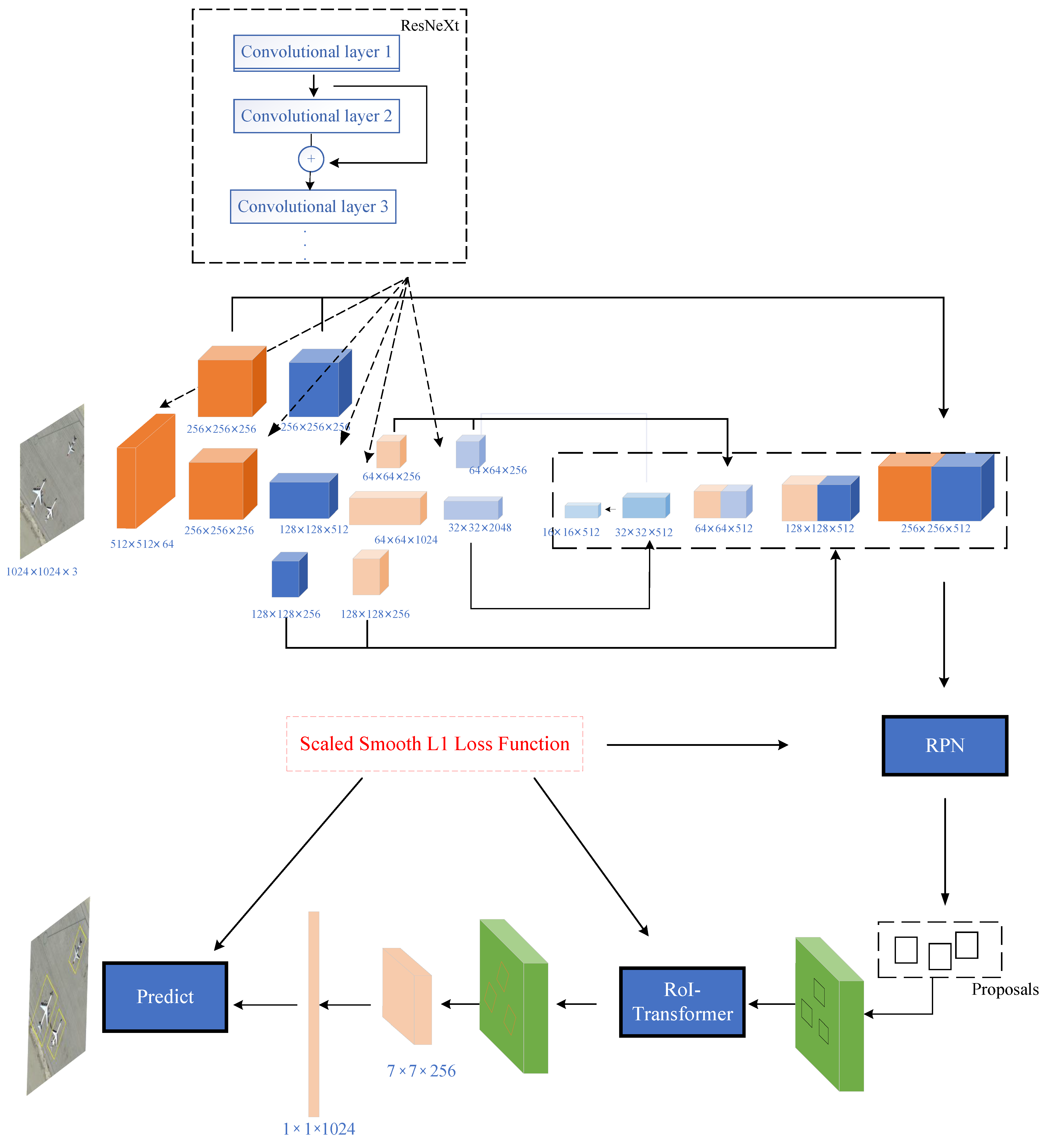
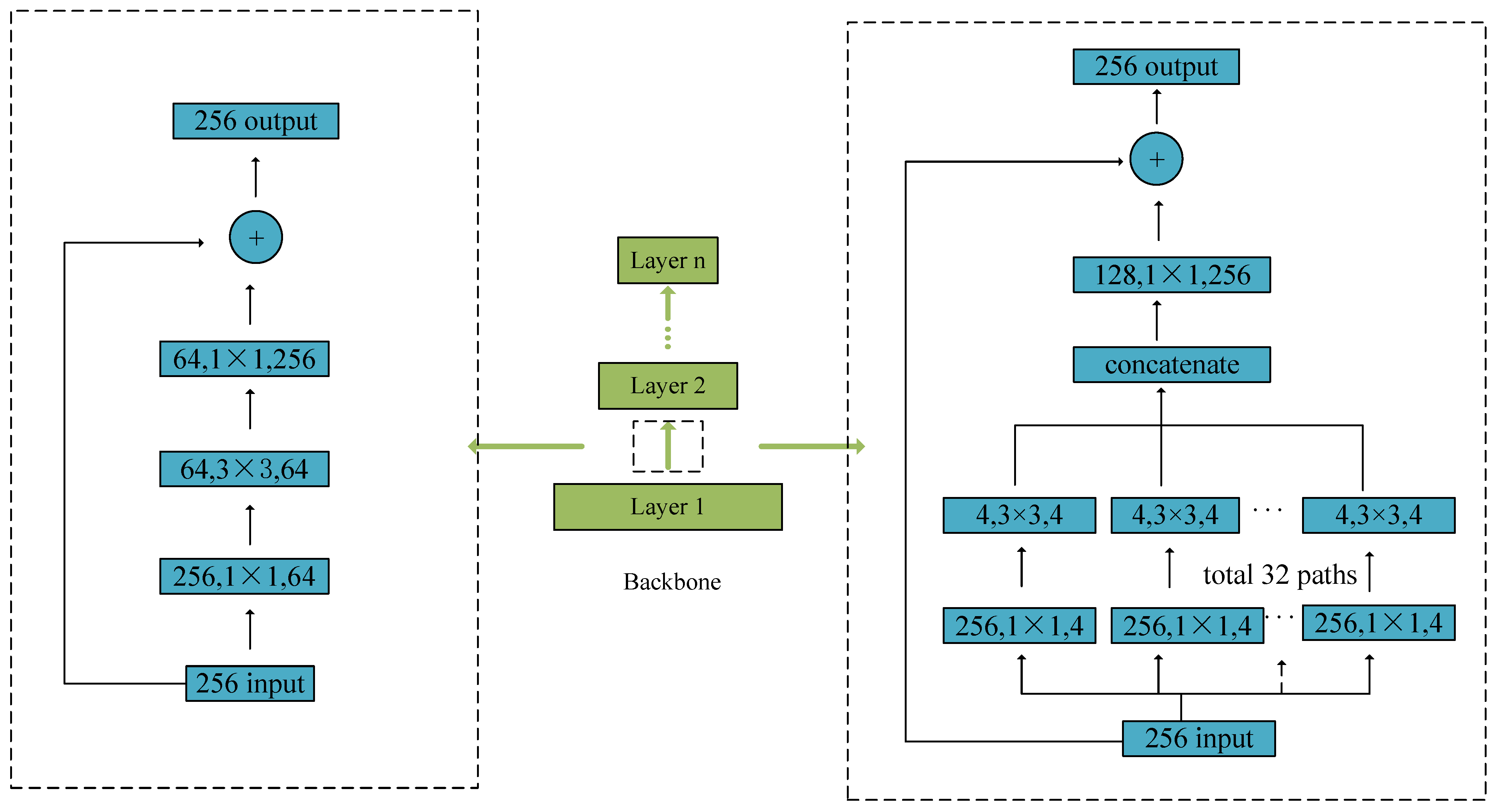
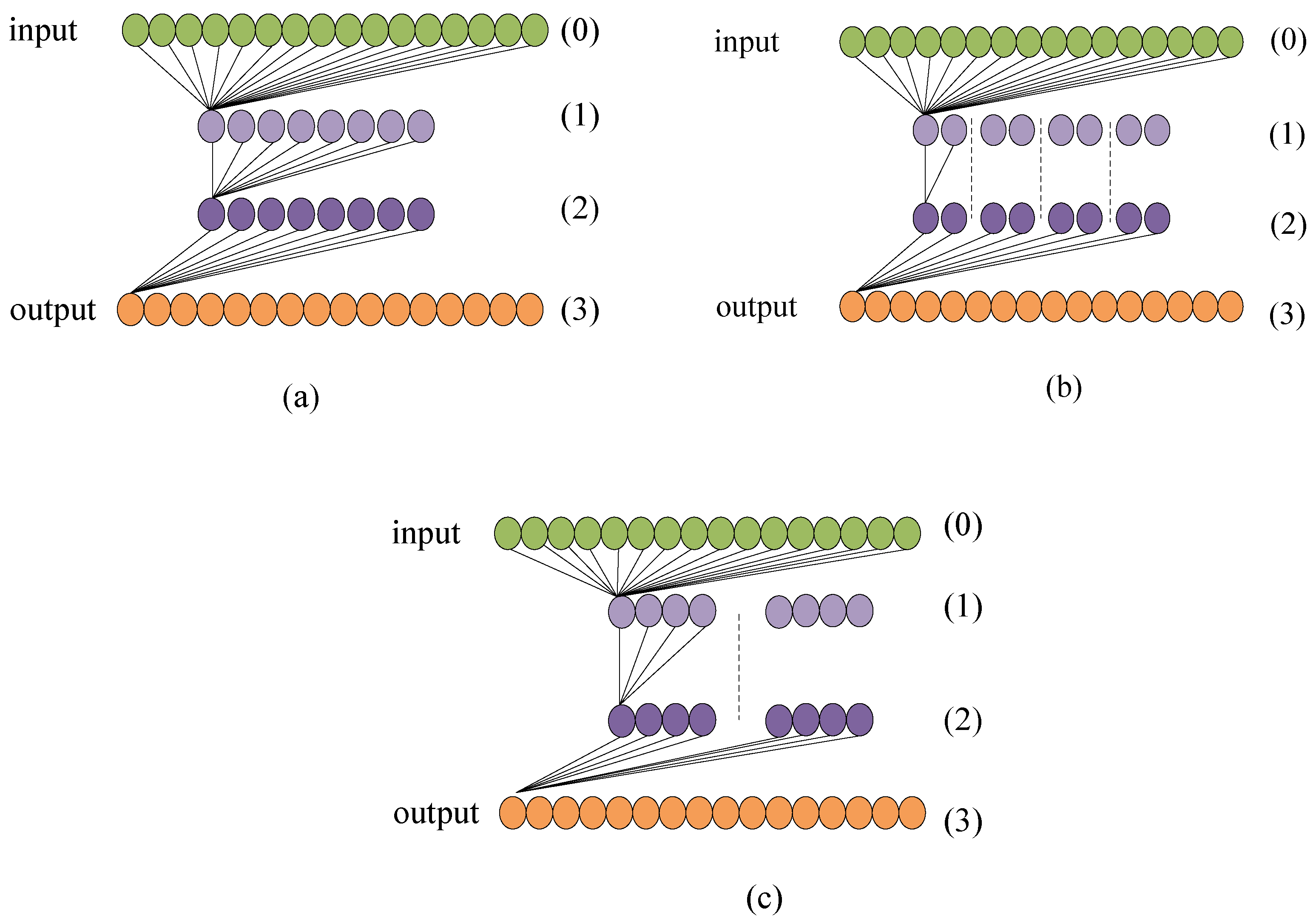
2.1. Feature Extraction Network

Since ResNet [53] adopts a shortcut connection structure, it has an advantage that the accuracy cannot degrade when the depth of the network increases. Hence, as a backbone, ResNet is popular in object detection architecture. Xie et al. [56] proposed a novel backbone named ResNeXt, which is more efficient than ResNet since it employs the split–transform–merge structure involved in the family of inception models [65,66]. For detailed units of ResNet and ResNeXt, see Figure 5.

ResNeXt shares the same basic topology as that of ResNet, and extracts features from bottom–up with multiple convolution modules. As one more hyperparameter, the cardinality, which is used to control the number of splitting convolution modules, can be considered as a new dimension in the channel. Figure 5 shows that the input features of 256 channels can be divided into 32 groups of low-dimension features with 4 channels (i.e., cardinality = 32, width = 4) using 1 × 1 convolution. The output features can then merge the low-dimension features into high-dimension features using 1 × 1 convolution.

Compared with ResNet [53], ResNeXt [56] performs better. In [56], there are many experiments showing the effectiveness of ResNeXt. Nevertheless, compared with ResNet, few theoretical analyses about the effectiveness of ResNeXt have been studied in the literature. From the perspective of the algorithm, we provide here a theoretical analysis that shows that the ResNeXt should be more effective than ResNet.

In general, if an object detection model has more parameters to optimize, then the complexity is higher. Obviously, it contains two factors of the spatial space and channel space. The schematic principle of complexity can be seen from Figure 6. For example, we assume that the number of channels of input features is 16, the output is 16, the middle is 8 for ResNet as in Figure 6a, for ResNeXt (4 × 2) as in Figure 6b, and ResNeXt (2 × 4), as in Figure 6c, respectively. For simplicity, we define the 0^th layer, 1^th layer, 2^th layer, and 3^th layer. Then for Figure 6a, Flops can be computed, i.e., 16 × 8 in ($0^{\mathit{th}}\to 1^{\mathit{th}}$), 8 × 8 in ($1^{\mathit{th}}\to 2^{\mathit{th}}$), 8 × 16 in ($2^{\mathit{th}}\to 3^{\mathit{th}}$), and sum to $(16\times 8+8\times 8+8\times 16)$ flops. For Figure 6b, denoting ResNeXt (4 groups with width 2), Flops in $0^{\mathit{th}}\to 1^{\mathit{th}}$ is $(8\times 16)$, in $1^{\mathit{th}}\to 2^{\mathit{th}}$ is $(2\times 2\times 4)$, and in ($2^{\mathit{th}}\to 3^{\mathit{th}}$) is 8$\times 16$. For Figure 6c, representing ResNeXt (2 groups with a width of 4), the total Flops is $(8\times 16+4\times 4\times 2+8\times 16)$. Let $C_{in}$ denote the number of input feature channels, $C_{mid}$ the number of middle features, $C_{out}$ the output features, $C_{car}$ the cardinality, and B the width, respectively. Then, the complexities of ResNet and ResNeXt on channel can be computed, respectively, as follows:

$$\begin{array}{cc}\hfill & FLOP{s}_{resnet}=C_{in}\times C_{mid}+C_{mid}\times C_{mid}+C_{mid}\times C_{out}\hfill \\ \hfill & FLOP{s}_{resnext}=C_{in}\times (C_{car}\times B)+(B\times B\times C_{car})+C_{out}\times C_{car}\times B\hfill \end{array}$$

(1)

From (1), the computational complexity of ResNet and ResNeXt can be computed explicitly. As reported in [53,56], the complexity of ResNet is slightly lower than that of ResNeXt in the conv2 and conv3 stages due to the smaller number of input features. However, in the conv4 and conv5 stages, the complexity of ResNet becomes significantly higher than that of ResNeXt when the number of input feature channels increases. Therefore, the computational complexity of ResNeXt is generally lower than that of ResNet, which is why we choose ResNeXt as the backbone of our proposed method.

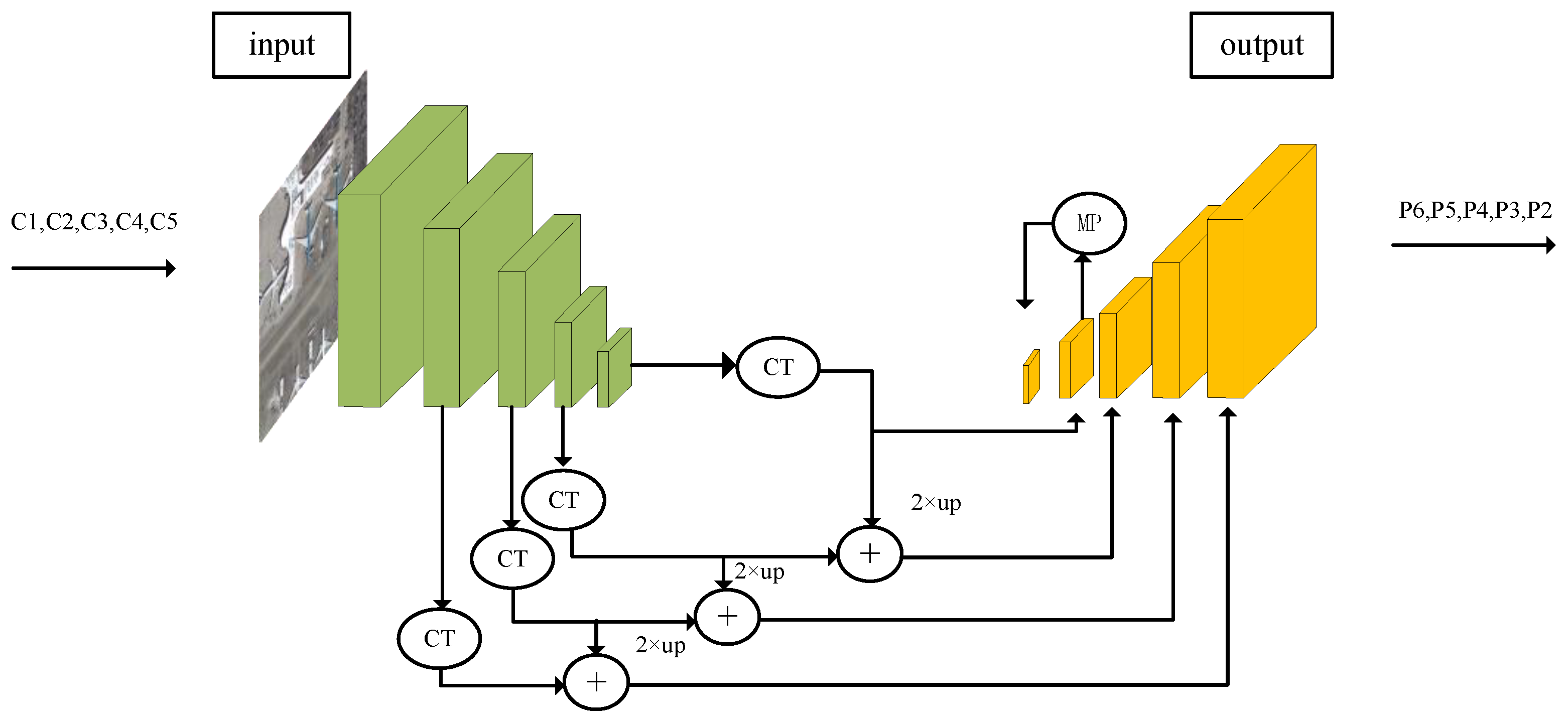
2.2. Feature Fusion Network

In object detection in remote sensing images, the performance of a detector is usually sensitive to the scale variant of the images. To deal with this issue, Lin et al. [20] proposed the feature pyramid net (FPN) to extract multi-scale features. Since then, the FPN has been widely applied to many networks to improve performance. Many experiments show the effectiveness of FPN, especially in small objects, which are important for object detection in remote sensing. Combining ResNeXt and FPN, the structure of extracting and fusing features is shown in Figure 7. By fusing multi-scale semantic formation, this architecture not only extracts rich features but also suppresses the vanish of the formation of small objects.

Figure 7 illustrates the bottom-up feature extraction and top-down feature fusion structure of FPN. FPN combines features of different spatial sizes through upsampling and fusion. The backbone generates feature maps C1, C2, C3, C4, and C5. The features from C2 to C5 are fused to create feature maps P2, P3, P4, and P5. P6 is obtained by applying a 3 × 3 convolution with a stride of 2 to P5. The features from high levels have larger receptive fields, making them more suitable for detecting larger objects. The features from lower levels, such as P3 and P4, are more efficient in detecting smaller objects with lower resolution. Under such a structure, we usually achieve good detection performance, especially in remote sensing image detection.

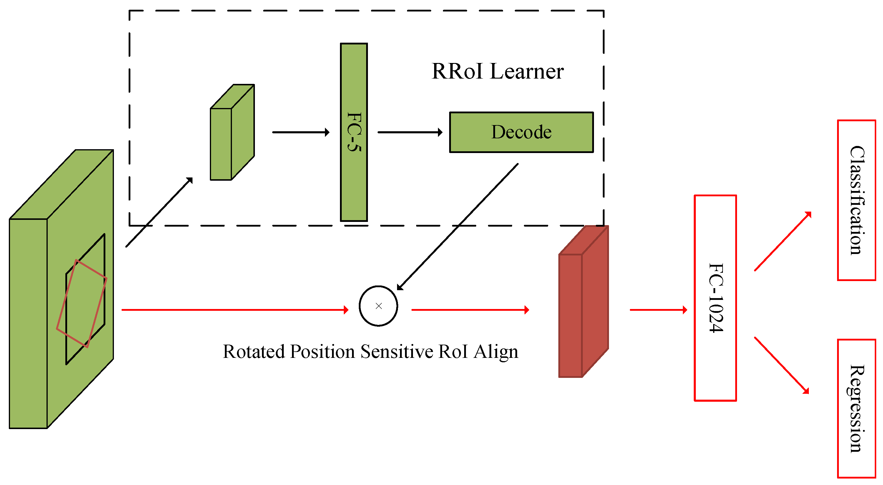
2.3. The Structure of the RoI-Transformer

Since the orientations of objects in remote sensing images are usually arbitrary, and most objects are often densely packed, as Figure 1 shows, the methods relying on horizontal proposals may struggle to achieve high location accuracy. At the head of the RoIs in the second stage, we employ the RoI-Transformer, proposed by Ding et al. [51], which is a powerful mechanism to obtain oriented bounding boxes.

The RoI-Transformer is a learnable module, which can transform HRoIs into RRoIs and avoid a large number of anchors designed for oriented object detection. Its structure is shown in Figure 8.

2.4. Rotated Bounding Box Regression and Classification

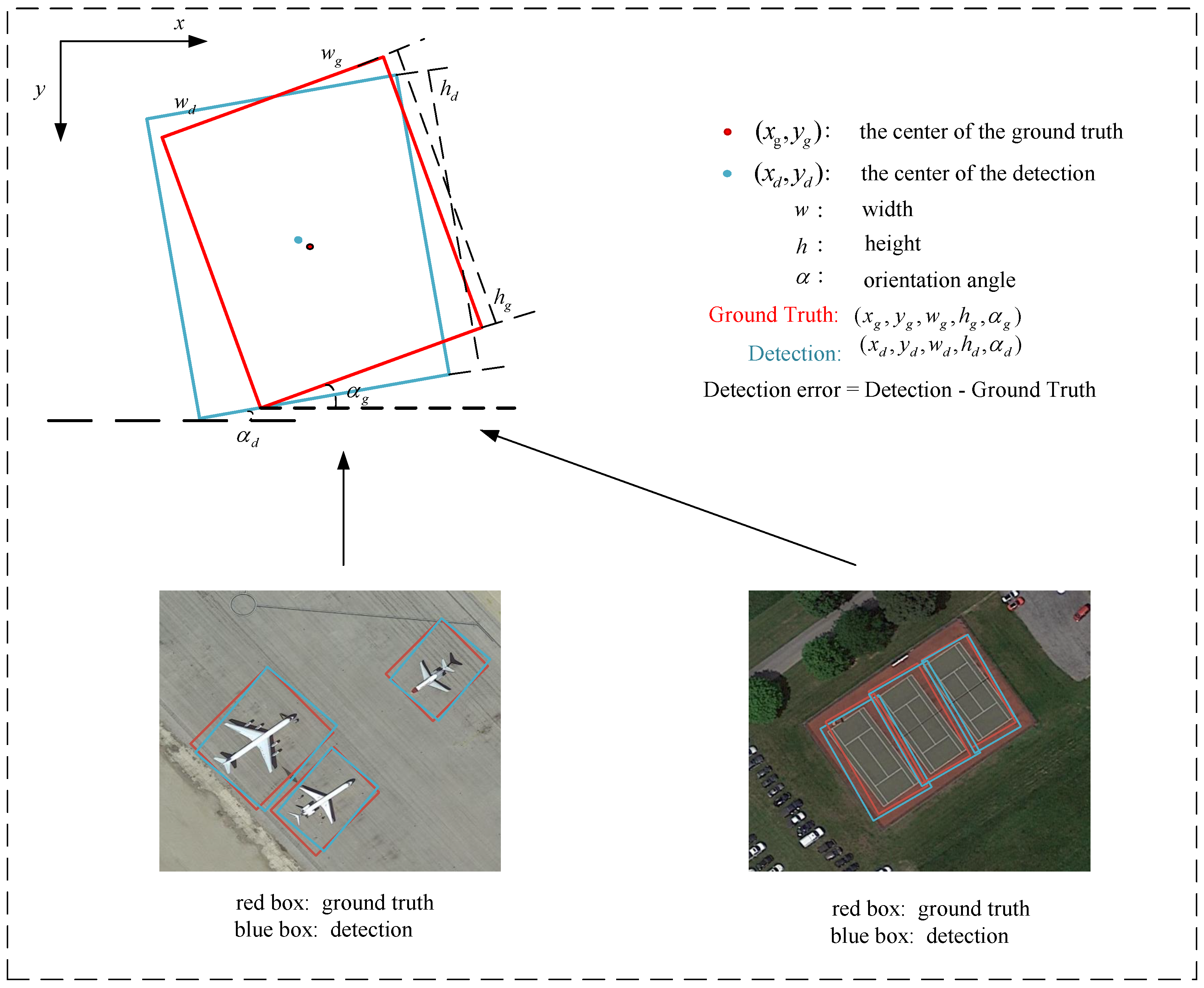
In this section, we will first introduce the scaled smooth L${}_1$ loss function in detail. Then, we describe the rotated bounding box regression and classification.

2.4.1. The Scaled Smooth L${}_1$ Loss Function

In this subsection, we will review the common smooth L${}_1$ loss function briefly, introduce the definition of the scale factor, and give the scaled smooth L${}_1$ loss function in detail.

The smooth L${}_1$ loss function is defined as

$$L_{loss}\left(x\right)=\left\{\begin{array}{cc}0.5x^2,\hfill & \left|x\right|<1,\hfill \\ \left|x\right|-0.5,\hfill & \left|x\right|\ge 1.\hfill \end{array}\right.$$

(2)

In the bounding box regression, the smooth L${}_1$ loss function operates on the detection error, i.e., the variable x of L${}_{loss}\left(x\right)$ represents the detection error. As mentioned previously, this smooth L${}_1$ loss function plays an important role in a two-stage detector because it is used to undertake the bounding box regression task. As pointed out in the introduction, the variance in the detection error ${\sigma }^2$ could affect the performance of a detector. On the other hand, we observe that the smooth L${}_1$ loss function L${}_{loss}\left(x\right)$ as in (2) has nothing to do with the variance ${\sigma }^2$. Taking into account the important role that a regression loss function takes in a two-stage approach, we manage to update the smooth L${}_1$ loss function to a new one, which should have something to do with the variance ${\sigma }^2$. We suggest the use of the scaled smooth L${}_1$ loss function L${}_{sloss}\left(x\right)$, which is defined as

$$L_{sloss}\left(x\right)=\left\{\begin{array}{cc}0.5{\left(\frac{x}{\sigma }\right)}^2,\hfill & \left|x\right|<1,\hfill \\ |\frac{x}{\sigma }|-0.5,\hfill & \left|x\right|\ge 1,\hfill \end{array}\right.$$

(3)

where $\sigma >0$ is now a pre-specified constant, and is referred to as the scale factor. Notice that when $\sigma$ is set to 1, then the scaled smooth L${}_1$ loss function becomes the common smooth L${}_1$ loss function. Under this scaled smooth L${}_1$ loss function, the corresponding variance in the detection error becomes 1; it appears that we scale any variance in the detection error to 1. This is also why we call the constant $\sigma$ the scale factor.

Now, we can provide an alternative explanation for the role that the scale factor $\sigma$ takes in L${}_{sloss}$. Notice that when the scaled smooth L${}_1$ loss function is used to undertake the bounding box regression, the variable x of L${}_{sloss}\left(x\right)$ will represent the detection error. If we regard $\frac{1}{{\sigma }^2}$ and $\frac{1}{\sigma }$ as two weights, then L${}_{sloss}$ can be considered as such a loss function that endows weight $\frac{1}{{\sigma }^2}$ and $\frac{1}{\sigma }$ to the L${}_2$ loss term (i.e., term $x^2$) and L${}_1$ loss term (i.e., term $\left|x\right|$), respectively. By (3), we can obtain the gradient formula for L${}_{sloss}$ as follows:

$$\frac{\partial L_{sloss}\left(x\right)}{\partial x}=\left\{\begin{array}{cc}\pm \frac{1}{{\sigma }^2}\left|x\right|,\hfill & \left|x\right|<1,\hfill \\ \pm \frac{1}{\sigma },\hfill & \left|x\right|\ge 1.\hfill \end{array}\right.$$

(4)

Compared with that of L${}_{loss}$, L${}_{sloss}$ raises the ratio of gradients, $\sigma /\left|x\right|$, between parts of $\left|x\right|\ge 1$ and $\left|x\right|<1$, when $\sigma >1$. In other words, the scaled smooth L${}_1$ loss function $L_{sloss}$ focuses more on suppressing the large detection error and, thus, improve the object location accuracy.

By controlling the value of the scale factor $\sigma$, we should be able to improve the performance (say, overall mAP) of the detectors. Experimental results will support our viewpoint, and indicate that the optimal scale factor is about 2.0, rather than the commonly used 1.0 corresponding to the common smooth L${}_1$ loss function.

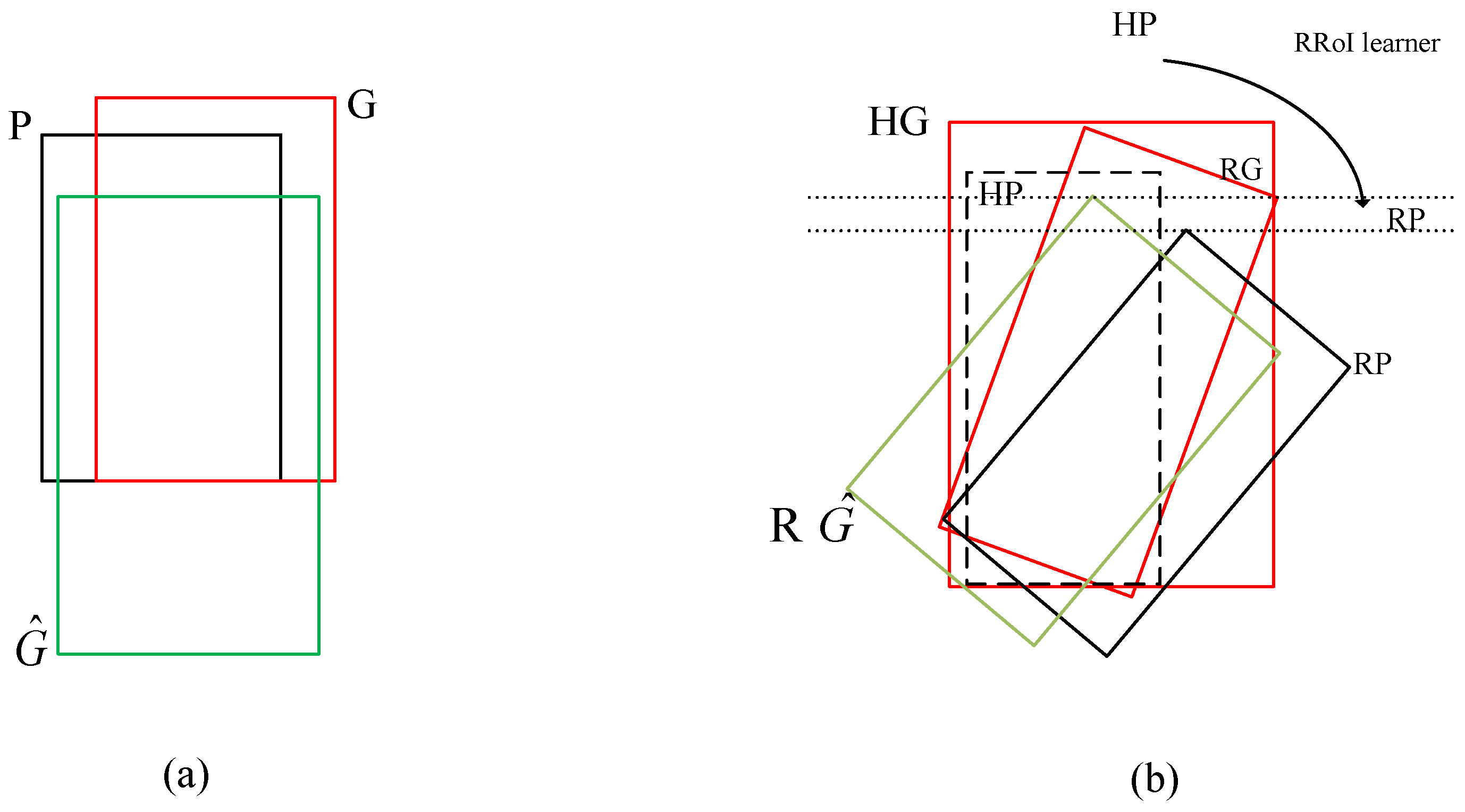
2.4.2. Rotated Bounding Box Regression

As pointed out previously, in a two-stage object detection architecture, the horizontal bounding boxes are most likely not suitable for detecting oriented and densely packed objects, especially in aerial image object detection. Hence, in this study, instead of using horizontal bounding boxes to generate candidate object locations, we used rotated bounding boxes, see Figure 9. Next, we describe in detail the rotated bounding box regression, which has some similarities to work by Ding et al. [51]. First, we acquire horizontal bounding boxes (i.e., horizontal proposals) from the RPN. Denote by HG and HP the horizontal ground-truth bounding box and horizontal proposal, respectively. By the RoI-Transformer, we learn from HP to obtain the rotated proposal ($RP$, i.e., rotated bounding box). Denote by $RG$ the rotated ground-truth bounding box. The input to our training algorithm is a set of N training samples ${\{R{P}^i,R{G}^i\}}_{i=1,\cdots ,N}$, where $R{P}^i={(x_{R{P}^i},y_{R{P}^i},w_{R{P}^i},h_{R{P}^i},{\theta }_{R{P}^i})}^{\mathrm{T}}$, where the superscript $\mathrm{T}$ means the transpose of a vector, among which $(x_{R{P}^i},y_{R{P}^i})$ specifies the coordinates of the center of rotated proposal $R{P}^i$, $w_{R{P}^i}$ and $h_{R{P}^i}$ represent the width and height of $R{P}^i$, respectively, and ${\theta }_{R{P}^i}$ specifies the orientation of $R{P}^i$. From now on, we drop the superscript i unless it is necessarily stated. The task of the rotated bounding box regression is to learn a transformation that assigns a rotated proposal $RP$ to a rotated ground–truth bounding box $RG$.

To facilitate the learning transformation, the transformation is parameterized by means of five functions ${\widehat{t}}_x\left(RP\right)$, ${\widehat{t}}_y\left(RP\right)$, ${\widehat{t}}_w\left(RP\right)$, ${\widehat{t}}_h\left(RP\right)$, and ${\widehat{t}}_{\theta }\left(RP\right)$. The first two functions represent the transformation of the center of $RP$. ${\widehat{t}}_w\left(RP\right)$ and ${\widehat{t}}_h\left(RP\right)$ represent log-space transformations of the width and height of $RP$, respectively, while $\widehat{t_{\theta }}\left(RP\right)$ stands for the normalized $2\pi$-space transformation of the orientation of $RP$. Once we learn these functions, with an input $RP$, we can predict a candidate $R\widehat{G}=(x_{R\widehat{G}},y_{R\widehat{G}},w_{R\widehat{G}},h_{R\widehat{G}},{\theta }_{R\widehat{G}})$ for a rotated ground-truth $RG$, which can be obtained by the following formulas:

$$\begin{array}{cc}\hfill & x_{R\widehat{G}}=cos{\theta }_{RP}·{\widehat{t}}_x\left(RP\right)·w_{RP}-sin{\theta }_{RP}·{\widehat{t}}_y\left(RP\right)·h_{RP}+x_{RP},\hfill \\ \hfill & y_{R\widehat{G}}=sin{\theta }_{RP}·{\widehat{t}}_x\left(RP\right)·w_{RP}+cos{\theta }_{RP}·{\widehat{t}}_y\left(RP\right)·h_{RP}+y_{RP},\hfill \\ \hfill & w_{R\widehat{G}}=exp\left({\widehat{t}}_w\left(RP\right)\right)·w_{RP},h_{R\widehat{G}}=exp\left({\widehat{t}}_h\left(RP\right)\right)·h_{RP},\hfill \\ \hfill & {\theta }_{R\widehat{G}}=(2\pi {\widehat{t}}_{\theta }(\left(RP\right)+{\theta }_{RP},mod2\pi ).\hfill \end{array}$$

(5)

Next, we address how to learn those five functions ${\widehat{t}}_{*}\left(RP\right)$ from $RP$, where * can be one of $x,y,w,h,\theta$. To ensure that the rotated bounding box regression is effective and efficient, ${\widehat{t}}_{*}\left(RP\right)$ we use a linear function of features of $RP$, i.e., ${\hat{t}}_{*}\left(RP\right)={\hat{\mathit{w}}}_{*}^{\mathrm{T}}\left(RP\right)$, where ${\hat{\mathit{w}}}_{*}$ is a column vector of learnable model parameters. We learn ${\hat{\mathit{w}}}_{*}$ by optimizing the following optimal model:

$${\hat{\mathit{w}}}_{*}=\underset{{\mathit{w}}_{*}}{argmin}\sum _{i=1}^N{L}_{reg}(t_{*}^i,{\mathit{w}}_{*}^{\mathrm{T}}\left(R{P}^i\right)),$$

(6)

where $L_{reg}$ is a loss function, and $t_{*}$ is defined as:

$$\begin{array}{cc}\hfill & t_x=((x_{RG}-x_{RP})·cos{\theta }_{RP}+(y_{RG}-y_{RP})·sin{\theta }_{RP})/w_{RP},\hfill \\ \hfill & t_y=((y_{RG}-y_{RP})·cos{\theta }_{RP}-(x_{RG}-x_{RP})·sin{\theta }_{RP})/h_{RP},\hfill \\ \hfill & t_w=log\left(\frac{w_{RG}}{w_{RP}}\right),t_h=log\left(\frac{h_{RG}}{h_{RP}}\right),\hfill \\ \hfill & t_{\theta }=\frac{1}{2\pi }·(({\theta }_{RG}-{\theta }_{RP}),mod2\pi ).\hfill \end{array}$$

(7)

As pointed out previously, in order to ensure the regression (i.e., the optimal model (6)) efficient, the loss function $L_{reg}$ operates on the vector $\Delta =t_{*}-{\mathit{w}}_{*}^{\mathrm{T}}\left(RP\right)$, i.e., $L_{reg}(t_{*},{\mathit{w}}_{*}^{\mathrm{T}}\left(RP\right))=L_{sloss}(\Delta )$, where $L_{sloss}(·)$ is the scaled smooth $L_1$ loss function as in Formula (3).

2.4.3. Classification

The total loss of the model consists of two parts. One is the location loss computed above, the other is the classification one. The classifier is a function $\theta \left(RP\right)$ of $RP$, which assigns each $RP$ (rotated proposal) a label among the $M+1$ classes. Class 0 is background, the other M classes correspond to objects to detect. $\theta \left(RP\right)$ is an $(M+1)$-dimensional estimate of the posterior distribution over classes, i.e., for a $RP$, ${\theta }_k\left(RP\right):=P(y=k|RP)$, where y is the class label, $k=0,1,...,M$. Given N training samples ${(y^i,R{P}^i)}_{i=1,...,N}$, we minimize the classification loss to learn the classifier $\theta$, i.e.,

$$\widehat{\theta }=\underset{\theta }{argmin}\sum _i^N{L}_{cls}(y^i,\theta \left(R{P}^i\right)),$$

(8)

where the classification loss function $L_{cls}$ is the cross-entropy, as follows:

$$L_{cls}(y,p)=-logp,$$

(9)

where p is the estimated probability for the class with label y.

3. Experimental Settings and Implementation Details

In this section, we briefly introduce the experimental settings, including experimental settings, experiment platforms, datasets, evaluation metrics, and implementations.

• Experimental Platform: In order to evaluate the performance of the proposed method comprehensively and provide baseline, a normal experimental platform is used. The environments are Intel i7-9750, memory 20 GB, a single NVIDIA Tesla V100 GPU with 16 GB of memory, along with the PyTorch 1.1.0 and Python 3.7.
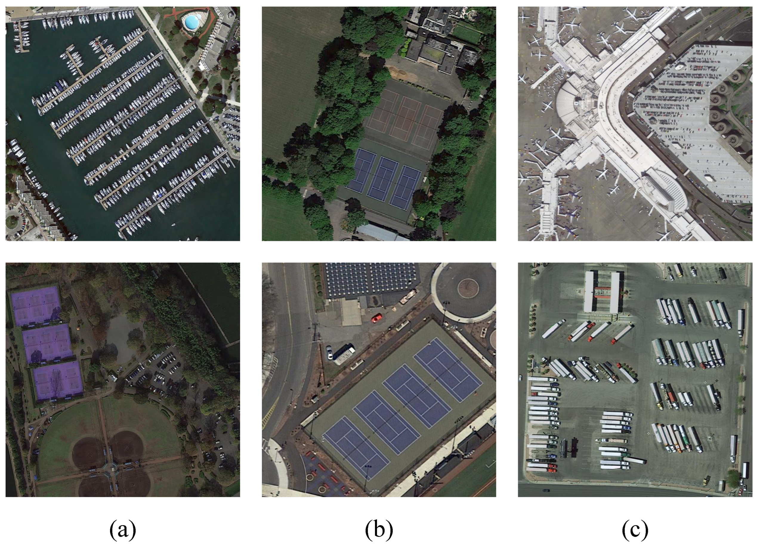
• Datasets: The DOTA [38] dataset is a public open-access dataset for object detection in aerial images at large scales. It provides two kinds of annotations for oriented and horizontal bounding boxes, respectively. The aerial images of DOTA are collected from Google Earth and satellites, including Julang-1(JL-1) and GF-2. DOTA contains 2806 aerial images. It consists of a training set (1411 images), validation set (458 images), and testing set (937 images). The sizes of the images change from 800 × 800 pixels to 4000 × 4000 pixels. There are 188,282 instances including plane (PL), basketball diamond (BD), bridge (BR), ground field track (GFT), small vehicle (SV), large vehicle (LV), ship (SH), tennis court (TC), basketball court (BC), storage tank (ST), soccer ball field (SBF), roundabout (RA), harbor (HA), swimming pool (SP), and helicopter (HC), 15 categories in total.

DOTA is now one of the largest and most widely used high-resolution aerial remote sensing datasets. The instances in DOTA change greatly in scale, orientation, and aspect ratio; small objects are usually oriented and densely packed. Hence, the DOTA has the characteristics of diverse categories, scales, and sensor sources. Therefore, it is a very difficult and challenging task to detect objects in this dataset.

We used the training set and validation set with annotations for training and the online testing set for testing (since the annotations of testing set were undisclosed).

The HRSC2016 dataset is a publicly available dataset for object detection in aerial images, proposed by [67]. It contains 1070 images collected from Google Earth, featuring over 20 types of ships with various scales, positions, rotations, and appearances. The dataset also provides labels of rotated bounding boxes. The image sizes in the dataset range from 300 × 300 to 1500 × 900. The training, validation, and testing sets contain 443 images with 1207 samples, 183 images with 544 samples, and 444 images with 1071 samples, respectively.

Compared with DOTA dataset, the HRSC2016 dataset consists of a single object category—the ship. Nevertheless, since the instances of HRSC2016 in the rotation, scale, location, shape, and appearance have change a lot, it is also difficult and challenging to detect the objects in this dataset.

During the training, we only adopted horizontal flipping (as with a DOTA dataset) for data augmentation. The images were cropped into sub-images of 800 × 800 pixels.

• Evaluation Metrics: In object detection, precision and recall are commonly used to evaluate the effectiveness of a method in addition to mean average precision (mAP). We also adopted precision and recall to comprehensively evaluate the effectiveness of the proposed method. Precision is an indicator that represents the percentage of detected objects that are ’ground-truth’. The recall reflects the ratio with which all true samples can be rightly detected. More precisely, the precision and recall are calculated as follows:

  $$precision=\frac{TP}{TP+FP},$$

  (10)

  $$recall=\frac{TP}{TP+FN},$$

  (11)

  where TP is the number of targets the model predicts correctly, FP denotes the number of targets predicted incorrectly, FN is the number of targets predicted incorrectly with the true label. With precision and recall, the AP can be defined by

  $$AP\left(u\right)={\int }_0^{1}p\left(r_u\right)d{r}_u,$$

  (12)

  where u represents class u, $r_u$ is the recall for class u, $p\left(r_u\right)$ denotes the precision corresponding to the recall $r_u\in [0,1]$. mAP is the average of classes ${}^{\prime }$ AP, which is an indicator reflecting the comprehensive performance. The calculation for mAP is as follows:

  $$mAP=\frac{1}{N}\sum _{u=1}^{N}AP\left(u\right),$$

  (13)

  where N represents the number of the total categories.
• Implementation: To better evaluate the performance of our method, the hyperparameters in our experiments are set to be the same. The batch size is set at 2. The initial learning rate is $0.01$. The momentum is $0.9$. The weight decay is $0.0001$ and the optimization strategy is the SGD (stochastic gradient decent) algorithm [68]. The normalization strategy is batch normalization [69]. The initial weight of the backbone is pre-trained on the ImageNet [70] dataset.

4. Experimental Results and Analysis

On two datasets DOTA [38] and HRSC2016 [37], experiments are implemented to demonstrate the effectiveness of the proposed method. First, we introduce the experiment conditions. Second, on the DOTA dataset [38], we evaluate the influence of the backbone on the performance of the proposed architecture. Third, we analyze the optimal scale factor by experimenting on DOTA [38], and the optimal scale factor is also justified on HRSC2016 [37]. Finally, comparisons of the proposed algorithm with other frameworks are discussed.

4.1. Effective Experiments

We used ResNeXt as the backbone and FPN as the neck in the Faster R-CNN framework, replacing the ResNet backbone used in previous methods. The ResNeXt backbone was pre-trained on ImageNet, and the FPN allowed for information extraction from multi-spatial features. In the RPN stage, we designed anchors with 3 different aspect ratios (0.5, 1.0, 2.0) and a single scale ratio of 12. To reduce memory requirements, we cropped the high-resolution DOTA dataset images into a series of 1024 × 1024 patches.

Figure 10 shows the variation of losses in the training process, which includes three stages: the RPN stage, the RoI-Transformer stage, and the final stage.

Figure 10d shows the blue curve, representing the overall total loss, which aggregates all losses including both loc and cls losses of all three RPN, RoI-Transformer, and final predict stages during training. As the iterations increase, the overall total loss rapidly decreases and becomes almost flat with little fluctuation. This indicates that the minimizing the overall total loss procedure is successfully completed, and the corresponding optimal model parameters are acquired by training, making our method trainable and stable. A similar description applies to Figure 10a–c, where the loc and cls losses correspond to RPN, RoI-Transformer, and final predict stages, respectively, instead of the overall sense as in Figure 10d.

Some object detection results of our method on the DOTA dataset [38] are demonstrated in Figure 11.

As shown in Figure 11, our method can correctly detect a majority of the instances. The recognized objects are marked by colorful and oriented rectangular boxes, and their categories are predicted. In the test dataset, various objects are featured from various aspects. The objects vary in size and visibility depending the distance between the objects and the sensors. Therefore, more detailed RBBs rather than HBBs are needed to correctly detect those targets which are small, oriented and densely packed. The proposed algorithm can decrease the detection error caused by external environmental factors. In summary, our method is effective in object detection, i.e., in multi-scale remote sensing imaging and crowd-arbitrary environments.

4.2. Comparisons and Analysis of Different Backbones

The performances with various backbones ResNet50, ResNet101, ResNeXt50, and ResNeXt101 were evaluated by using our detector—Faster R-CNN with RoI-Transformer—to experiment on the DOTA dataset.

Table 1. Comparison of different backbones.

Backbone	PL	BD	BR	GTF	SV	LV	SH	TC	BC	ST	SBF	RA	HA	SP	HC	mAP
ResNet50	80.66	73.15	42.70	65.44	71.73	71.23	76.18	90.31	83.25	73.41	51.02	56.97	63.78	61.93	49.37	67.41
ResNet101	80.60	77.74	44.82	67.51	72.24	71.93	75.29	90.54	84.36	74.55	50.61	61.33	65.16	66.20	55.46	69.22
ResNet101 *	80.47	75.18	42.07	67.30	72.08	71.74	67.86	90.01	78.84	68.98	48.56	61.35	63.76	68.18	55.32	67.45
ResNeXt50	87.13	74.61	45.56	70.73	72.60	72.22	75.37	90.05	84.31	75.80	49.94	61.85	66.33	65.67	54.85	69.80
ResNeXt101	80.72	76.95	44.58	70.35	72.55	73.23	75.66	90.54	80.83	75.67	49.53	59.38	65.86	66.59	51.64	68.94
ResNeXt101 *	80.27	76.19	44.37	67.18	72.56	72.68	67.99	90.39	81.21	75.59	45.27	59.75	64.81	66.91	51.79	67.81

* stands for being trained by 24 epochs.

shows the results of different backbones including the $AP$ values of 15 categories and an mAP measurement online officially. During the experiment, we used the training and validation datasets for training, and the test dataset for testing. The loss function for regression is set to the common smooth $L_1$ loss function, i.e., $\sigma =1.0$ as in Formula (2).

Compared with ResNet50 and ResNeXt50, ResNet101 and ResNeXt101 go deeper. Thus, ResNet101 and ResNeXt101 are separately trained by 12 and 24 epochs, respectively. Note that the performances of training 24 epochs are marked by the star sign. The others are trained by 12 epochs. From Table 1, we can find that the performance of our method with backbone ResNeXt50 is the best with a mAP of 69.8, which is consecutively higher than others by gaps of mAPs of 2.39, 0.58, 2.35, 0.86, and 1.99, respectively. The experimental results also suggest that a backbone with more layers does not necessarily result in a better performance. This phenomenon is most likely due to over-fitting in training, which results in an insufficient generalization ability in testing. At the same time, the network with ResNeXt50 also achieves the highest $APs$ of about half of the 15 categories, for example, PL, BR, and so on. In the following experiments, the backbone in our detector is set as ResNeXt50.

4.3. Analysis of Performance under Different Scale Factors

As pointed out in Section 2.4.2, we suggest using the scaled smooth $L_1$ loss function in regression instead of the common smooth $L_1$ loss function. We now focus on the investigation of the impact of the scale factor $\sigma$ on the performance of our algorithm, and, consequently, look for the optimal scale factor on the DOTA [38] dataset.

Table 2. Performances under different scale factors $\sigma$.

$\mathit{\sigma }$	PL	BD	BR	GTF	SV	LV	SH	TC	BC	ST	SBF	RA	HA	SP	HC	mAP
0.5	81.34	74.69	43.78	63.78	71.95	72.08	75.29	89.70	85.30	74.21	49.39	59.21	65.53	58.58	52.07	67.79
1.0	87.13	74.61	45.56	70.73	72.60	72.22	75.37	90.05	84.31	75.80	49.94	61.85	66.33	65.67	54.85	69.80
1.5	86.47	78.73	45.19	70.01	72.12	72.46	68.62	90.37	84.77	76.03	54.76	60.28	66.09	68.66	58.57	70.21
2.0	87.32	80.15	45.93	68.98	72.46	72.68	76.02	90.60	84.61	75.82	53.34	62.24	65.84	68.82	57.52	70.82
2.5	86.81	76.10	46.35	70.18	72.76	72.60	75.61	90.71	84.58	74.38	49.03	61.22	65.94	68.65	58.46	70.23
3.0	87.26	76.32	45.53	69.90	71.95	73.21	69.01	90.74	82.77	76.21	49.29	62.20	66.11	68.84	57.35	69.78

shows the performances under different values of the scale factor $\sigma$, where we take our detector Faster R-CNN-ReXt with RoI-Transformer as the baseline and ResNeXt50 as the backbone, and set IoU = 0.5 in testing. Meanwhile, we use the training and validation datasets for training, and the testing dataset for testing.

From Table 2, we can see that under the case of IoU = 0.5, the optimal value of the scale factor $\sigma$ is 2 in the sense of best effectiveness. When $\sigma$ is set to be 2, we achieve a mAP of 70.82, which outperforms the other cases of $\sigma =0.5,1.0,1.5,2.5$, and 3, respectively, by gaps of 3.03, 1.02, 0.61, 0.59, and 1.04, respectively.

Figure 12 shows the visualization of object detection with different scale factors $\sigma$. The left, middle, and right columns correspond to $\sigma$ values of 1.0, 2.0, and 3.0, respectively. The detection results in the middle and right columns are more effective than those in the left column. For instance, in Figure 12a ($\sigma =1.0$), the rotated bounding boxes do not fit the objects very well. In contrast, in Figure 12a ($\sigma =2.0$) and ($\sigma =3.0$), the rotated bounding boxes fit the objects better. Similar observations are applicable to the detection results displayed in Figure 12c. For the detection results shown in the middle row (i.e., Figure 12b), we can see that more small objects are successfully detected with $\sigma =2.0$ and $3.0$, while some small objects cannot be detected with $\sigma =1.0$.

In summary, from the visualization of detection results, we can also demonstrate that the optimal scale factor for the best effectiveness should be $2.0$, which is in accordance with the quantitative evaluation of the performance shown in Table 2. These visualizations also indicate that the effect of the scale factor $\sigma$ is large for aerial image object detection, and that a larger scale factor than $1.0$ can result in better detection performance. The reason leading to the above phenomenon is mainly due to the fact that small, oriented, and densely packed objects usually appear in aerial images, which could cause a large variance in the regression error during the bounding box regression stage.

4.4. Comparisons and Analysis of Different Frameworks

In order to show the effectiveness of our model, we also compare the performances of our algorithm with other popular networks. The networks we chose were Faster R-CNN trained with OBBs [38], RRPN [40], R${}^2$CNN [71], and the RoI-Transformer [51]. The results on the DOTA dataset are shown in

Table 3. Comparisons of different detection methods.

Method	PL	BD	BR	GIF	SV	LV	SH	TC	BC	ST	SBF	RA	HA	SP	HC	mAP
FR-O [38]	79.42	77.13	17.7	64.05	35.3	38.02	37.16	89.41	69.64	59.28	50.30	52.91	47.89	47.40	46.30	54.33
RRPN [40]	80.94	65.75	35.34	67.44	59.92	50.91	55.81	90.67	66.92	72.39	55.06	52.23	55.14	53.35	48.22	61.01
R${}^2$CNN [71]	88.52	71.20	31.66	59.30	51.85	56.19	57.25	90.81	72.84	67.38	56.69	52.84	53.08	51.94	53.58	60.67
RoI-Trans * [51]	88.64	78.52	43.44	75.92	68.81	73.68	83.59	90.74	77.27	81.46	58.39	53.54	62.83	58.93	47.67	69.56
Ours	87.32	80.15	45.93	68.98	72.46	72.68	76.02	90.60	84.61	75.82	53.34	62.24	65.84	68.82	57.52	70.82

* means multi-scale testing.

.

Table 3 compares the performance of our proposed method with other state-of-the-art methods on DOTA dataset. FR-O [38] is a classic two-stage framework, while RRPN [40] and R2CNN [71] were originally designed for text scene detection. The results in Table 3 are the versions re-implemented by a third-party [51]. RoI-Transformer is a method specifically designed for remote sensing object detection. Our proposed method achieves an mAP of 70.82, which outperforms FR-O, RRPN, R${}^2$CNN, and RoI-Transformer by an average of 16.49, 9.81, 10.15, and 1.26, respectively. Note that RoI-Trains * uses multi-scale testing, whereas our model does not adopt a multi-scale strategy because the emphasis of this paper is to study the effect of the scale factor $\sigma$ on the performance, and to look for the optimal scale factor $\sigma$. Our proposed method achieves a higher mAP than RoI-Trans, demonstrating its comprehensive effectiveness.

4.5. The Validation Experiments on Other Datasets

In order to further verify the effectiveness of our method, we also implement experiments on the HRSC2016 dataset. The results are shown in

Table 4. Results of the HRSC2016 dataset.

Scale Factor $\mathit{\sigma }$	mAP	Precision	Recall
1.0	85.3	55.75	90.48
2.0	87.1	65.17	91.66
3.0	86.5	65.03	90.48

including recall, precision, and mAP of the ship.

From Table 4, we can see that the effect of the scale factor $\sigma$ on the performance of our method experimented on the HRSC2016 dataset is in line with that experimented on the DOTA dataset. Precisely, the precision increases in general when the scale factor $\sigma$ becomes larger, while the recall varies slowly. As a result, when the scale factor $\sigma$ is equal to $2.0$, we achieve the highest mAP of 87.1.

Table 5. Comparisons with other classical methods on HRSC2016.

Method	RC2 [47]	R${}^2$PN [41]	RRD [72]	RoI-Trans [51]	Ours
mAP	75.7	79.6	84.3	86.2	87.1

shows the comparisons of our method with some classical methods on the HRSC2016 dataset.

As shown in Table 5, our method with scale factor $\sigma$ 2.0 has the highest mAP of 87.1, which has improvements of 11.4, 7.5, 2.8, and 0.9 compared with RC2, R${}^2$PN, RRD, and RoI-Transformer, respectively. Some visualizations of the results of our algorithm on the HRSC2016 test dataset are displayed in Figure 13.

4.6. Discussion

While our experiments and analysis demonstrate the effectiveness of our model, there are still limitations that are worth discussing, as follows:

(I)

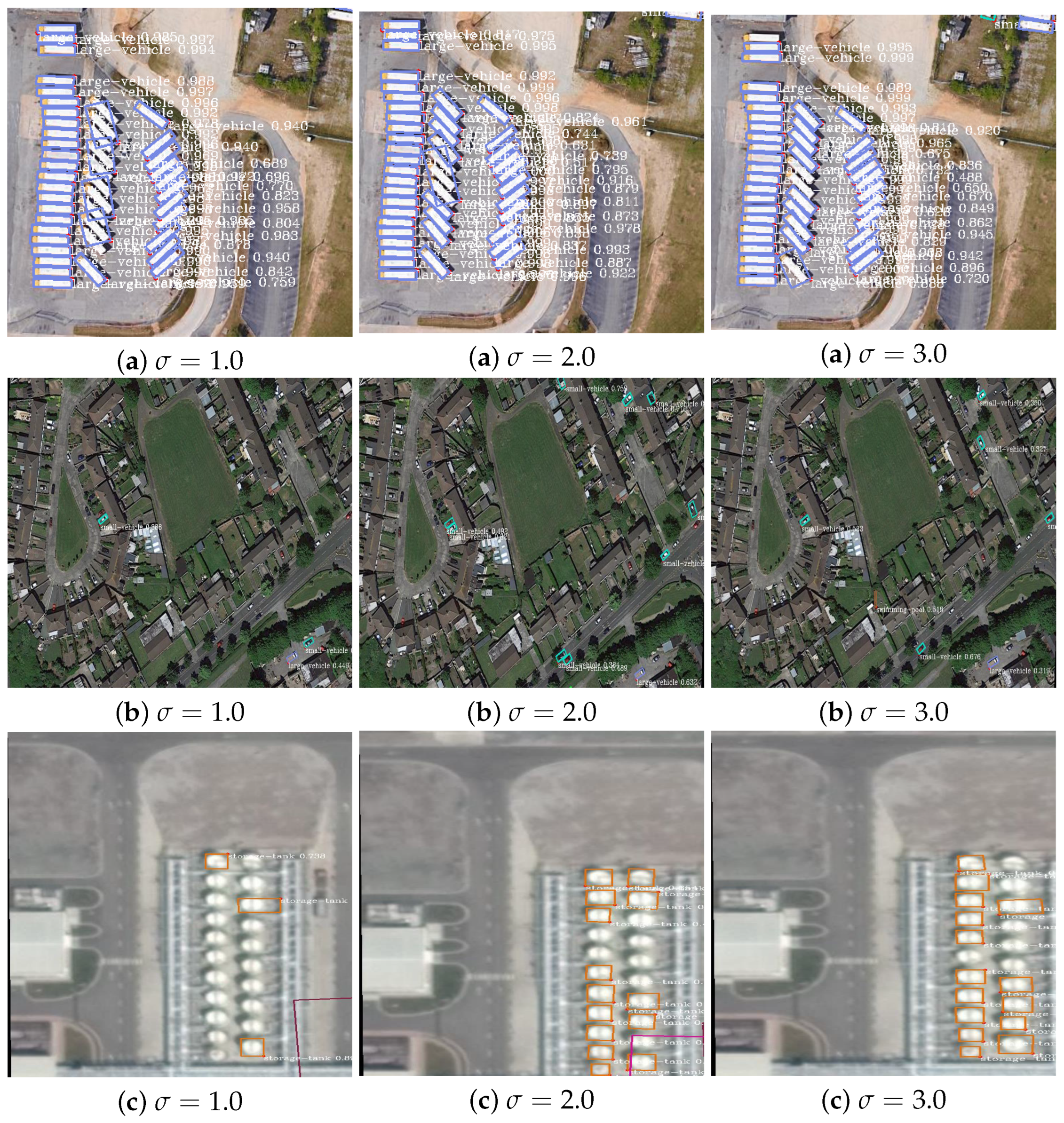
As described in Section 2.4.1, the scale factor $\sigma$ is pre-specified, and it corresponds to the whole collection of images from the source dataset. The experimental results on the DOTA show that the best value for the scale factor $\sigma$ is about 2.0 from the perspective of the overall indicator mAP. However, there are still two issues worth mentioning. First, from the experimental results, when the scale factor $\sigma$ takes the value between 2.0 and 3.0, our method performs better than the others in comparison. This suggests that the best value for the scale factor could be an interval $[2.0,3.0]$. In return, our model is robust with respect to the scale factor, which ensures our model has a good generalization ability to other datasets. Second, the present scale factor is pre-specified (i.e., experimentally set). Hence, from both theoretical and practical viewpoints, a self-adaptive (i.e., automatic) way of the scale factor setting is expected.

(II)

Although the proposed method performs better overall (i.e., according to the indicator mAP), it did not perform better in all of these object categories on DOTA, see Table 3. About this issue, we suppose that it is most likely related to what scope the scale factor $\sigma$ corresponds to. As pointed in the above item (I), the present $\sigma$ corresponds to the whole collection of all images, regardless of the differences between different categories of objects. At this point, it is also worth exploring a category-based self-adaptive approach to determine $\sigma$.

(III)

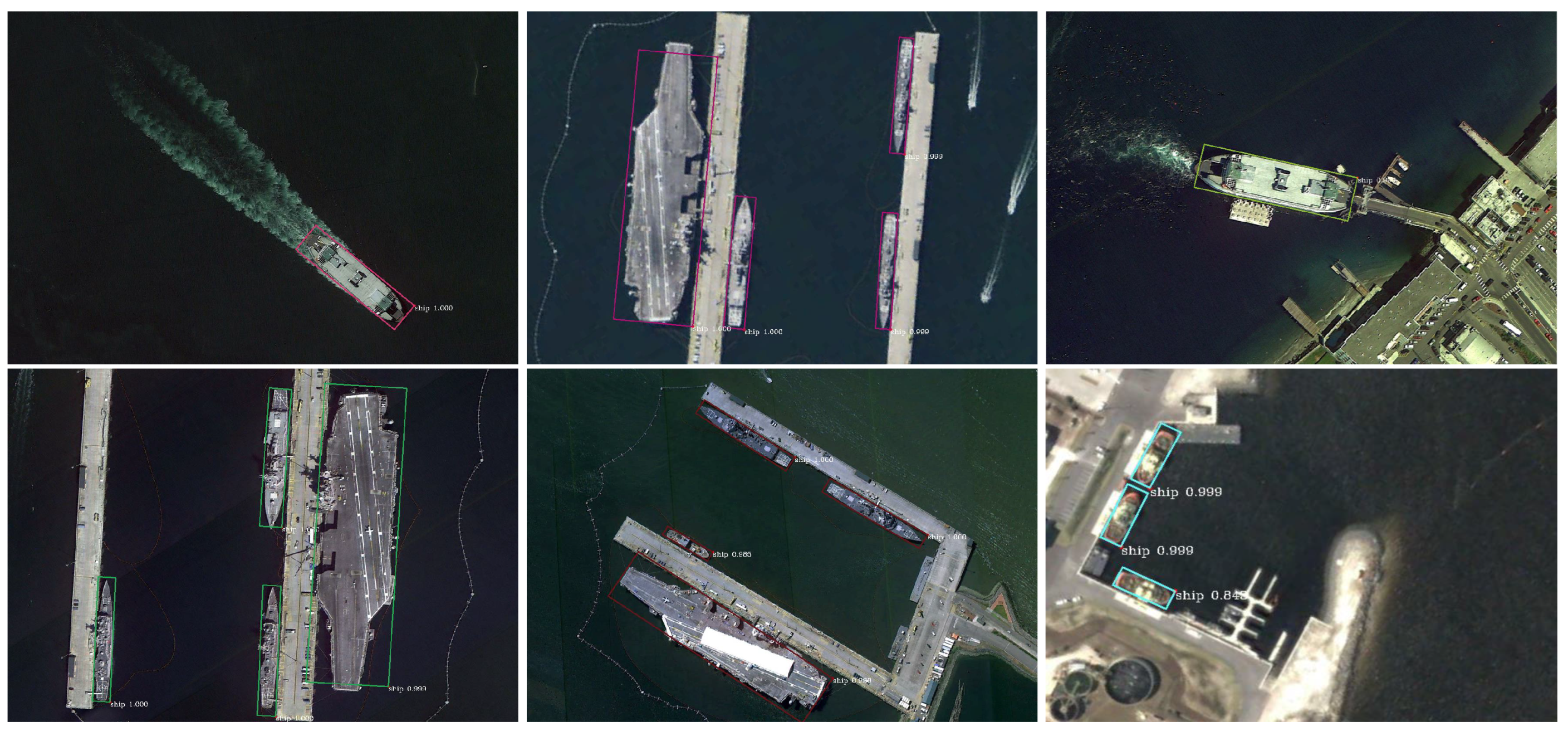
As we can see from Table 3 and Table 5, the improvement of the mAP in our method is at least 0.9 and at most 1.4 on HRSC2016, which is lower than that of at least 1.26 and at most 16.49 on DOTA. Notice that the object in the HRSC2016 dataset belongs to the single category (ship), although the objects have different sizes, aspect ratios, and orientations. Therefore, we suppose that this issue is most likely related to the uniformity of the categories of objects to some extent.

(IV)

Since the main focus of this paper is to explore the potential impact of the variance in the detection error on the performance of detection, we temporarily chose Faster R-CNN as our baseline, which is a classic detector in two-stage detectors. The results show that the scale factor has a significant impact on the detection performance, and the best scale factor is experimentally about 2.0 rather than 1.0, as in the common smooth L${}_1$ loss function. However, we have not yet explored a similar investigation under other baselines adopted in two-stage approaches. Moreover, one might consider similar explorations in one-stage approaches, e.g., YOLO.

5. Conclusions

In this paper, we propose a new two-stage detector for aerial image detection, called Faster R-CNN-NeXt with RoI-Transformer, which is based on the proposed scaled smooth L1 loss function. In our method, by introducing the notion of scale factor, we proposed a new scaled smooth L${}_1$ loss function, which was employed in the bounding box regression. In order to improve the performance, we also paid attention to the issue of searching for the optimal scale factor. Moreover, to deal with the complicated orientations of objects, we incorporated the RoI-Transformer module into our network in order to acquire well-oriented object detection. In addition, we used ResNeXt50(32 × 4) as our backbone instead of ResNet50 as in the standard Faster R-CNN.

To test the effectiveness of the proposed model, we first tested our model with different backbones on DOTA. The overall indicator mAP shows the advantage of ResNeXt. Then, we tested the performance for different values of the scale factor in the scaled smooth L${}_1$ loss function. We tested the effectiveness on two datasets, DOTA and HRSC2016. The results specifically show that the scale factor in the scaled smooth L${}_1$ loss function can affect the performance; the optimal scale factor is about 2.0 for our method, rather than the commonly used 1.0 as in the common smooth L${}_1$ loss function. Regarding DOTA, our method achieves 70.82 mAP with an improvement of at least 1.26 and at most 16.49 compared with FR-O, RPN, R${}^2$CNN, and RoI-Transformer methods. Meanwhile, with HRSC2016, our method achieves 87.1 mAP with an improvement of at least 0.9, and at most 1.4 compared with RC2, R${}^2$PN, RRD, and RoI-Transformer methods.

The values of the scale factor were experimentally set in our study. Further research could focus on developing a self-adaptive way to search for the optimal scale factor. In addition, another interesting and meaningful topic for further study could be to investigate the impact of the scale factor on the detection performance for one-stage detectors, such as YOLO.

References

1. Lim, J.; Astrid, M.; Yoon, H.; Lee, S. Small object detection using context and attention. In Proceedings of the 2021 International Conference on Artificial Intelligence in Information and Communication (ICAIIC), Jeju Island, Republic of Korea, 13–16 April 2021; pp. 181–186. [Google Scholar]
2. EIMikaty, M.; Stathaki, T. Detection of Cars in High-Resolution Aerial images of Complex Urban Environments. IEEE Trans. Geosci. Remote Sens. 2017, 55, 5913–5924. [Google Scholar] [CrossRef]
3. Wang, G.; Wang, X.; Fan, B.; Pan, C. Feature extraction by rotation-invariant matrix representation for object detection in aerial image. IEEE Geosci. Remote Sens. Lett. 2017, 14, 851–855. [Google Scholar] [CrossRef]
4. Cheng, G.; Zhou, P.; Han, J. RIFD-CNN: Rotation-Invariant and Fisher Discriminative Convolutional Neural Networks for Object Detection. In Proceedings of the 2016 IEEE Conference on Computer Vision and Pattern Recognition (CVPR), Seattle, WA, USA, 27–30 June 2016; pp. 2884–2893. [Google Scholar]
5. Deng, Z.; Sun, H.; Zhou, S.; Zhao, J.; Zou, H. Toward fast and accurate vehicle detection in aerial images using coupled region-based convolutional neural networks. J-STARS 2017, 10, 3652–3664. [Google Scholar] [CrossRef]
6. Long, Y.; Gong, Y.; Xiao, Z.; Liu, Q. Accurate Object Localization in Remote Sensing images Based on Convolutional Neural Networks. IEEE Trans. Geosci. Remote Sens. 2017, 55, 2486–2494. [Google Scholar] [CrossRef]
7. Sermanet, P.; Eigen, D.; Zhang, X.; Mathieu, M.; Fergus, R.; Lecun, Y. OverFeat: Integrated recognition, localization and detection using convolutional networks. In Proceedings of the International Conference on Learning Representations, Banff, AB, Canada, 14–26 April 2014. [Google Scholar]
8. Redmon, J.; Divvala, S.; Girshick, R.; Farhadi, A. You Only Look Once: Unified, Real-Time Object Detection. In Proceedings of the 2016 IEEE Conference on Computer Vision and Pattern Recognition (CVPR), Las Vegas, NV, USA, 26 June–1 July 2016; pp. 779–788. [Google Scholar]
9. Redmon, J.; Farhadi, A. YOLO9000: Better, faster, stronger. In Proceedings of the 2017 IEEE Conference on Computer Vision and Pattern Recognition (CVPR), Honolulu, HI, USA, 21–26 July 2017; pp. 517–6525. [Google Scholar]
10. Redmon, J.; Farhadi, A. YOLOv3: An incremental improvement. arXiv 2018, arXiv:1804.02767. [Google Scholar]
11. Bochkovskiy, A.; Wang, C.; Liao, H. YOLOv4: Optimal Speed and Accuracy of Object Detection. arXiv 2020, arXiv:2004.10934. [Google Scholar]
12. Liu, W.; Anguelov, D.; Erhan, D.; Szegedy, C.; Reed, S.; Fu, C.; Berg, A. SSD: Single Shot MultiBox Detector. In Lecture Notes in Computer Science; Springer: Berlin/Heidelberg, Germany, 2016. [Google Scholar]
13. Law, H.; Deng, J. CornerNet: Detecting Objects as Paired Keypoints. In Proceedings of the Computer Vision—ECCV 2018 15th European Conference, Munich, Germany, 8–14 September 2018; Lecture Notes in Computer Science. Springer: Berlin/Heidelberg, Germany, 2018; pp. 765–781. [Google Scholar]
14. Lin, T.; Goyal, P.; Girshick, R.; He, K.; Dollár, P. Focal Loss for Dense Object Detection. IEEE Trans. Pattern Anal. Mach. Intell. 2020, 42, 318–327. [Google Scholar] [CrossRef] [Green Version]
15. Chen, S.; Zhan, R.; Zhang, J. Geospatial Object Detection in Remote Sensing Imagery Based on Multiscale Single-Shot Detector with Activated Semantics. Remote Sens. 2018, 10, 820. [Google Scholar] [CrossRef] [Green Version]
16. Wen, G.; Cao, P.; Wang, H.; Chen, H.; Liu, X.; Xu, J.; Zaiane, Q. MS-SSD: Multi-scale single shot detector for ship detection in remote sensing images. Appl. Intell. 2023, 53, 1586–1604. [Google Scholar] [CrossRef]
17. Etten, A.V. You Only Look Twice: Rapid Multi-Scale Object Detection In Satellite Imagery. arXiv 2018, arXiv:1805.09512. [Google Scholar]
18. Cheng, X.; Zhang, C. C-2-YOLO: Rotating Object Detection Network for Remote Sensing images with Complex Backgrounds. In Proceedings of the 2022 IEEE International Joint Conference on Neural Networks (IJCNN), Padua, Italy, 18–23 July 2022. [Google Scholar]
19. Dong, X.; Qin, Y.; Gao, Y.; Fu, R.; Liu, S.; Ye, Y. Attention-Based Multi-Level Feature Fusion for Object Detection in Remote Sensing images. Remote Sens. 2022, 14, 3735. [Google Scholar] [CrossRef]
20. Lin, T.; Dollar, P.; Girshick, R.; He, K.; Hariharan, B.; Belongie, S. Feature pyramid networks for object detection. In Proceedings of the 2017 IEEE Conference on Computer Vision and Pattern Recognition (CVPR), Honolulu, HI, USA, 21–26 July 2017; pp. 2117–2125. [Google Scholar]
21. Han, J.; Ding, J.; Li, J.; Xia, G. Align Deep Features for Oriented Object Detection. IEEE Trans. Geosci. Remote Sens. 2022, 60, 5602511. [Google Scholar] [CrossRef]
22. Liu, Y.; Li, Q.; Yuan, Y.; Du, Q.; Wang, Q. ABNet: Adaptive Balanced Network for Multiscale Object Detection in Remote Sensing Imagery. IEEE Trans. Geosci. Remote Sens. 2022, 60, 5614914. [Google Scholar] [CrossRef]
23. Liu, Y.; He, G.; Wang, Z.; Li, W.; Huang, H. NRT-YOLO: Improved YOLOv5 Based on Nested Residual Transformer for Tiny Remote Sensing Object Detection. Sensors 2022, 22, 4953. [Google Scholar] [CrossRef] [PubMed]
24. Zakria, Z.; Deng, J.; Kumar, R.; Khokhar, M.; Cai, J.; Kumar, J. Multiscale and Direction Target Detecting in Remote Sensing images via Modified YOLO-v4. IEEE J.-Stars 2022, 15, 1039–1048. [Google Scholar] [CrossRef]
25. Zhou, Q.; Zhang, W.; Li, R.; Wang, J.; Zhen, S.; Niu, F. Improved YOLOv5-S object detection method for optical remote sensing images based on contextual transformer. J. Electron. Imaging 2022, 31, 4. [Google Scholar] [CrossRef]
26. YOLOrs Sharma, M.; Dhanaraj, M.; Karnam, S.; Chachlakis, D.G.; Ptucha, R.; Markopoulos, P.P.; Saber, E. YOLOrs: Object Detection in Multimodal Remote Sensing Imagery. IEEE J. Sel. Top. Appl. Earth Obs. Remote Sens. 2021, 14, 1497–1508. [Google Scholar] [CrossRef]
27. Zhang, J.; Zhang, L.; Liu, T.; Wang, Y. YOLSO: You Only Look Small Object. J. Vis. Commun. Image R. 2021, 81, 103348. [Google Scholar] [CrossRef]
28. Mt-yolov6 Pytorch Object Detection Model. Available online: https://models.roboflow.com/object-detection/mt-yolov6 (accessed on 23 June 2022).
29. Yolov7 Pytorch Object Detection Model. Available online: https://models.roboflow.com/object-detection/yolov7 (accessed on 6 July 2022).
30. Uijlings, J.R.R.; van de Sande, K.E.A.; Gevers, T.; Smeulders, A.W.M. Selective search for object recognition. Int. J. Comput. Vis. (IJCV) 2013, 104, 154–171. [Google Scholar] [CrossRef] [Green Version]
31. Girshick, R.; Donahue, J.; Darrell, T.; Malik, J. Rich feature hierarchies for accurate object detection and semantic segmentation. In Proceedings of the 2014 IEEE Conference on Computer Vision and Pattern Recognition (CVPR), Columbus, OH, USA, 23–28 June 2014; pp. 580–587. [Google Scholar]
32. Girshick, R. Fast R-CNN. In Proceedings of the 2015 IEEE Conference on Computer Vision and Pattern Recognition (CVPR), Santiago, Chile, 11–18 December 2015; pp. 1440–1448. [Google Scholar]
33. Ren, S.; He, K.; Girshick, R.; Sun, J. Faster R-CNN: Towards Real-Time Object Detection with Region Proposal Networks. IEEE Trans. Pattern Anal. Mach. Intell. 2017, 39, 1137–1149. [Google Scholar] [CrossRef] [Green Version]
34. Li, Z.; Wang, Y.; Zhang, N.; Zhang, Y.; Zhao, Z.; Xu, D.; Ben, G.; Gao, Y. Deep Learning-Based Object Detection Techniques for Remote Sensing images: A Survey. Remote Sens. 2022, 14, 2385. [Google Scholar] [CrossRef]
35. Cheng, G.; Zhou, P.; Han, J. Learning rotation-invariant convolution neural networks for object detection in VHR optical remote sensing images. IEEE Trans. Geosci. Remote Sens. 2016, 54, 7405–7415. [Google Scholar] [CrossRef]
36. Neubeck, A.; Van Gool, L. Efficient non-maximum suppression. In Proceedings of the 2006 International Conference on Pattern Recognition (ICPR06), Hong Kong, China, 20–24 August 2006; pp. 850–855. [Google Scholar]
37. Liu, Z.; Wang, H.; Weng, L.; Yang, Y. Ship rotated bounding box space for ship extraction from high-resolution optical satellite images with complex backgrounds. IEEE Geosci. Remote Sens. Lett. 2016, 13, 1074–1078. [Google Scholar] [CrossRef]
38. Xia, G.; Bai, X.; Ding, J.; Zhu, Z.; Belongie, S.; Luo, J.; Datcu, M.; Pelillo, M.; Zhang, L. Dota: A large-scale dataset for object detection in aerial images. In Proceedings of the 2018 IEEE Conference on Computer Vision and Pattern Recognition, Salt Lake City, UT, USA, 18–23 June 2018; pp. 3974–3983. [Google Scholar]
39. Liu, K.; Mattyus, K. Fast multiclass vehicle detection on aerial images. IEEE Geosci. Remote Sens. Lett. 2015, 12, 1938–1942. [Google Scholar]
40. Ma, J.; Shao, W.; Ye, H.; Wang, L.; Wang, H.; Zheng, Y.; Xue, X. Arbitrary-oriented scene text detection via rotation proposals. IEEE Trans. Multimed. 2018, 20, 3111–3122. [Google Scholar] [CrossRef] [Green Version]
41. Zhang, Z.; Guo, W.; Zhu, S.; Yu, W. Toward arbitrary-oriented ship detection with rotated region proposal and discrimination networks. IEEE Geosci. Remote Sens. Lett. 2018, 99, 1745–1749. [Google Scholar] [CrossRef]
42. Yang, X.; Sun, H.; Fu, K.; Yang, J.; Sun, X.; Yan, M.; Guo, Z. Automatic ship detection in remote sensing images from google earth of complex scenes based on multiscale rotation dense feature pyramid networks. Remote Sens. 2018, 10, 132. [Google Scholar] [CrossRef] [Green Version]
43. Azimi, S.; Vig, E.; Bahmanyar, R.; Korner, M.; Reinartz, P. Towards multi-class object detection in unconstrained remote sensing imagery. arXiv 2018, arXiv:1807.02700. [Google Scholar]
44. Yu, D.; Ji, S. A New Spatial-Oriented Object Detection Framework for Remote Sensing images. IEEE Trans. Geosci. Remote Sens. 2022, 60, 4407416. [Google Scholar] [CrossRef]
45. Ma, T.; Mao, M.; Zheng, H.; Gao, P.; Wang, X.; Han, S.; Ding, E.; Zhang, B.; Doermann, D. Oriented object detection with transformer. arXiv 2021, arXiv:2106.03146. [Google Scholar]
46. Liu, L.; Pan, Z.; Lei, B. Learning a rotation invariant detector with rotatable bounding box. arXiv 2017, arXiv:1711.09405. [Google Scholar]
47. Liu, Z.; Hu, J.; Weng, L.; Yang, Y. Rotated region based cnn for ship detection. In Proceedings of the 2017 IEEE International Conference on Image Processing (ICIP), Beijing, China, 17–20 September 2017; pp. 900–904. [Google Scholar]
48. Yang, X.; Yan, J. Arbitrary-oriented object detection with circular smooth label. In Proceedings of the Computer Vision—ECCV 2020: 16th European Conference, Glasgow, UK, 23–28 August 2020; pp. 677–694. [Google Scholar]
49. Xu, Y.; Fu, M.; Wang, Q.; Wang, Y.; Chen, K.; Xia, G.; Bai, X. Gliding vertex on the horizontal bounding box for multi-oriented object detection. IEEE Trans. Pattern Anal. Mach. Intell. 2020, 43, 1452–1459. [Google Scholar] [CrossRef] [PubMed] [Green Version]
50. Huang, Z.; Li, W.; Xia, X.; Wang, H.; Jie, F.; Tao, R. LO-Det: Lightweight Oriented Object Detection in Remote Sensing images. IEEE Trans. Geosci. Remote Sens. 2022, 60, 223373–223384. [Google Scholar] [CrossRef]
51. Ding, J.; Xue, N.; Long, Y.; Xia, G.; Lu, Q. Learning roi transformer for oriented object detection in aerial images. In Proceedings of the 2019 IEEE Conference on Computer Vision and Pattern Recognition (CVPR), Long Beach, CA, USA, 16–20 June 2019; pp. 2844–2853. [Google Scholar]
52. Li, Z.; Peng, C.; Yu, G.; Zhang, X.; Deng, Y.; Sun, J. Light-Head R-CNN: In defense of two-stage object detector. arXiv 2017, arXiv:1711.07264. [Google Scholar]
53. He, K.; Zhang, X.; Ren, S.; Sun, J. Deep residual learning for image recognition. In Proceedings of the 2016 IEEE Conference on Computer Vision and Pattern Recognition (CVPR), Seattle, WA, USA, 27–30 June 2016; pp. 770–778. [Google Scholar]
54. Yang, X.; Yang, J.; Yan, J.; Zhang, Y.; Zhang, T.; Guo, Z.; Sun, X.; Fu, K. Scrdet: Towards more robust detection for small, cluttered and rotated objects. In Proceedings of the 2019 IEEE/CVF International Conference on Computer Vision (ICCV), Seoul, Republic of Korea, 27 October–2 November 2019; pp. 8231–8240. [Google Scholar]
55. Hastie, T.; Tibshirani, R.; Friedman, J. The Elements of Statistical Learning; Springer: Berlin/Heidelberg, Germany, 2008. [Google Scholar]
56. Xie, S.; Girshick, R.; He, K. Aggregated residual transformations for deep neural networks. In Proceedings of the 2017 IEEE Conference on Computer Vision and Pattern Recognition (CVPR), Honolulu, HI, USA, 21–26 July 2017; pp. 5987–5995. [Google Scholar]
57. Dai, J.; Li, Y.; He, K.; Sun, J. R-FCN: Object Detection via Region-based Fully Convolutional Networks. In Proceedings of the 2016 Conference on Neural Information Processing Systems (NIPS), Barcelona, Spain, 5–10 December 2016. [Google Scholar]
58. Cai, Z.; Vasconcelos, N. Cascade r-cnn: Delving into high quality object detection. In Proceedings of the 2018 IEEE Conference on Computer Vision and Pattern Recognition (CVPR), Salt Lake City, UT, USA, 18–23 June 2018; pp. 6154–6162. [Google Scholar]
59. Li, J.; Tian, Y.; Xu, Y.; Hu, X.; Zhang, Z.; Wang, H.; Xiao, Y. MM-RCNN: Toward Few-Shot Object Detection in Remote Sensing images with Meta Memory. IEEE Trans. Geosci. Remote Sens. 2022, 60, 5635114. [Google Scholar] [CrossRef]
60. Shivappriya, S.; Priyadarsini, M.; Stateczny, A.; Puttamadappa, C.; Parameshachari, B. Cascade Object Detection and Remote Sensing Object Detection Method Based on Trainable Activation Function. Remote Sens. 2021, 13, 200. [Google Scholar] [CrossRef]
61. Samanta, S.; Panda, M.; Ramasubbareddy, S.; Sankar, S.; Burgos, D. Spatial-Resolution Independent Object Detection Framework for Aerial Imagery. CMC Comput. Mater. Contin. 2021, 68, 1937–1948. [Google Scholar] [CrossRef]
62. Liu, R.; Yu, Z.; Mo, D.; Cai, Y. An Improved Faster-RCNN Algorithm for Object Detection in Remote Sensing images. In Proceedings of the Chinese Control Conference (CCC), Shenyang, China, 27–29 July 2020; pp. 7188–7192. [Google Scholar]
63. Zhang, Y.; Song, C.; Zhang, D. Small-scale aircraft detection in remote sensing images based on Faster-RCNN. Multimed. Tools Appl. 2022, 81, 13. [Google Scholar] [CrossRef]
64. Luo, M.; Tian, Y.; Zhang, S.; Huang, L.; Wang, H.; Liu, Z.; Yang, L. Individual Tree Detection in Coal Mine Afforestation Area Based on Improved Faster RCNN in UAV RGB images. Remote Sens. 2022, 14, 5545. [Google Scholar] [CrossRef]
65. Szegedy, C.; Liu, W.; Jia, Y.; Sermanet, P.; Reed, S.; Anguelov, D.; Erhan, D.; Vanhoucke, V.; Rabinovich, A. Going deeper with convolutions. In Proceedings of the 2015 IEEE Conference on Computer Vision and Pattern Recognition (CVPR), Boston, MA, USA, 7–12 June 2015; pp. 1–9. [Google Scholar]
66. Szegedy, C.; Vanhoucke, V.; Ioffe, S.; Shlens, J.; Wojna, Z. Rethinking the inception architecture for computer vision. In Proceedings of the 2016 IEEE Conference on Computer Vision and Pattern Recognition(CVPR), Seattle, WA, USA, 27–30 June 2016; pp. 2818–2826. [Google Scholar]
67. Liu, Z.; Yuan, L.; Weng, L.; Yang, Y. A High Resolution Optical Satellite Image Dataset for Ship Recognition and Some New Baselines. In Proceedings of the 2017 International Conference on Pattern Recognition Applications and Methods (ICPRAM), Porto, Portugal, 24–26 February 2017; pp. 324–331. [Google Scholar]
68. Schmidt, M.; Le Roux, N.; Bach, F. Minimizing finite sums with the stochastic average gradient. Math. Program. 2017, 162, 83–112. [Google Scholar] [CrossRef] [Green Version]
69. Ioffe, S.; Szegedy, C. Batch normalization: Accelerating deep network training by reducing internal covariate shift. In Proceedings of the 2015 International Conference on Machine Learning, Lille, France, 7–9 July 2015; pp. 448–456. [Google Scholar]
70. Deng, J.; Dong, W.; Socher, R.; Li, L.; Li, K.; Li, F. ImageNet:A large-scale hierarchical image database. In Proceedings of the 2009 IEEE Conference on Computer Vision and Pattern Recognition (CVPR), Miami, FL, USA, 20–25 June 2009; pp. 248–255. [Google Scholar]
71. Jiang, Y.; Zhu, X.; Wang, X.; Yang, X.; Li, W.; Wang, H.; Fu, P.; Luo, Z. R2cnn: Rotational region cnn for robust scene text detection. arXiv 2017, arXiv:1706.09579. [Google Scholar]
72. Liao, M.; Zhu, Z.; Shi, B.; Xia, G.; Bai, X. Rotation-sensitive regression for oriented scene text detection. In Proceedings of the 2018 IEEE Conference on Computer Vision and Pattern Recognition (CVPR), Salt Lake City, UT, USA, 18–23 June 2018; pp. 5909–5918. [Google Scholar]
Figure 1. Instances from a bird’s-eye view. The images are from the DOTA dataset. There are challenges and difficulties in detecting remote sensing images. (a) Small and densely packed objects. (b) Objects with complicated backgrounds. (c) Objects with arbitrary orientation.
Remotesensing 15 01350 g001
Figure 2. Horizontal bounding boxes versus oriented bounding boxes.
Remotesensing 15 01350 g002
Figure 3. Visualization of the detection error.
Remotesensing 15 01350 g003
Figure 4. Architecture of Faster R-CNN-NeXt with RoI-Transformer.
Remotesensing 15 01350 g004
Figure 5. (Left) a unit of ResNet. (Right) a unit of ResNeXt.
Remotesensing 15 01350 g005
Figure 6. The schematic map of complexity on channels. (a) stands for ResNet. (b) stands for ResNeXt (4 × 2). (c) stands for ResNeXt (2 × 4). The green circles represent the input features whose number represents the number of channels about features. The yellow circles represent the output features. The purple circles represent the middle features.
Remotesensing 15 01350 g006
Figure 7. The architecture of combining ResNeXt and FPN. The CT denotes the channel transformer with Conv 1 × 1, which converts different layers with different channel numbers into layers with the same number of channels. The MP stands for max pooling. Moreover, 2× up means upsampling by a multiple of 2.
Remotesensing 15 01350 g007
Figure 8. The structure of the RoI-Transformer. The input features (i.e., green cubes) with the HRoI (i.e., the area features of black bounding box) pass into RoI-Transformer to obtain RRoIs (i.e., the red cube). The RoI-Transformer consists of two parts, RRoI learner and RoI Align, where the RRoI learner is completed through the fully connected layer to learn the 5 parameters of the RGT (i.e., rotated ground truth) relative to HRoIs.
Remotesensing 15 01350 g008
Figure 9. Change from HBB regression (a) to RBB regression (b).
Remotesensing 15 01350 g009
Figure 10. Training losses with iterations, where loc and cls losses represent the regression loss (i.e., location loss) and the classification loss respectively. (a) Training losses in the RPN stage. (b) Training losses in the RoI-Transformer stage. (c) Training losses in the final predict stage. (d) The overall total loss in training.
Remotesensing 15 01350 g010
Figure 11. Visualization of results on the DOTA test dataset.
Remotesensing 15 01350 g011
Figure 12. Visualization of the results under different scale factors.
Remotesensing 15 01350 g012
Figure 13. Visualization of results on the HRSC2016 test dataset.
Remotesensing 15 01350 g013